Estimation of the Equivalent Circuit Parameters in Transformers Using Evolutionary Algorithms

Abstract

The conventional methods of parameter estimation in transformers, such as the open-circuit and short-circuit tests, are not always available, especially when the transformer is already in operation and its disconnection is impossible. Therefore, alternative (non-interruptive) methods of parameter estimation have become of great importance. In this work, no-interruption, transformer equivalent circuit parameter estimation is presented using the following metaheuristic optimization methods: the genetic algorithm (GA), particle swarm optimization (PSO) and the gravitational search algorithm (GSA). These algorithms provide a maximum average error of 12%, which is twice as better as results found in the literature for estimation of the equivalent circuit parameters in transformers at a frequency of 50 Hz. This demonstrates that the proposed GA, PSO and GSA metaheuristic optimization methods can be applied to estimate the equivalent circuit parameters of single-phase distribution and power transformers with a reasonable degree of accuracy.

1. Introduction

A transformer is an essential part of an electric power system, which makes it the objective of a great number of studies focused on obtaining the most complete information about its performance. Single-phase transformer equivalent circuit parameters (SPTECPs) provide necessary information of transformer performance under different operating conditions. Recently, some research works have focused on obtaining SPTECPs. Some of them used different computational algorithms, black box models and transfer function methods [1,2]. The least squares method has also been used to estimate the equivalent circuit parameters of an n-winding transformer in operation [3]. Within this methodology, in [3], SPTECPs were obtained in two steps: first, the parameters of windings and then those of the core were obtained. Another method of SPTECP estimation in real time consists of measuring voltages and currents on windings and using the LabVIEW platform for collecting and processing data. In [2], the results calculated via LabVIEW were compared with those obtained in the open-circuit and short-circuit tests. The GA and PSO metaheuristic algorithms for the estimation of SPTECPs were not very efficient and were inaccurate in the work of [4] compared to the conventional open-circuit and short-circuit tests, which showed a maximum average error of 24%. In turn, the GSA and imperialist competitive algorithms (ICA) were more accurate in [5]. The bacterial foraging algorithm (BFA) for SPTECP estimation uses the objective function, which depends on voltage and active power. In [6], the estimates were compared with the results of the load, voltage regulation and efficiency tests. The chaotic optimization approach (COA) is another method for SPTECP estimation. The comparison of the COA with the results of the GA, PSO, the GSA, the ICA and the BFA can be found in [4,5,6]. In [7], a variety of objective functions within the COA method was used.

However, single-phase power transformers have not been the focus of the aforementioned works, and the respective optimization methods and algorithms have not yet been tested on this class of power transformers. At the same time, SPTECP values are not always available for modeling and simulating single-phase power transformers, which makes the analysis of their performance under different operating conditions difficult, especially for failure prevention. This is why SPTECP estimation of single-phase power transformers is of great importance. In this paper, the GA, PSO and the GSA optimization methods are effectively applied to a single-phase power transformer of a 4 kVA up to 33 MVA capacity with 50 and 60 Hz of frequencies for the estimation of SPTECPs. These were chosen as representative approaches of evolutionary algorithms (the GA), swarm intelligence (PSO) and physics-based algorithms (the GSA). The implementation of these optimization technics prevent the necessity of a power system interruption once the transformer has been installed and put in operation.The advantage of using metaheuristic optimization methods, such as the GA, PSO and the GSA, to estimate SPTECPs is that they only require knowledge of the rated capacity of the transformer and the voltages and currents measured in its primary and secondary windings, given that the transformer is operating at full load (unitary power factor). This allows one to evaluate SPTECPs without having to refer to the equipment manual (e.g., if it is not available) and without stopping the equipment. In addition, our algorithms show a higher accuracy for the analyzed case studies. The reader can consult the corresponding computer programs of this research by referring to the following Computer programs (accessed on 24 January 2023). The use of the free Python 3.9 software library was allowed in order to avoid additional expenses.

The organization of this paper is as follows: Section 2 describes the parameters of the single-phase transformer equivalent circuit and objective function; Section 3 presents the metaheuristic optimization methods used to solve our case of study; briefly, we explain the simulation and results that we obtained for our three case studies of the single-phase transformer in Section 4; in Section 5 our conclusions and future work are presented.

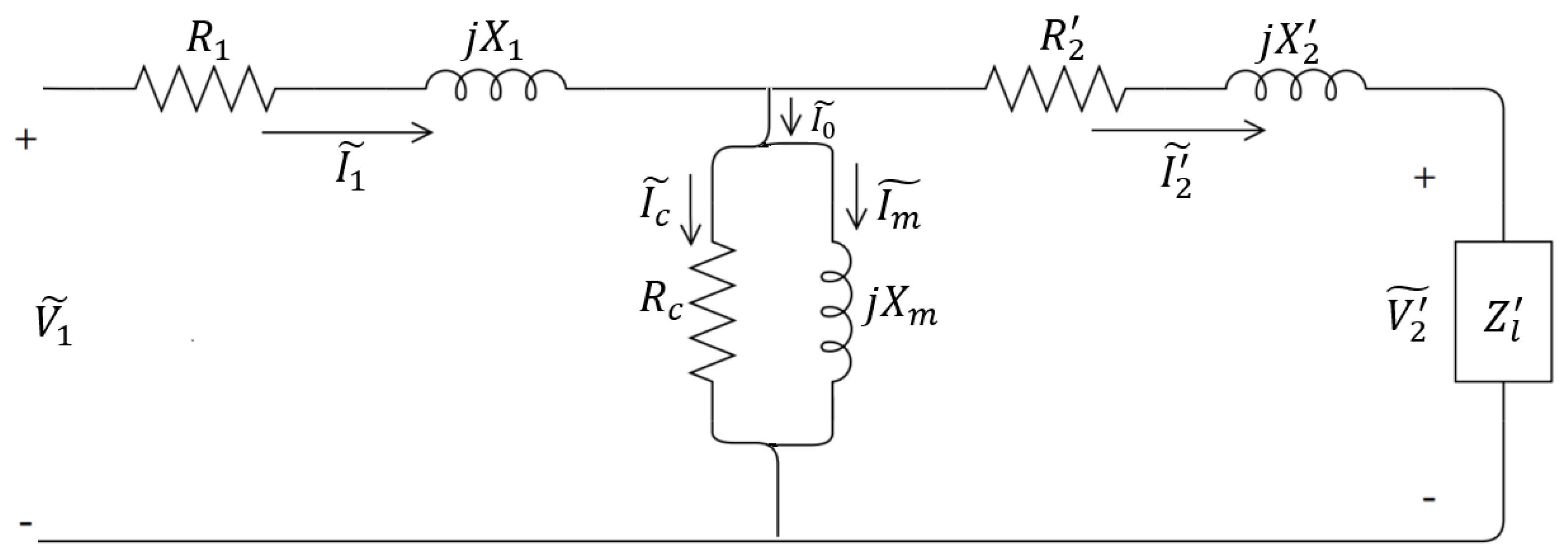
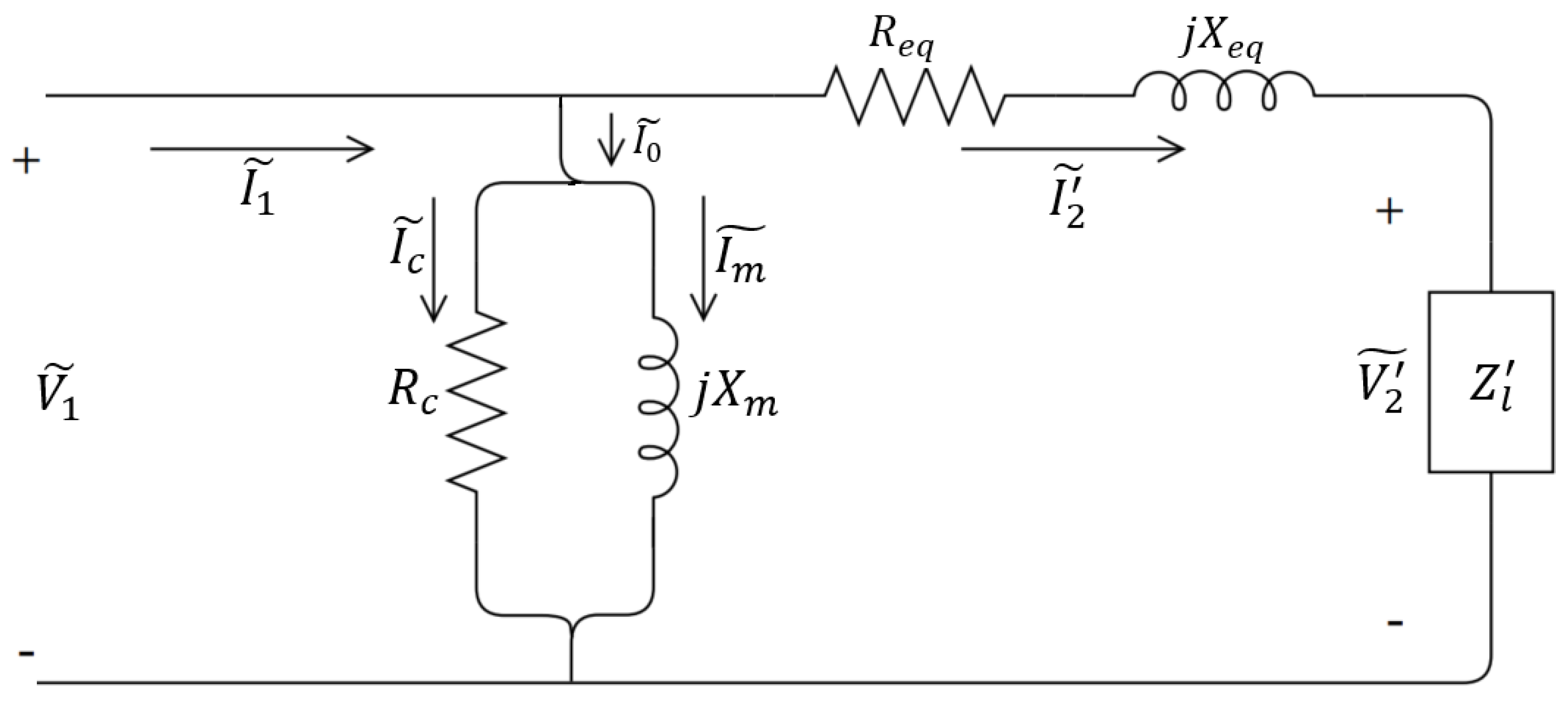
2. The Single-Phase Transformer Equivalent Circuit

An equivalent circuit is a powerful tool in electrical engineering that retains all of the electrical characteristics of a given electric system. Figure 1 shows the equivalent circuit of the single-phase transformer with respect to the primary winding, where we have the following.

$R_1$: primary winding resistance;

$j{X}_1$: primary winding reactance;

$R_2^{\prime }$: secondary winding resistance with respect to the primary side;

$j{X}_2^{\prime }$: secondary leakage reactance with respect to the primary side;

$R_c$: core resistance;

$j{X}_m$: magnetizing reactance.

To calculate the RMS alternating current and voltage, the grid equations are derived from Kirchhoff’s law of voltages,

$$\begin{array}{c}\hfill -\widetilde{V_1}+Z_1\widetilde{I_1}+Z_0(\widetilde{I_1}-\widetilde{I_2^{\prime }})=0\end{array}$$

(1)

$$\begin{array}{c}\hfill Z_2\widetilde{I_2^{\prime }}+Z_l^{\prime }\widetilde{I_2^{\prime }}+Z_0(\widetilde{I_2^{\prime }}-\widetilde{I_1})=0\end{array}$$

(2)

where the impedances are as follows:

$$\begin{array}{c}\hfill Z_1=R_1+j{X}_1,Z_2=R_2^{\prime }+j{X}_2^{\prime }\mathrm{and}{Z}_0=\frac{j{R}_c{X}_m}{R_c+j{X}_m}.\end{array}$$

Solving the system of equations we obtain $I_{1est}$, $I_{2est}^{{}^{\prime }}$ and $V_{2est}^{{}^{\prime }}$, which are the estimated RMS values to be substituted into the objective function

$$\begin{array}{c}\hfill \widetilde{I_1}=\frac{\widetilde{V_1}(Z_0+Z_2+Z_l^{\prime })}{▵}\end{array}$$

(3)

$$\begin{array}{c}\hfill \widetilde{I_2^{\prime }}=\frac{\widetilde{V_1}{Z}_0}{▵}\end{array}$$

(4)

$$\begin{array}{c}\hfill \widetilde{V_2^{\prime }}=\widetilde{I_2^{\prime }}{Z}_l^{\prime }\end{array}$$

(5)

where,

$$\begin{array}{c}\hfill ▵=\left((Z_1+Z_0)(Z_0+Z_2+Z_l^{\prime })\right)-Z_0^2.\end{array}$$

Therefore,

$$\begin{array}{c}\hfill I_{1est}=|\widetilde{I_1}|I_{2est}^{{}^{\prime }}=|\widetilde{I_2^{{}^{\prime }}}|\mathrm{and}{V}_{2est}^{{}^{\prime }}=\left|\widetilde{V_2^{{}^{\prime }}}\right|.\end{array}$$

In the case of the core losses represented by $R_c$ which are minimal, we use the approximate equivalent circuit of the transformer shown in Figure 2 to obtain the losses and efficiency. The winding losses can be obtained from

$$\begin{array}{c}\hfill P_{cu}=R_{eq}{\left(I_{2est}^{{}^{\prime }}\right)}^2,\end{array}$$

(6)

where

$$\begin{array}{c}\hfill R_{eq}=R_1+R_2^{{}^{\prime }}and{X}_{eq}=X_1+X_2^{{}^{\prime }};\end{array}$$

and the core losses can be obtained from

$$\begin{array}{c}\hfill P_n=\frac{|\widetilde{V_1^2}|}{R_c},\end{array}$$

(7)

where

$$\begin{array}{c}\hfill \widetilde{V_1}=\widetilde{V_2^{{}^{\prime }}}+R_{eq}\widetilde{I_2^{{}^{\prime }}}+X_{eq}\widetilde{I_2^{{}^{\prime }}}\end{array}$$

(8)

and the power out is given by

$$\begin{array}{c}\hfill P_{out}=Z_l^{{}^{\prime }}{\left(I_{2est}^{{}^{\prime }}\right)}^2,\end{array}$$

(9)

the power input is given by

$$\begin{array}{c}\hfill P_{in}=P_{out}+P_{cu}+P_n,\end{array}$$

(10)

and the efficiency is given by

$$\begin{array}{c}\hfill \eta =\frac{P_{out}}{P_{int}}\times 100.\end{array}$$

(11)

The objective function for SPTECP estimation is the following sum of squared errors:

$$\begin{array}{c}\hfill OF=min\left\{{(I_1-I_{1est})}^2+{(I_2^{\prime }-I_{2est}^{\prime })}^2+{(V_2^{\prime }-V_{2est}^{\prime })}^2\right\}\end{array}$$

(12)

where $I_1$, $I_2^{\prime }$ are the measured RMS values of the primary and secondary currents, respectively, with respect to the primary side; $V_2^{\prime }$ is the measured RMS value of the secondary voltage with respect to the primary side of the single-phase transformer; $I_{1est}$, $I_{2est}^{\prime }$ are the estimated values of the primary and secondary currents, respectively, with respect to the primary side; and $V_{2est}^{\prime }$ is the estimated value of the secondary voltage with respect to the primary side obtained from optimization.

3. Optimization Algorithms

3.1. The Genetic Algorithm

The genetic Algorithm is a metaheuristic method proposed by John H. Holland in the early 1960s based on the “survival of the fittest” [8]. This method consists of creating a random initial population of $NP$ individuals with dimension of D elements (we used a real-coded GA). In the case of SPTECP estimation, the individuum X is composed of six elements, $R_1$, $X_1$, $R_2^{\prime }$, $X_2^{\prime }$, $R_c$ and $X_m$, and is a potential solution of the SPTECP. The fitness of each X is calculated using (12) so that the individuals with the best fitness are selected and the worst are rejected. The best individuals, known as parents, are mated with a certain probability, generating, thereby, a new population. Subsequently, the new individuals (known as children) mutate with respective probabilities and they are then submitted to a selection procedure, which consists of keeping the best individual X at each generation (elitism). Thus, a new population with better characteristics is created to guarantee optimal convergence. This procedure is repeated until a certain number of generations $NG$ is reached or any other stopping criterion is accomplished.

Algorithm 1 shows the steps to be followed in order to find the solution for the equivalent circuit parameters of a single-phase transformer.

Algorithm 1: GA

Require:$I_1,$$I_2^{\prime }$ and $V_2^{\prime }$; 1: for i = 1 to NP do 2:    Create $X_i=[R_1,X_1,R_2^{\prime },X_2^{\prime },R_c,X_m]$; 3: end for 4: for i = 1 to NP do 5:     Evaluate (12); 6: end for 7: for gen = 1 to NG do 8:       Select NP individuals based on fitness from X; 9:       Apply crossover operator to individuals selected to generate NP children; 10:     Apply mutation operator to the NP children; 11:     Keep the NP children and discard the NP individuals in X, just keeping the best solution to replace the worst child; 12: end for Ensure: $X_{sol}=[R_1,X_1,R_2^{\prime },X_2^{\prime },R_c,X_m]$.

3.2. Particle Swarm Optimization

The particle swarm optimization algorithm was proposed by Kennedy and Eberhart in 1995 and emulates the social behavior of birds [9]. Swarm members communicate as a group when moving or hunting. The method consists of creating a certain number $NP$ of particles placed in the domain of the objective function (12) where the solution is to be sought. Each particle is a potential solution to the problem. Particles move, remembering their best solution so far ($pbest$) and are able to identify the best solution in the swarm ($gbest$). At each iteration, the position and velocity are updated according to the following equations:

$$\begin{array}{c}\hfill v_{i,j}^g=K(v_{i,j}^{g-1}+C_1{r}_1(pbes{t}_{i,j}^{g-1}-Particl{e}_{i,j}^{g-1})+C_2{r}_2(gbes{t}_{i,j}^{g-1}-Particl{e}_{i,j}^{g-1})),\end{array}$$

(13)

$$Particl{e}_{i,j}^g=Particl{e}_{i,j}^{g-1}+v_{i,j}^g.$$

(14)

Equation (13), which is known as constriction factor PSO [10] is composed of three elements: the first is the previous velocity value, the second is the linear attraction towards the best position recorded by the particle so far ($pbest$) and the third is the linear attraction towards the best global position ($gbest$). The values $C_1$ and $C_2$ are positive constants that control the influence of $gbest$ and $pbest$, respectively: the closer the constants are to zero, the narrower the search, whereas the closer the constants are to one another, the broader the search [11]. Equation (14) is used to update the position of particles. The PSO algorithm is described in Algorithm 2.

Algorithm 2: PSO

Require:$I_1,$$I_2^{\prime }$ and $V_2^{\prime }$; 1: for i = 1 to NP do 2:     Create $Particl{e}_i=[R_1,X_1,R_2^{\prime },X_2^{\prime },R_c,X_m]$; 3: end for 4: for i = 1 to NP do 5:     Evaluate (12); 6: end for 7: while g < NGs do 8:     for i = 1 to NP do 9:         for j = 1 to D = (6) do 10:            $r_1$, $r_2$ = $rand[0,1]$; 11:            Update velocity (13); 12:            Update position (14); 13:         end for 14:         if $f\left(Particl{e}_i^g\right)\le f\left(pbes{t}_i^{g-1}\right)$ then 15:            $pbes{t}_i^g=Particl{e}_i^g$; 16:         end if 17:     end for 18:     if $f\left(Particl{e}_i^g\right)\le f\left(gbes{t}_i^{g-1}\right)$ then 19:         $gbes{t}_i^g=Particl{e}_i^g$; 20:     end if 21: end while Ensure: $Particl{e}_{sol}=[R_1,X_1,R_2^{\prime },X_2^{\prime },R_c,X_m]$.

3.3. The Gravitational Search Algorithm

The gravitational search algorithm is based on the gravitational interaction between masses [12]. The algorithm consists of masses that are attracted to each other, and the lighter weight moves towards the heavier due to the gravitational force [13]. This optimization procedure creates $NP$ random masses that are potential solutions, i.e., the parameters of the transformer, which are evaluated with the objective function (12). The gravitational constant G is calculated starting from an initial point, reducing at each iteration. The values $best$ and $worst$ are obtained from the evaluation of (12), assuming that the inertial, gravitational active and gravitational passive masses are equal and the inertial mass is normalized. The gravitational force $F_{ij}$ is directed from mass i to mass j. In order to obtain the total force acting on a mass, it is necessary to use a function known as $kbest$ that starts at the total number of masses and decreases to one. Therefore, the acceleration of each mass is calculated by updating the velocity and position of the mass until the maximum number $NG$ of iterations is reached. The GSA algorithm is described in Algorithm 3.

Algorithm 3: GSA

Require:$I_1,$$I_2^{\prime }$ and $V_2^{\prime }$; 1: for i = 1 to NP do 2:     Create $mas{s}_i=[R_1,X_1,R_2^{\prime },X_2^{\prime },R_c,X_m]$; 3: end for 4: for i = 1 to NP do 5:     Evaluate (12); 6: end for 7: for t = 1 to NGs do 8:       $G\left(t\right)=Goexp\left(-\alpha \frac{t}{NGs}\right)$; 9:       $best\left(t\right)=mi{n}_{j\in [1,\dots ,NP]}fi{t}_j\left(t\right)$; 10:     $worst\left(t\right)=ma{x}_{j\in [1,\dots ,NP]}fi{t}_j\left(t\right)$; 11:     $M_i=M_{ii}=M_{ai}=M_{pi}$; 12:     $m_i\left(t\right)=\frac{fi{t}_i\left(t\right)-worst\left(t\right)}{best\left(t\right)-worst\left(t\right)}$; 13:     $M_i=\frac{m_i\left(t\right)}{{\sum }_{j=1}^{NP}{m}_j\left(t\right)}$; 14:     for i = 1 to NP do 15:         for j = 1 to Kbest do 16:            if $i\ne j$ then 17:                $F_{ij}\left(t\right)=G\left(t\right)\frac{M_i\left(t\right)}{Rij{\left(t\right)}^R+ϵ}(mas{s}_j\left(t\right)-mas{s}_i\left(t\right))$; 18:            end if 19:         end for 20:     end for 21:     for i = 1 to NP do 22:         for j = 1 to d = 6 do 23:            $a_i^d=\frac{F_i^d}{Mii\left(t\right)}$; 24:            $v_i^d(t+1)=rand[0,1]v_i^d\left(t\right)+a_i^d$; 25:            $mas{s}_i^d(t+1)=mas{s}_i^d\left(t\right)+v_i^d(t+1)$; 26:         end for 27:     end for 28: end for Ensure: $mas{s}_{sol}=[R_1,X_1,R_2^{\prime },X_2^{\prime },R_c,X_m]$.

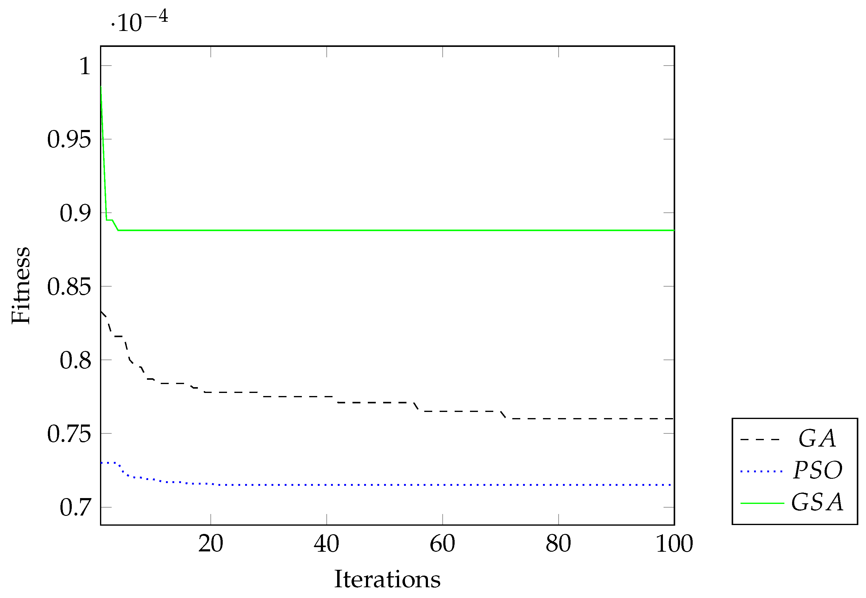
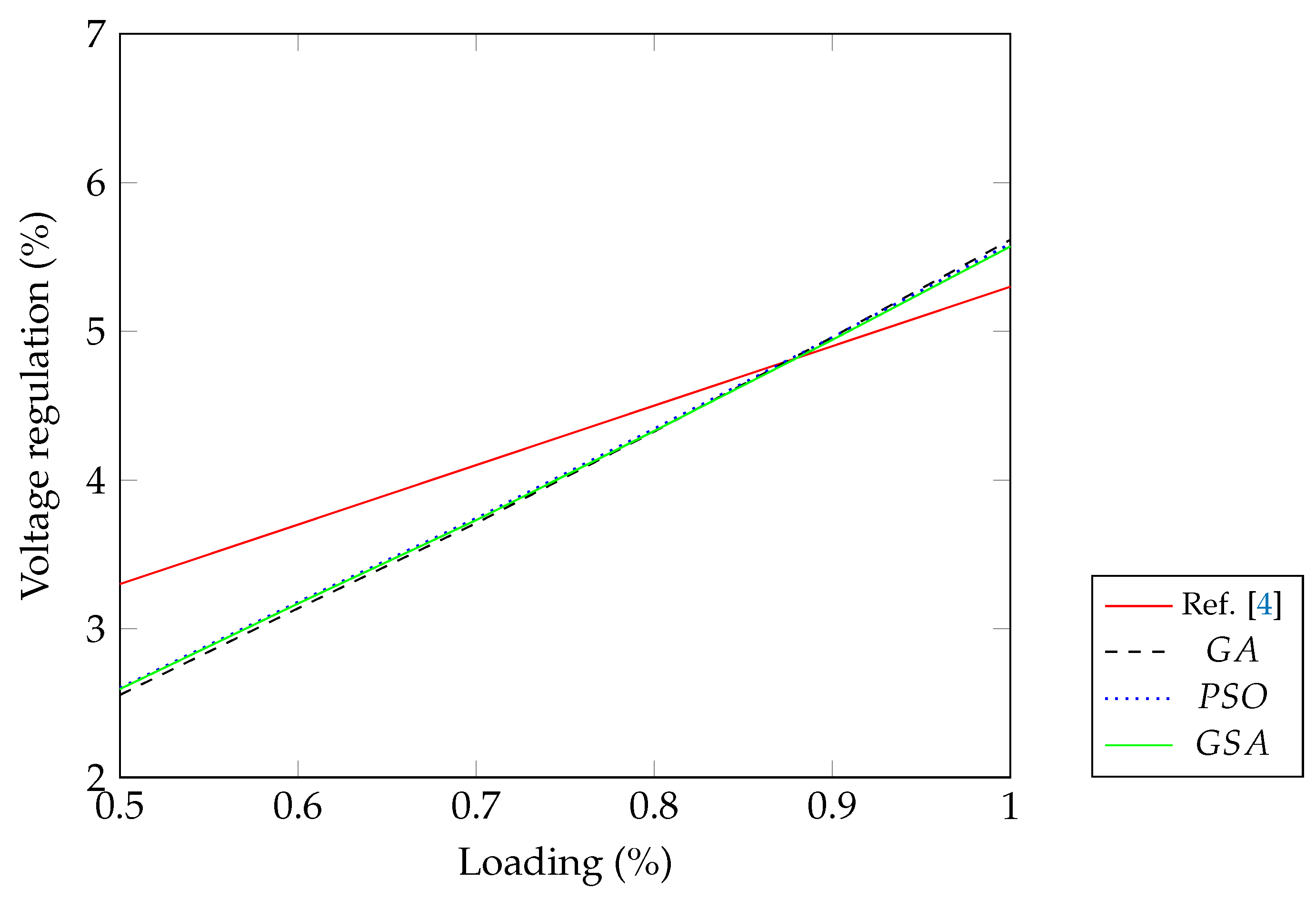
4. Simulation and Results

In order to assess the performance of the above-mentioned optimization methods, the equivalent circuit parameters of three single-phase transformers were estimated: 4 kVA and 15 kVA from [4,5], and 33 MVA from a Mexican manufacturer. The dash (-) is used to separate voltages of different windings. In the case of the 33 MVA transformer, the short-circuit and open-circuit test values were provided by IEM-Condumex, and the electrical variables were obtained by simulating the transformer at full load using the parameters obtained from the tests in the Micro-Cap 12 software. For each optimization method, the GA, PSO and the GSA, 30 runs were carried out with a population of 100 individuals and 100 iterations. Regarding the GA, the mating and mutation probability were 0.6 and 0.2, respectively. For PSO, the constants $C_1$, $C_2$ and K were 1.0, 1.0 and 0.3, respectively. Finally, for the GSA, the initial parameters $G_0$ and $\alpha$ were 100 and 20, respectively. All parameters were obtained after preliminary experiments. Tables 1, 4 and 7 show the statistical values of the objective function (12) and the average error (AE (%)) of the SPTECPs. Tables 2, 3, 5, 6, 8 and 9 compare the SPTECPs and rated electrical variables at full load that were obtained for each method.

4.1. The Single-Phase Transformer: 4 kVA, 50 Hz, 250–125 V

Table 1. Statistical values of the SPTECPs using the optimization methods for the single-phase transformer, 4 kVA, 250–125 V at 50 Hz.

	Methods	PSO		GA		GSA
Stats		Fitness	AE (%)	Fitness	AE (%)	Fitness	AE (%)
Best		6.4729 $\times {10}^{-5}$	18.16	7.4670 $\times {10}^{-5}$	10.93	7.9168 $\times {10}^{-5}$	12.26
Mean		7.1537 $\times {10}^{-5}$	4.73	7.6007 $\times {10}^{-5}$	10.00	8.8683 $\times {10}^{-5}$	5.72
Medium		7.1537 $\times {10}^{-5}$	9.41	7.5987 $\times {10}^{-5}$	10.91	8.8683 $\times {10}^{-5}$	3.78
Worst		7.9736 $\times {10}^{-5}$	24.28	7.7175 $\times {10}^{-5}$	7.43	9.6510 $\times {10}^{-5}$	8.45
St. dev.		3.2688 $\times {10}^{-6}$	-	6.7636 $\times {10}^{-7}$	-	4.7937 $\times {10}^{-6}$	-
Wilcoxon rank-sum test with 95% confidence				+		+

shows the statistical values and the Wilcoxon rank-sum test, where PSO was proposed as the reference method to be compared with the other methods. In this case, the sign “+” indicates that PSO is statistically better than the GA and the GSA.

Table 2. Parameters obtained with the optimization methods for the single-phase transformer 4 kVA, 250–125 V at 50 Hz.

	Parameters	${\mathit{R}}_1(\Omega )$	${\mathit{X}}_1(\Omega )$	${\mathit{R}}_2^{\prime }(\Omega )$	${\mathit{X}}_2^{\prime }(\Omega )$	${\mathit{R}}_{\mathit{c}}(\Omega )$	${\mathit{X}}_{\mathit{m}}(\Omega )$	AE (%)
Methods
Ref. [4]		0.4	0.2	0.4	2	1500	750	-
GA		0.3413	0.1879	0.4183	2.4543	1405	707.6	-
GA error (%)		14.6783	6.0567	4.5633	22.7133	6.3222	5.6458	10.00
PSO		0.3763	0.2150	0.4023	2.0256	1327	738.26	-
PSO error (%)		5.9125	7.5183	0.5742	1.2815	11.5444	1.5653	4.7327
GSA		0.3751	0.1904	0.3904	2.3839	1482.4333	745.9333	-
GSA error (%)		6.225	4.785	2.3883	19.1983	1.1711	0.5422	5.7183

shows the results obtained from SPTECP estimation with different optimization methods. In general, the three methods presented an average error lower than those presented in [4,5].

Table 3. Electrical variables at full load of a single-phase transformer 4 kVA, 250–125 V at 50 Hz.

	Variables	${\mathit{I}}_1$ (A)	${\mathit{I}}_2^{\prime }$ (A)	${\mathit{V}}_2^{\prime }$ (V)	Efficiency (%)	AE (%)
Methods
Ref. [4]		14.0813	13.6893	235.8759	83.9990	-
GA		13.9666	13.7435	236.7835	93.1954	-
GA error (%)		0.8145	0.3958	0.3848	10.9483	3.1358
PSO		13.9698	13.7410	236.7577	93.1524	-
PSO error (%)		0.7921	0.3778	0.3738	10.8971	3.1102
GSA		13.9558	13.7451	236.8283	93.3009	-
GSA error (%)		0.8909	0.4077	0.4038	11.0738	3.1941

shows the electrical variables in the single-phase transformer that were estimated with the optimization methods. The reference values of SPTECPs and electrical variables were obtained from [4].

Figure 3 shows the convergence curves obtained by the GA, PSO and the GSA optimization methods. Figure 4 presents the voltage regulation as a function of load, comparing the GA, PSO and the GSA, where the estimated SPTECPs were used to calculate the voltage, with that obtained in [4]. It could be observed that there was a slight difference between them.

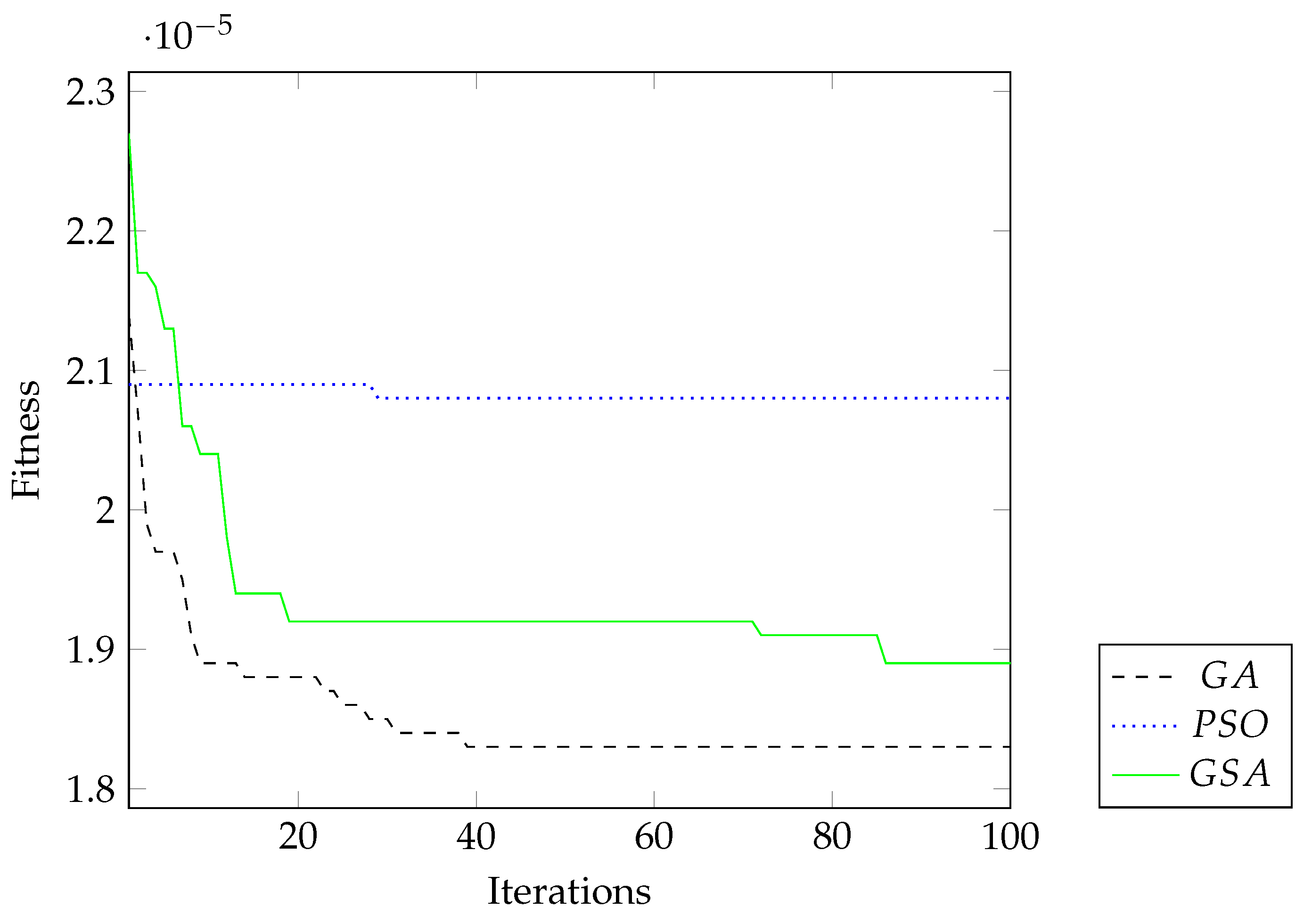
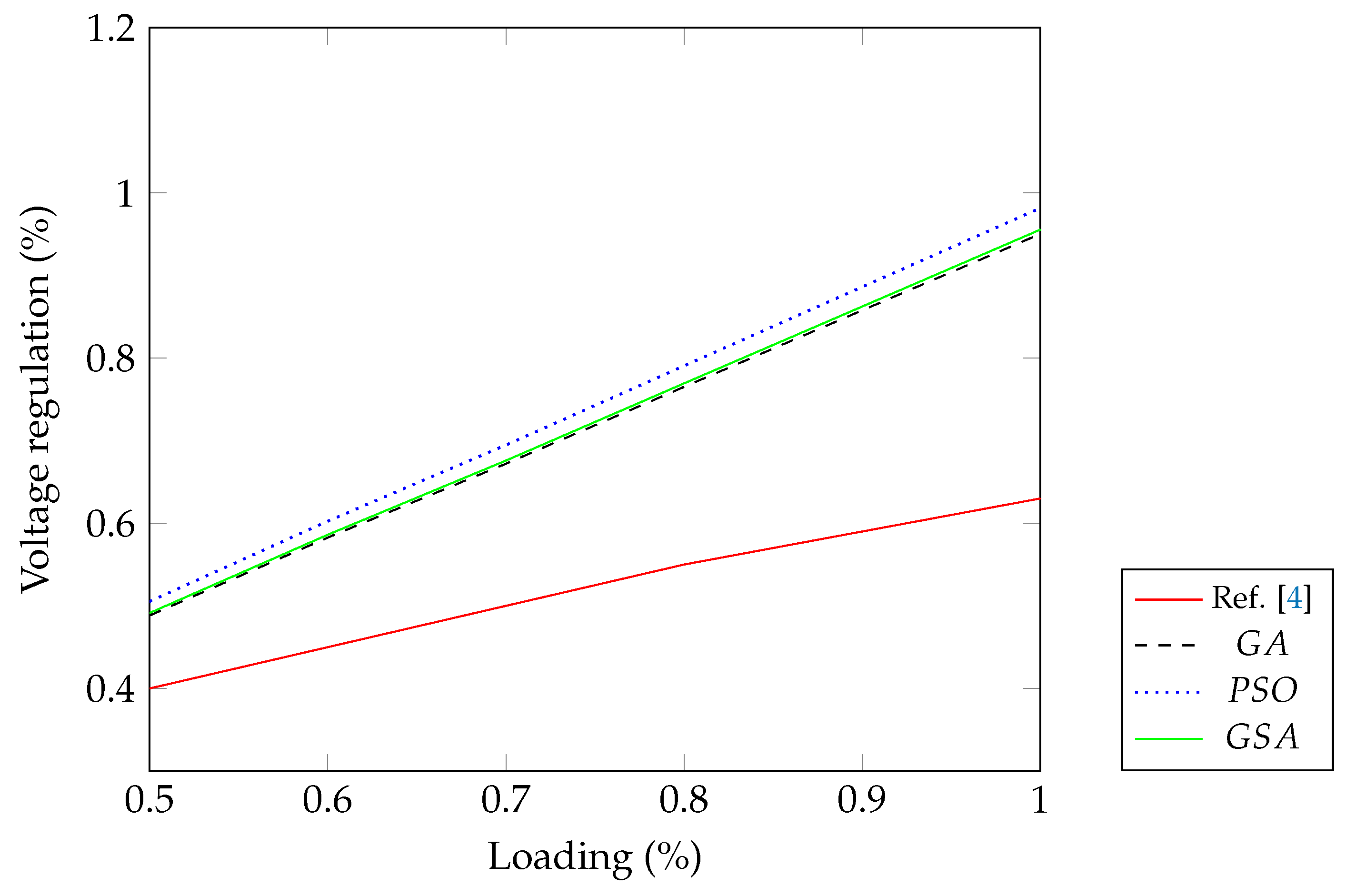
4.2. The Single-Phase Transformer: 15 kVA, 50 Hz, 2400–240 V

Table 4. Statistical values of the SPTECPs using the optimization methods for the single-phase transformer 15 kVA, 2400–240 V at 50 Hz.

	Methods	GA		PSO		GSA
Stats		Fitness	AE (%)	Fitness	AE (%)	Fitness	AE (%)
Best		1.8178 $\times {10}^{-5}$	12.3039	1.92 $\times {10}^{-5}$	11.8855	1.8542 $\times {10}^{-5}$	11.7523
Mean		1.8299 $\times {10}^{-5}$	11.8772	2.0875 $\times {10}^{-5}$	7.8132	1.8936 $\times {10}^{-5}$	9.8612
Medium		1.8305 $\times {10}^{-5}$	12.0800	2.0849 $\times {10}^{-5}$	8.0294	1.8911 $\times {10}^{-5}$	10.9429
Worst		1.8500 $\times {10}^{-5}$	11.7215	2.2897 $\times {10}^{-5}$	8.8045	1.9326 $\times {10}^{-5}$	9.6136
St. dev.		7.4936 $\times {10}^{-8}$	-	8.7936 $\times {10}^{-7}$	-	1.8433 $\times {10}^{-7}$	-
Wilcoxon rank-sum test with 95% confidence				+		+

shows the statistical values and the rank-sum Wilcoxon test results. The sign “+” indicates that the GA is statistically better than PSO and the GSA.

Table 5. Parameters obtained with the optimization methods for the single-phase transformer 15 kVA, 2400–240 V at 50 Hz.

	Parameters	${\mathit{R}}_1(\Omega )$	${\mathit{X}}_1(\Omega )$	${\mathit{R}}_2^{\prime }(\Omega )$	${\mathit{X}}_2^{\prime }(\Omega )$	${\mathit{R}}_{\mathit{c}}(\Omega )$	${\mathit{X}}_{\mathit{m}}(\Omega )$	AE (%)
Methods
Ref. [4]		2.45	3.14	2	2.2294	105,000	9106	-
GA		2.0038	2.5440	1.5060	2.0531	105,730	9176	-
GA error (%)		18.2121	18.9820	24.6983	7.9095	0.6952	0.7662	11.8772
PSO		2.0568	2.9236	1.5504	2.2139	104,473	9130	-
PSO error (%)		16.0503	6.8928	22.48	0.6953	0.5016	0.2595	7.8132
GSA		2.0075	2.7198	1.5103	2.1694	104,453	9103	-
GSA error (%)		18.0612	13.3811	24.4833	2.6913	0.5206	0.0297	9.8612

presents SPTECPs estimated with the optimization methods (the GA, PSO and the GSA). The error obtained by PSO was lower than that obtained in [4]. In case of the GA, there was no difference. Finally, the GSA obtained an error of 4% higher than that in [5].

Table 6. Electrical variables at full load of a single-phase transformer 15 kVA, 2400–240 V, at 50 Hz.

	Variables	${\mathit{I}}_1$ (A)	${\mathit{I}}_2^{\prime }$ (A)	${\mathit{V}}_2^{\prime }$ (V)	Efficiency (%)	AE (%)
Methods
Ref. [4]		6.2	6.2	2383.8	98.5	-
GA		6.2128	6.1834	2377.4751	98.5928	-
GA error (%)		0.2072	0.2673	0.2674	0.0920	0.2085
PSO		6.2113	6.1815	2376.6855	98.5528	-
PSO error (%)		0.1829	0.2983	0.2985	0.0536	0.2083
GSA		6.2130	6.1864	2377.3001	98.5783	-
GSA error (%)		0.2091	0.2187	0.2727	0.0795	0.1950

shows the electrical variables in the single-phase transformer that were estimated with the optimization methods. The reference values of SPTECPs and electrical variables were obtained from [4].

Figure 5 depicts the convergence curves obtained by the GA, PSO and the GSA optimization methods. It is clear that the GA was able to obtain better results in less iterations than the other two methods. The voltage regulation, which was obtained by varying the load, is shown in Figure 6, where the GA, PSO and the GSA results are compared with those obtained in [4]. The GA, PSO and the GSA used the estimated SPTECPs to calculate the voltage. One can observe a considerable difference between the curves at full load, which reduced when the load decreased.

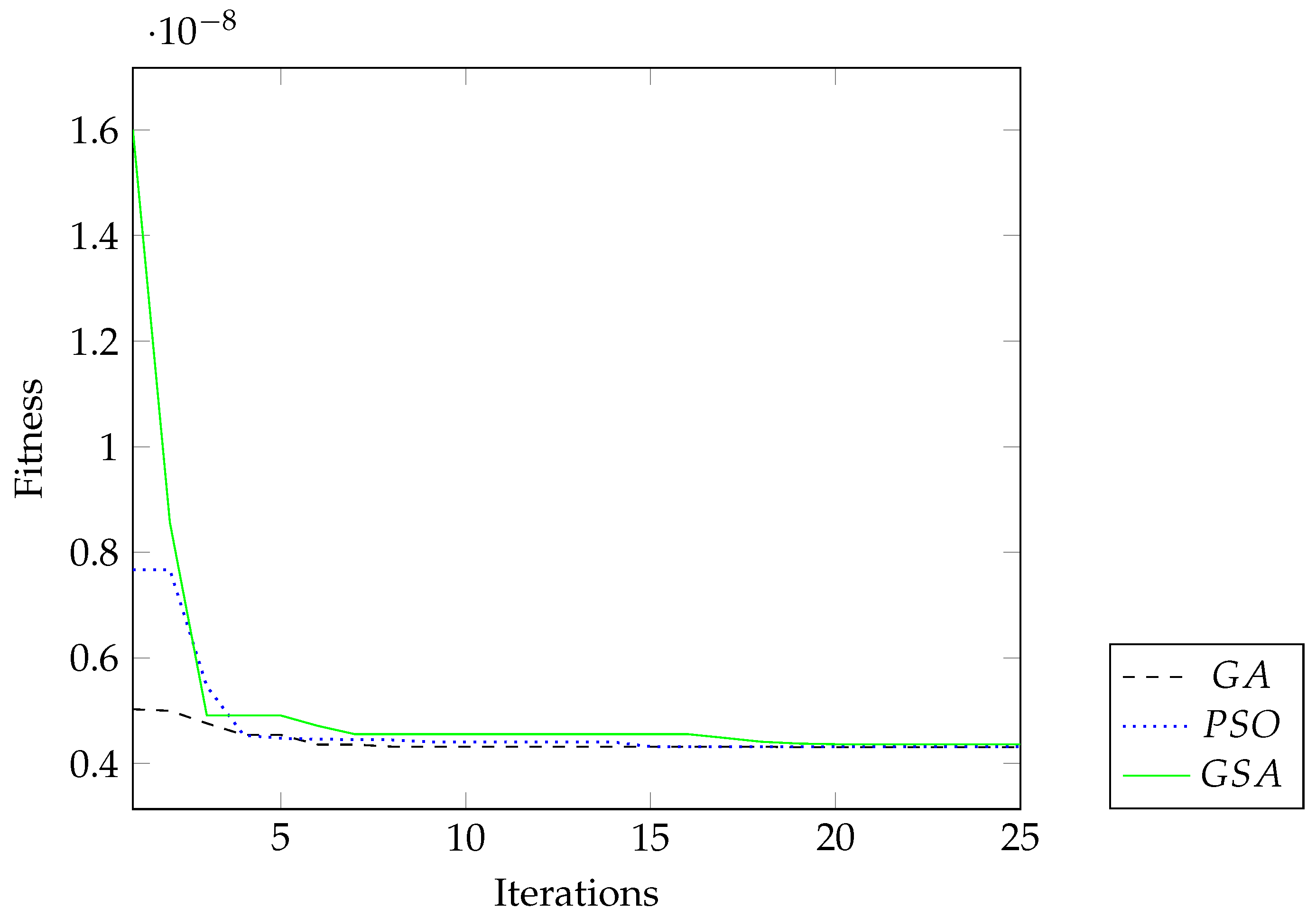
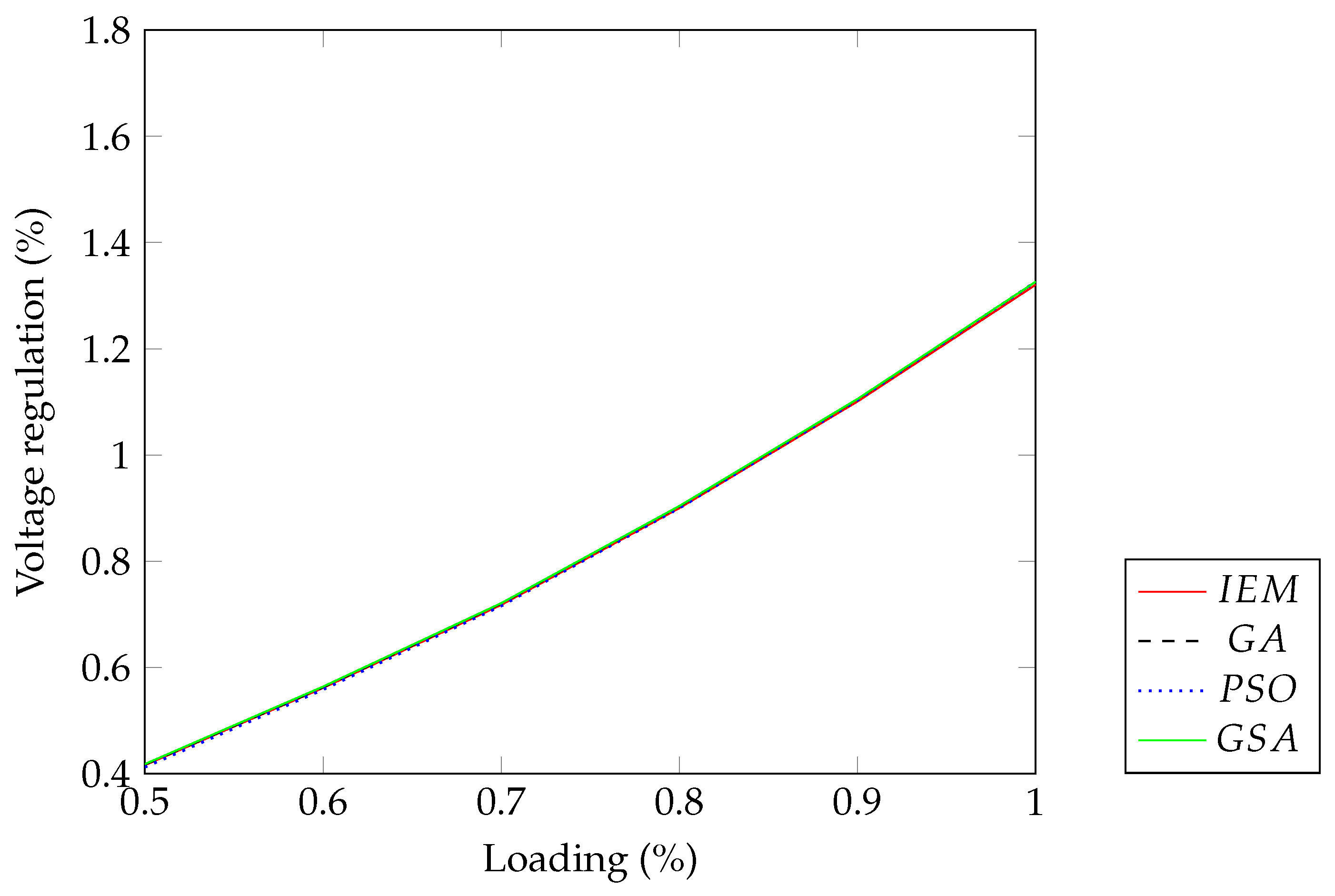
4.3. The Single-Phase Transformer: 33 MVA, 60 Hz, 230,000/$\sqrt{3}$–34,500 V

Table 7. Statistical values of the SPTECPs using the optimization methods for the single-phase transforme 33 MVA, 230,000/$\sqrt{3}$–34,500 V at 60 Hz.

	Methods	GA		PSO		GSA
Stats		Fitness	AE (%)	Fitness	AE (%)	Fitness	AE (%)
Best		4.1138 $\times {10}^{-9}$	8.3152	4.0597 $\times {10}^{-9}$	4.5892	4.1520 $\times {10}^{-9}$	4.5154
Mean		4.2171 $\times {10}^{-9}$	2.6105	4.3105 $\times {10}^{-9}$	1.3703	4.3586 $\times {10}^{-9}$	1.3415
Medium		4.2202 $\times {10}^{-9}$	2.5620	4.3196 $\times {10}^{-9}$	3.3515	4.3646 $\times {10}^{-9}$	3.0648
Worst		4.3153 $\times {10}^{-9}$	3.6331	4.5475 $\times {10}^{-9}$	4.6009	4.5626 $\times {10}^{-9}$	5.4431
St. dev.		5.0994 $\times {10}^{-11}$	-	1.0156 $\times {10}^{-10}$	-	1.1556 $\times {10}^{-10}$	-
Wilcoxon rank-sum test with 95% confidence				+		+

presents the statistical values and the Wilcoxon rank-sum test results for this study case. The sign “+” indicates that the GA is statistically better than PSO and the GSA.

Table 8. Parameters obtained with the optimization methods for the single-phase transformer 33 MVA, 230,000/$\sqrt{3}$–34,500 V at 60 Hz.

	Parameters	${\mathit{R}}_1(\Omega )$	${\mathit{X}}_1(\Omega )$	${\mathit{R}}_2^{\prime }(\Omega )$	${\mathit{X}}_2^{\prime }(\Omega )$	${\mathit{R}}_{\mathit{c}}(\Omega )$	${\mathit{X}}_{\mathit{m}}(\Omega )$	AE (%)
Methods
IEM-Condumex		0.835	37.5	0.835	37.5	728,504	513,610	-
GA		0.8724	38.99	0.8540	35.81	729,277	515,267	-
GA error (%)		4.4790	3.9645	2.2754	4.5155	0.1061	0.3226	2.6105
PSO		0.8105	37.15	0.8074	37.16	727,823	514,097	-
PSO error (%)		2.9341	0.9184	3.2814	0.8995	0.0934	0.0948	1.3703
GSA		0.8408	38.25	0.8002	37.13	727,743	514,170	-
GSA error (%)		0.6946	1.992	4.1677	0.9741	0.1044	0.1090	1.3415

shows SPTECPs estimated with the three optimization methods, where the average error was small.

Table 9. Electrical variables at full load of a single-phase transformer 33 MVA, 230,000/$\sqrt{3}$–34,500 V at 60 Hz.

	Variables	${\mathit{I}}_1$ (A)	${\mathit{I}}_2^{\prime }$ (A)	${\mathit{V}}_2^{\prime }$ (V)	Efficiency (%)	AE (%)
Methods
IEM-Condumex		247.926	247.728	131,060	99.46	-
GA		247.9332	247.7348	131,053.0316	99.4567	-
GA error (%)		0.0025	0.0027	0.0053	0.0033	0.0035
PSO		247.9329	247.7345	131,052.887	99.4765	-
PSO error (%)		0.0028	0.0026	0.0054	0.0166	0.0069
GSA		247.9347	247.7364	131,053.8826	99.4722	-
GSA error (%)		0.0035	0.0034	0.0047	0.0123	0.0060

shows the electrical variables in the single-phase transformer that were estimated with the optimization methods. The reference values of SPTECPs and electrical variables were obtained from IEM-Condumex.

Figure 7 shows the convergence curves of the GA, PSO and the GSA optimization methods. The results are shown only up to the 25th iteration because after that value there was no significant change. In this case, the convergence behavior of the three methods was very similar. The voltage regulation, obtained by varying the load, is shown in Figure 8. The curves obtained using SPTECPs for each optimization method, the GA, PSO and the GSA, are compared in Table 8. In the case of the real single-phase transformer curve, SPTECPs obtained from the open- and short-circuit tests were used.

It can be observed that the error of the results obtained by the evolutionary algorithms, the GA, PSO and the GSA, to estimate the parameters of distribution transformers were larger for distribution transformers than those for power transformers. The reason for this fact lies in the possible error in [4]. Indeed, after substituting the parameters estimated with the algorithms used in [4] and performing an equivalent circuit analysis to obtain the regulation current and voltage, results that differed from those of [4] were obtained.

5. Conclusions

In this work, the efficiency of equivalent circuit parameter estimation, using the GA, PSO and the GSA optimization methods for single-phase power transformers from 4 kVA to 33 MVA, was evaluated. These optimization methods are suitable when the transformer equivalent circuit parameters are not available or when the transformer is in service and cannot be disconnected for open-circuit and short-circuit testing. The three methods compared require only the full-load current and voltage measurements on the windings, as well as the transformer rated capacity. The results obtained for the test systems showed that the average error in the estimation of the equivalent circuit parameters of the single-phase transformer were less than 12%. This accuracy was achieved due to the fact that the fitness values were taken close to zero. In addition, the mean value could serve as a criterion to obtain the best estimate. It was also observed that the SPTECP estimate resulted in a larger error for the distribution transformer than for the power transformer. This was due to some inconsistencies that arose in the calculations in [4], where distribution transformers were analyzed.

As part of our future work, we will apply the differential evolution method to this case study and we will use the metaheuristic optimization methods for estimating parameters of rotating electric machine equivalent circuits (DC electric machines, synchronous machines, induction motors).

References

1. Bigdeli, M.; Azizian, D.; Bakhshi, H.; Rahimpour, E. Identification of transient model parameters of transformer using genetic algorithm. In Proceedings of the 2010 International Conference on Power System Technology, Zhejiang, China, 24–28 October 2010; pp. 1–6. [Google Scholar]
2. Krishan, R.; Mishra, A.K.; Rajpurohit, B.S. Real-time parameter estimation of single-phase transformer. In Proceedings of the 2016 IEEE 7th Power India International Conference (PIICON), Bikaner, India, 25–27 November 2016; pp. 1–6. [Google Scholar]
3. Soliman, S.; Alammari, R.; Mostafa, M. On-line estimation of transformer model parameters. In Proceedings of the 2004 Large Engineering Systems Conference on Power Engineering (IEEE Cat. No. 04EX819), Halifax, NS, Canada, 28–30 July 2004; pp. 170–178. [Google Scholar]
4. Mossad, M.I.; Azab, M.; Abu-Siada, A. Transformer parameters estimation from nameplate data using evolutionary programming techniques. IEEE Trans. Power Deliv. 2014, 29, 2118–2123. [Google Scholar] [CrossRef]
5. Illias, H.A.; Mou, K.; Bakar, A. Estimation of Transformer Parameters from Nameplate Data by Imperialist Competitive and Gravitational Search Algorithms; Elsevier: Amsterdam, The Netherlands, 2017; Volume 36, pp. 18–26. [Google Scholar]
6. Padma, S.; Subramanian, S. Parameter estimation of single phase core type transformer using bacterial foraging algorithm. Engineering 2010, 2, 917. [Google Scholar] [CrossRef]
7. Ćalasan, M.; Mujičić, D.; Rubežić, V.; Radulović, M. Estimation of equivalent circuit parameters of single-phase transformer by using chaotic optimization approach. Energies 2019, 12, 1697. [Google Scholar] [CrossRef] [Green Version]
8. Golberg, D.E. Genetic Algorithms in Search, Optimization, and Machine Learning; Addison-Wesley: Boston, MA, USA, 2002. [Google Scholar]
9. Kennedy, J.; Eberhart, R. Particle swarm optimization. In Proceedings of the ICNN’95-International Conference on Neural Networks, Perth, WA, Australia, 27 November–1 December 1995; Volume 4, pp. 1942–1948. [Google Scholar]
10. Clerc, M.; Kennedy, J. The particle swarm-explosion, stability, and convergence in a multidimensional complex space. IEEE Trans. Evol. Comput. 2002, 6, 58–73. [Google Scholar] [CrossRef] [Green Version]
11. Duarte, C.; Quiroga, J. PSO Algorithm for Parameter Identification in a DC Motor (Spanish); Universidad de Antioquia: Medellín, Colombia, 2010; Volume 55, pp. 116–124. [Google Scholar]
12. Rashedi, E.; Nezamabadi-Pour, H.; Saryazdi, S. GSA: A gravitational search algorithm. Inf. Sci. 2009, 179, 2232–2248. [Google Scholar] [CrossRef]
13. Darzi, S.; Islam, M.T.; Tiong, S.K.; Kibria, S.; Singh, M. Stochastic leader gravitational search algorithm for enhanced adaptive beamforming technique. PLoS ONE 2015, 10, e0140526. [Google Scholar] [CrossRef] [PubMed]
Figure 1. Single-phase transformer equivalent circuit.
Mca 28 00036 g001
Figure 2. Single-phase aproximate transformer equivalent circuit.
Mca 28 00036 g002
Figure 3. Convergence curves of the 4 kVA single-phase transformer using the GA, PSO and the GSA methods.
Mca 28 00036 g003
Figure 4. Voltage regulation by varying the load on the 4 kVA single-phase transformer.
Mca 28 00036 g004
Figure 5. Convergence curves of the 15 kVA single-phase transformer using the GA, PSO and the GSA methods.
Mca 28 00036 g005
Figure 6. Voltage regulation by varying the load on the 15 kVA single-phase transformer.
Mca 28 00036 g006
Figure 7. Convergence curves of the 33 MVA single-phase transformer using the GA, PSO and the GSA methods.
Mca 28 00036 g007
Figure 8. Voltage regulation by varying the load on the 33 MVA single-phase transformer.
Mca 28 00036 g008