Article

Is NSGA-II Ready for Large-Scale Multi-Objective Optimization?

by
Antonio J. Nebro
1,2,
Jesús Galeano-Brajones
3,
Francisco Luna
1,2,* and
Carlos A. Coello Coello
4
1
ITIS Software, University of Málaga, Ada Byron Research Building, 29071 Málaga, Spain
2
Departamento de Lenguajes y Ciencias de la Computación, University of Málaga, E.T.S. de Ingeniería Informática, 29071 Málaga, Spain
3
Departamento de Ingeniería de Sistemas Informáticos y Telemáticos, Universidad de Extremadura, Centro Universitario de Mérida, 06800 Badajoz, Spain
4
Evolutionary Computation Group, CINVESTAV-IPN, Ciudad de México 07360, Mexico
*
Author to whom correspondence should be addressed.
Math. Comput. Appl. 2022, 27(6), 103; https://doi.org/10.3390/mca27060103
Submission received: 26 October 2022 / Revised: 17 November 2022 / Accepted: 28 November 2022 / Published: 30 November 2022

Abstract

:
NSGA-II is, by far, the most popular metaheuristic that has been adopted for solving multi-objective optimization problems. However, its most common usage, particularly when dealing with continuous problems, is circumscribed to a standard algorithmic configuration similar to the one described in its seminal paper. In this work, our aim is to show that the performance of NSGA-II, when properly configured, can be significantly improved in the context of large-scale optimization. It leverages a combination of tools for automated algorithmic tuning called irace, and a highly configurable version of NSGA-II available in the jMetal framework. Two scenarios are devised: first, by solving the Zitzler–Deb–Thiele (ZDT) test problems, and second, when dealing with a binary real-world problem of the telecommunications domain. Our experiments reveal that an auto-configured version of NSGA-II can properly address test problems ZDT1 and ZDT2 with up to 2 17 = 131 , 072 decision variables. The same methodology, when applied to the telecommunications problem, shows that significant improvements can be obtained with respect to the original NSGA-II algorithm when solving problems with thousands of bits.

1. Introduction

Since the publication of the seminal paper of Deb et al. [1] presenting the Non-dominated Sorting Genetic Algorithm-II (NSGA-II) over twenty years ago, this algorithm has become the standard metaheuristic for solving multi-objective optimization problems. Since then, NSGA-II has been included in a large number of works as a reference against which newly proposed approaches are compared (e.g., [2,3,4]). Additionally, it is normally the first-choice solver for dealing with real-world problems [5,6,7,8]. Its popularity can be easily assessed by looking at the number of citations to [1] (e.g., in Google Scholar or Clarivate Analytics).
NSGA-II is a generational genetic algorithm characterized by applying a dominance ranking scheme to foster convergence and the crowding distance density estimator to promote diversity. These components are used in the replacement step prior to building up the population for the next generation of the algorithm. In most of the studies involving NSGA-II, particularly when continuous problems are tackled, it is configured according to a parameterization mimicking the one used when it was originally introduced in [1], namely: population and offspring population size of 100, Simulated Binary Crossover (probability: 0.9, distribution index: 20.0), and Polynomial-based Mutation (probability: 1/L, where L is the number of decision variables of the problem, distribution index: 20.0).
It is well known that the performance of metaheuristics in solving a given problem depends, to a large extent, on its correct parameter settings [9], so the motivation behind this work is to carry out an experimental study to determine to what extent the search capacity of NSGA-II can be improved if it is properly configured. We focus this study on the context of large-scale optimization problems, i.e., those problems having more than 100 decision variables.
The methodology that we have applied consists, first, of using a highly configurable version of NSGA-II, which is available in jMetal, a Java-based optimization framework [10,11]. We assume that any multi-objective genetic algorithm using dominance ranking and the crowding distance in the replacement step is an NSGA-II variant. That version, referred to as AutoNSGA-II, has been made more extensible and flexible so that: (i) it can adopt an external archive to store the non-dominated solutions, (ii) the offspring population size can be different from the population size, and (iii) the variation operators can be taken from an extended set of different crossover and mutation operators besides Simulated Binary Crossover and Polynomial-based Mutation. Second, we use the irace tool [12] to automatically find the best AutoNSGA-II configurations from a set of training instance problems.
We are going to consider two scenarios, one consisting of solving the Zitzler–Deb–Thiele (ZDT) [13] test suite, starting with 2048 decision variables and another one dealing with a real-work binary telecommunication problem where the solutions can have thousands of bits, which aims to minimize the energy consumption and increase the provided bandwidth in an ultra-dense 5G (fifth generation) network. It is important to emphasize that the purpose of this work is not to compare NSGA-II against state-of-the-art algorithms designed to solve large-scale multi-objective problems but to empirically assess up to what extent the performance of NSGA-II can be enhanced when properly configured in the two scenarios previously considered.
The rest of this paper is organized as follows. The next section reviews the related literature and identifies the research gap covered in this work. Section 3 elaborates on the components required to auto-configure NSGA-II with irace, as well as the two target scenarios used to assess the performance of AutoNSGA-II. The results obtained in the experiments conducted are analyzed in Section 4. Finally, Section 5 discusses the main conclusions drawn and proposes some lines for future research.

2. Related Work

The auto-configuration (or auto-tuning) of metaheuristics is an open research field that studies the design of tools that follow the machine learning approach of, given a set of problems used as a training set, automatically finding an accurate parameterization of the algorithm that it is expected to work well on a validation test and, consequently, on similar problems. A further step is the auto-design of metaheuristics, which, given a set of components, is able to create a full algorithm specifically tailored to the training and validation sets. In the field of multi-objective metaheuristics, these issues have been studied in several papers, such as in [14,15,16].
Focusing on NSGA-II, the idea of auto-tuning a configurable version of it by combining jMetal and irace was presented in [17], where the Walking Fish Group (WFG) [18] test suite was used as the training set, and the resulting NSGA-II variant was validated with the same problems plus the Deb–Thiele–Laumanns–Zitzler (DTLZ) [19] test suite. The reported results showed that that version globally outperformed the original NSGA-II in most of the problems when applying four quality indicators. A similar approach has been used in this paper to address large-scale multi-objective optimization problems.
Indeed, the context of large-scale multi-objective optimization is a hot research topic that is mainly motivated because many real-world problems contain hundreds or even thousands of decision variables (e.g., the training of deep neural networks). Consequently, the search space becomes huge and traditional metaheuristics have difficulties finding accurate solutions. One of the first works in this line is [20], where eight multi-objective metaheuristics, including NSGA-II, were tested on the ZDT problems scaling the variables up to 2048. Paper [21] presents a survey of recent proposals, but none of them is based on applying auto-configuration to an existing algorithm.

3. Materials and Methods

In this section, we describe the configurable version of NSGA-II available in jMetal and the experimental methodology adopted, which includes the two scenarios considered, the auto-configuration process with irace, and the computing environments.

3.1. Component-Based NSGA-II

The implementations of NSGA-II in jMetal have evolved over time. Keeping as a reference the behavior of a generic evolutionary algorithm, following the pseudo-code included in Algorithm 1, the first implementation provided by the release presented in [10] was based on a single and large method (130 lines of Java code) that contained all the steps of the algorithm. In the jMetal 5 release [11], this approach was replaced by an abstract class that closely mimicked the pseudo-code, which improved the modularity and reusability of the code. The last implementation, presented in [17], is based on a component-based architecture, where all the steps of an evolutionary algorithm are objects; this scheme offers an enhanced degree of flexibility that allows the generation of evolutionary algorithms in a dynamic way from a repository of components. This architecture is the basis of the AutoNSGA-II algorithm that we will use in this work.
Algorithm 1 Pseudo-code of an evolutionary algorithm.
1:
P ( 0 ) GenerateInitialSolutions()
2:
t 0
3:
Evaluation( P ( 0 ) )
4:
while not TerminationCriterionIsMet() do
5:
    P ( t ) ← Selection( P ( t ) )
6:
    Q ( t ) ← Variation( P ( t ) )
7:
   Evaluate( Q ( t ) )
8:
    P ( t + 1 ) ← Replacement( P ( t ) , Q ( t ) )
9:
    t t + 1
10:
end while
The component types and some of the available instances are shown in Table 1. Therefore, we see that there are three strategies to create a population of solutions: random, Latin hypercube sampling, and the strategy used in some scatter search algorithms (e.g., AbySS [22]). The evaluation of a population can be performed sequentially or in parallel using the processor cores (multithreaded evaluation). We can observe that there are four components to indicate the stopping condition, ranging from the typical computation of a maximum number of evaluations to reach a certain level in a quality indicator; in the latter case, a maximum number of evaluations must also be set to cope with situations where the stopping condition is never fulfilled. The most commonly used selection scheme in NSGA-II is a binary tournament, but we have generalized it to an n-ary tournament and added a random selection. As NSGA-II is a genetic algorithm, the variation component applies both crossover and mutation, and the replacement component characterizing NSGA-II is the one based on ranking and a density estimator.

3.2. Parameter Space for Auto-Configuring NSGA-II

The automatic configuration of our AutoNSGA-II is based on a parameter space that is composed of several elements coming both from the particular selected components and from specific algorithmic parameters. We have to take into account that a number of components are fixed: the evaluation is sequential, the termination is by evaluations, and the replacement is performed based on a ranking procedure (non-dominated sorting) and the use of a density estimator (crowding distance).
Currently, the implementation of AutoNSGA-II can deal with both continuous and binary problems. The full parameter space for solving both types of problems is detailed in Table 2. There is a first group of common parameters that is not dependent on the encoding, and then we include those that are specific for either continuous or binary decision variables.
Given a population size, which we have fixed to 100 solutions, the algorithm can optionally use an external archive to store the non-dominated solutions of capacity 100; in that case, the result of the algorithm will be either the external archive or, otherwise, the population. Furthermore, when using an archive, the population size can vary from 10 to 200, and the crowding distance estimator is used to promote diversity when the archive is full (i.e., the solution having the lowest crowding distance value is removed). While the standard NSGA-II is a generational evolutionary algorithm, we can configure the offspring population size from 1 (i.e., steady-state) to a maximum of 400 solutions.
Next, we describe the parameters for real-coded multi-objective optimization problems. As commented in the previous section, there are three possible strategies for creating the initial population (random, Latin hypercube sampling, and scatter search). The variation component can choose between two crossover operators (SBX and BLX_ALPHA) and four mutation operators (uniform, polynomial, linked polynomial, and non-uniform). The operators can have common parameters (e.g., the crossover probability) and specific parameters (e.g., the distribution index for the SBX crossover is a value in the range [5.0, 400.0]). The mutation probability is problem-dependent, usually set to 1 / n (where n is the number of decision variables), so we consider a mutation probability factor, which is a value between 0.0 and 2.0, in such a way that the effective mutation probability will be the multiplication of that factor and 1 / n . The repair strategies (random, round, bounds) are applied when a variation operator produces values out of bounds:
  • random: the variable takes a random value within the bounds.
  • bounds: if the value is lower/higher than the lower/upper bound, the variable is assigned the lower/upper bound.
  • round: if the value is lower/higher than the lower/upper bound, the variable is assigned the upper/lower bound.
The operators and parameters used to solve binary problems include single-point, HUX, and uniform crossover, while the mutation operator is bit-flip. We have also used here a mutation factor between 0.0 and 2.0 to modulate the effect of the mutation operator.

3.3. Experimental Methodology

Our aim in this paper is to carry out an empirical study to determine if NSGA-II can address large-scale multi-objective optimization problems if it is properly configured. To this end, we designed two trial scenarios (a real-coded benchmark problem and a binary-coded real-world problem) and conducted a set of experiments divided into two phases, namely, auto-configuring NSGA-II with irace with a simple set of instances and performance assessment over a wider testbed.

3.3.1. Scenarios

The first scenario faces continuous benchmark problems; concretely, we have chosen the ZDT instances. These problems were used in the scalability study presented in [20], where a number of algorithms, including NSGA-II, were applied to optimize the problem family configured with up to 2048 variables. In that work, the solvers stopped the search when they found an approximated front whose Hypervolume (HV) was higher than 95% of the HV of the front used as reference. Those algorithms requiring the fewest number of evaluations to fulfill that condition were considered the fastest. A limit of ten million evaluations was also set so that an algorithmic execution reaching such a limit before obtaining an acceptable front was considered unsuccessful. In our scenario, we keep the same stopping condition, but the limit for failed executions is raised to 25 million evaluations and we configure ZDT instances starting from 2048 variables until 131,072 variables.
The second scenario considers a binary real-world problem from the domain of telecommunications, specifically in the context of 5G networks. A key enabling technology for these networks to meet their expected performance in terms of data rates, latency, etc. [23], lies in deploying many small base stations (SBS) close to end-users, which allows better re-use of the electromagnetic spectrum, as well as improving the signal quality and reducing the communication latency [24]. They are known as Ultra-Dense Networks (UDNs). Dimensioned to satisfy a given demand, UDNs incur considerable power consumption because of the number of SBSs that are operating. If no action is taken, this energy consumption also appears even in periods of low demand (e.g., commercial centers, office buildings, out of business hours, etc.). A well-known and standardized approach to reducing the electricity bill is to switch off a subset of the SBSs when they are underutilized. This poses a multi-objective optimization problem, named CSO (cell switch-off), which, given a set of SBSs, has to determine which subset must be turned on/off (binary decision) in order to minimize the power consumption and maximize the capacity provided to the users [25,26,27]. A detailed definition of the problem can be found in Appendix A. Recall that this is a large-scale multi-objective optimization problem, as seminal studies have anticipated that deployments with SBS every few meters might be required [24]. We have scaled up to about 12,000 cells per km 2 in this work. Figure 1 shows an example of a UDN deployment with macro and micro base stations and small cells, where the on-off state of each one corresponds to one bit of the solutions.

3.3.2. Auto-Configuration and Performance Assessment

We now describe the phases of the experiments, namely, the use of irace to approximate the best configurations of AutoNSGA-II and the comparison of the obtained NSGA-II versions with the original one. We would like to point out that irace uses an iterative approach that samples the space of all possible configurations defined in Table 2 according to a particular distribution, selects the best configurations from the newly sampled ones by means of racing, and updates the sampling distribution to bias the sampling towards the best configurations. Therefore, it is a heuristic algorithm that does not guarantee the global optimal algorithmic configuration is found, as the sampling is limited to a maximum number of evaluations for which the algorithm is run with the sampled configuration on a given instance.
In order to use irace, a number of inputs are required:
  • A file describing the parameter space included in Table 2.
  • A set of problems used for training.
  • An executable program that, for each combination of problem and configuration selected by irace, returns an indicator value so that irace can compare different configurations.
  • The total number of different configurations to generate. The default value is 100,000.
In the continuous benchmark problem scenario, common parameters for real-coded variables are used. The training set consists of five ZDT problems with their default number of decision variables: 30 for ZDT1, ZDT2, and ZDT3, and 10 for ZDT4 and ZDT6. The executable is a jar file including jMetal code that, after solving a problem with a particular AutoNSGA-II configuration, applies the hypervolume quality indicator by using a reference front for the problem (as the ZDT are synthetic problems, reference fronts representing a subset of the Pareto fronts are available). Once irace has found a compromised configuration for AutoNSGA-II for the training set, this version of NSGA-II is compared with the original NSGA-II.
In the case of the CSO problem, irace receives the common and binary-coded parameters of Table 2. Evaluating a typical instance of this problem requires a significant amount of time, so generating and evaluating 100,000 configurations is infeasible. Our approach has been to define a small instance (with 1170 bits) that is used for training. As the Pareto front for this problem is unknown, we have defined a reference point (which is the requirement to apply the hypervolume) after inspecting several approximated fronts reached in a number of pilot tests. We have taken the extreme points of these fronts and added an offset in a conservative way to ensure that any approximated front computed by AutoNSGA-II would dominate those points. The reference point is then the result of taking the highest values per dimension of the extreme points. As with benchmark problems, the configuration found for AutoNSGA-II will be compared with the standard NSGA-II on a set of realistic problem instances.

3.3.3. Computing Environments

Running irace for algorithm auto-configuration can require a significant amount of computer power. The experiments on the ZDT problems have been executed in a virtualization environment located at the Ada Byron Research Center at the University of Málaga (Spain). We have used a virtual machine with Intel(R) Xeon(R) Platinum 8358 CPU @ 2.60 GHz processor (64 cores) and 64 GB of RAM. The operating system is Ubuntu 21.04, and the versions of Java and irace are, respectively, JDK 14 and 3.4.1. The version of jMetal is 6.0-SNAPSHOT.
The experimentation conducted on the CSO problem, which is very computationally demanding, has been deployed on the facilities of the Supercomputing and Bioinformatics Center of the Universidad de Málaga, named Picasso. It is a heterogeneous computing platform composed of several clusters with up to 30.616 computing cores. The full hardware description can be found at http://www.scbi.uma.es/site/scbi/hardware, accessed on 25 October 2022. As the stopping condition here is to reach a predefined number of function evaluations because the true Pareto front is not known for this real-world problem, executions can be performed in this heterogeneous environment because runtimes are not relevant for this study. As such, each of these executions is submitted to Picasso using slurm, a cluster job manager, which allocates them to the first available computing core.

4. Results

In this section, we present and analyze the results obtained after applying the experiments in the two scenarios described above.

4.1. ZDT Benchmark

In Table 3, we include the default settings of NSGA-II and the configuration of AutoNSGA-II found by irace. If we compare the two algorithms, we observe that none of the default parameters of NSGA-II is kept by AutoNSGA-II. The auto-configured algorithm uses an external archive with population and offspring populations sizes of 56 and 14, respectively (the default values are 100 in both populations). It is worth noting that the traditionally used Simulated Binary Crossover (SBX) and Polynomial-based Mutation are replaced by BLX_alpha crossover and non-uniform mutation. The configuration obtained by irace sets a value of α = 0.94 for BLX_alpha, which introduces an additional diversity in the population that aims to properly integrate the controlled effect of the non-uniform mutation with the 1 / n scheme used for the mutation rate in the search, and both the perturbation = 0.3 and the mutation factor of 0.45.
We have executed both NSGA-II variants in the first scenario. The results obtained are presented in Table 4, which includes the computing times and evaluations required to reach the stopping condition. It is worth mentioning that we conducted a set of preliminary experiments, which revealed that the computing times and a number of evaluations per algorithm–problem combination were roughly similar, so performing a number of independent runs and reporting mean values would not add relevant information. This has to be taken into account, as it should be noted that some runs take hours or even days to complete. Consequently, the figures in Table 4 are the result of single executions.
If we focus on ZDT1 and 2048 variables, we observe that AutoNSGA-II needs 182,356 evaluations against the 1,250,500 required by NSGA-II. As a consequence, the computing times are reduced from 0.13 to 0.02 h (453 and 87 s, respectively), so the AutoNSGA-II is about 4.6 times faster than NSGA-II. This behavior continues until the number of variables increases up to 16,384, as NSGA-II is unable to solve ZDT1 with 32,768 variables; however, AutoNSGA-II is able to reach an approximated front that satisfies the stopping condition for the 131,072 decision variables of ZDT1 (95% of the HV of the reference front). The figures of ZDT2 are similar to those of ZTD1.
In the case of ZDT3, the number of evaluations decreases for NSGA-II compared to the ones of ZDT1 and ZDT2, while they increase for AutoNSGA-II, which is around 4.2 times faster. For this problem, NSGA-II fails to solve ZDT3 with 32,768 variables, while AutoNSGA-II is not capable of doing so with the largest number of variables. The results for ZDT6 reveal that AutoNSGA-II is about 18 times faster than NSGA-II in solving the problem with up to 65,356 variables, while NSGA-II can only solve it with 8192. The ZDT4 problem deserves special attention. Neither algorithm was able to solve it for 2048 variables, so we decided to re-run the auto-configuration process by using only ZDT4 as the training set. The settings obtained by irace are similar to those shown in Table 3 except for the mutation operator, which is linked polynomial mutation [28] (distributed index = 18.49, mutation probability factor = 0.28, and mutation repair strategy = random). With these parameter values, AutoNSGA-II has been able to solve ZDT4 with 2048 variables in less than 25 million evaluations.
From these results, we can state that the use of auto-configuration for NSGA-II produces a variant that is not only faster than NSGA-II on all problems except for ZDT4 but is also capable of scaling up to more than 100,000 variables in the case of problems ZDT1 and ZDT2, which is a remarkable outcome of our study. Using the five instances as a training set for the auto-configuration process has had the consequence of finding a suitable parameterization for four problems at the expense of a detriment in ZDT4.
The ZDT benchmark was proposed more than 20 years ago, and its problems are considered easy to solve, so we could consider our findings as a kind of lower bound of the capabilities of NSGA-II to solve scalable problems. We could also argue that the time required to solve ZDT1 and ZDT2 with 131,072 variables is more than four days, but we have to consider that we have used virtual machines and we have not applied any optimization technique (e.g., parallelism), so those times could be significantly reduced.

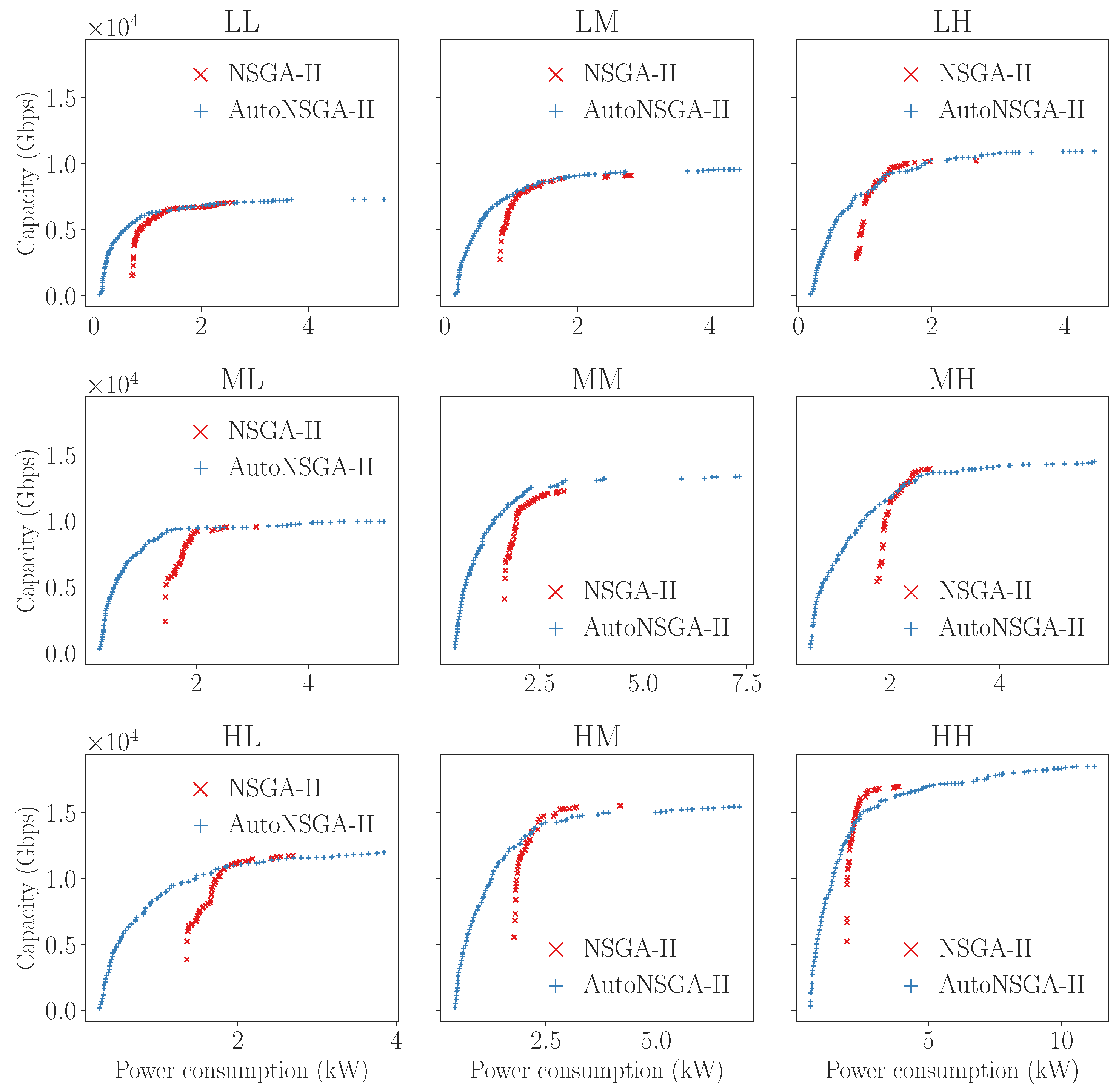
4.2. The CSO Problem

The resulting configuration of AutoNSGA-II and how it contrasts with the typical NSGA-II settings for binary encodings is shown in Table 5. In this case, the main differences are again the presence of an external archive, the size reduction in the two populations (from 100 to 93 and 32 individuals, respectively), almost doubling the mutation impact (to 1.7) and higher selection pressure since a tournament size of 9 is adopted instead of 2.
In this experimental scenario, the goal is not to reach an approximated Pareto front with a given quality level but to approximate the best possible set of non-dominated solutions. To do so, we have used nine different families of CSO instances with an increasing density, not only in the SBSs deployed in the network (i.e., the problem size) but also in the number of existing users that represents the actual demand for data traffic. Three density levels for each parameter have been considered, namely Low, Medium, and High (L, M, and H, respectively), whose full specification is included in Table A1 in the Appendix. The combination of these density levels results in nine families of instances that have already been addressed in previous works [26,27]. We would like to emphasize that we have used the term “family” because the generation of these instances involves random processes for the deployment of both users and SBSs. To address this issue, we have considered here the same 50 random seeds for the two algorithms so that both NSGA-II and AutoNSGA-II face exactly the same generated instances. Two statistical measures of the HV indicator of the approximated Pareto fronts are computed: the mean and the standard deviation (see Table 6). Finally, as we do not have the true Pareto front for this real-world problem, the stopping condition is slightly different from that of the benchmarking problems addressed in the previous section. In fact, a maximum number of function evaluations has been used, which increases with the size of the instances: 100,000, 150,000, and 250,000 for L{X}, M{X}, and H{X}, respectively, with X = {L,M,H}. To obtain a reliable value of the HV indicator, we have first composed a reference Pareto front composed of all the non-dominated solutions found by all the algorithms for each instance, and then we have normalized each approximated front prior to computing the HV value, thus avoiding the effect of the different scaling in the problem objectives.
The HV values reached by NSGA-II and AutoNSGA-II are shown in Table 6, where we have used a gray background to highlight the best (highest) value of the indicator. The conclusion is clear: AutoNSGA-II consistently outperforms NSGA-II in all combinations of densities in the UDN. These differences are remarkable, considering the normalization of the approximated fronts. If we analyze the effect of the density in more detail, we can also observe that when the density of users is Low, i.e., families {X}L (rows 1, 4 and 7), the average HV improvement of AutoNSGA-II is 0.18 over NSGA-II, whereas it is slightly lower for families {X}M and {X}H, which is 0.15 and 0.11, respectively. This showcases a very interesting point for the radio network designer (the decision-maker in the CSO problem) because substantially improved solutions can be reached in periods of very low demand, thus saving more energy consumption. All these results are shown to have statistical significance at a 95% level using either an ANOVA I or a Kruskal–Wallis depending on the normality of the samples, which is checked beforehand by a Kolmogorov–Smirnov test.
In order to better support these claims, in Figure 2, we also show the 50%-attainment surfaces [29] of the nine families of CSO instances. It can be seen that, averaged over all the approximated fronts, the attainment surfaces of AutoNSGA-II cover regions of the solution space with very large energy savings (left-hand side of the plots), where NSGA-II is unable to reach. This particularly holds in the plots of the first column (i.e., families {X}L), corroborating the previous analysis of the HV values. Note that this is a key issue in the deployment of 5G networks, as this problem objective actually computes the instantaneous power consumption, so even small reductions have a deep impact on the electricity bill over a month/year timeframe for a network operator.

5. Conclusions

This work has shown how a well-designed optimization software in combination with an automatic configuration tool such as irace allows tuning the NSGA-II algorithm to deal with large-scale multi-objective optimization problems. By properly adjusting the algorithm components in a methodology that involves not only updating the application rates but also the type of operators used, the auto-configured version of NSGA-II, named AutoNSGA-II, has been successfully evaluated over fairly different scenarios. On the one hand, AutoNSGA-II has been able to address instances of the continuous ZDT problem family (ZDT1 and ZDT2) with up to 2 17 = 131 , 072 decision variables, being considerably faster (in terms of the number of function evaluations and thus the execution time) than the canonical NSGA-II in reaching approximated Pareto fronts with 95% of the HV indicator of the true Pareto front. On the other hand, in a more application-oriented context, AutoNSGA-II has been able to improve upon NSGA-II when addressing a combinatorial optimization problem in ultra-dense 5G networks, where a subset of cells have to be selected to be switched off in order to reach a trade-off between energy consumption and quality of service. The newly algorithmic configuration has been able to reach approximated Pareto fronts with, specifically, higher energy-efficient solutions than those computed by the standard NSGA-II.
A line of work that is worth addressing in the future is to repeat our experiments with the ZDT problems but using each problem separately as a training set aimed at determining, first, whether the performance of AutoNSGA-II can be improved (in terms of reducing the number of evaluations and then reducing the computing time) and, second, to analyze the obtained NSGA-II configurations for each problem to detect common parameter values or components.
The usefulness of using a methodology for automated algorithm tuning, such as NSGA-II, makes sense in the context of dealing with real-world problems, as our study with the CSO has shown. The application of this approach with our combination of jMetal and irace to other problems is also further research work.

Author Contributions

Conceptualization, A.J.N., J.G.-B., F.L. and C.A.C.C.; methodology, A.J.N., F.L. and C.A.C.C.; software, A.J.N. and J.G.-B.; validation, A.J.N., J.G.-B. and F.L.; analysis, A.J.N., J.G.-B., F.L. and C.A.C.C.; writing—original draft preparation, A.J.N. and J.G.-B.; writing—review and editing, A.J.N., J.G.-B., F.L. and C.A.C.C.; All authors have read and agreed to the published version of the manuscript.

Funding

This work has been partially funded by the Spanish Ministry of Science and Innovation via grants PID2020-112540RB-C41 and PID2020-112545RB-C54, by the European Union NextGenerationEU/PRTR under grant and TED2021-131699B-I00 (AEI/FEDER, UE), and the Andalusian PAIDI program with grants P18-RT-2799, A-TIC-608-UGR20, P18.RT.4830, and PYC20-RE-012-UGR. Carlos A. Coello Coello acknowledges support from CONACyT grant no. 2016-01-1920 (Investigación en Fronteras de la Ciencia 2016).

Data Availability Statement

A repository containing the source codes will be publicly available if the paper is accepted.

Acknowledgments

The authors would like to thank Picasso, the supercomputer at the Supercomputing and Bioinformatics centre of the Universidad de Málaga, for providing its services to perform the experiments (http://www.scbi.uma.es/, accessed on 25 October 2022).

Conflicts of Interest

The authors declare no conflict of interest.

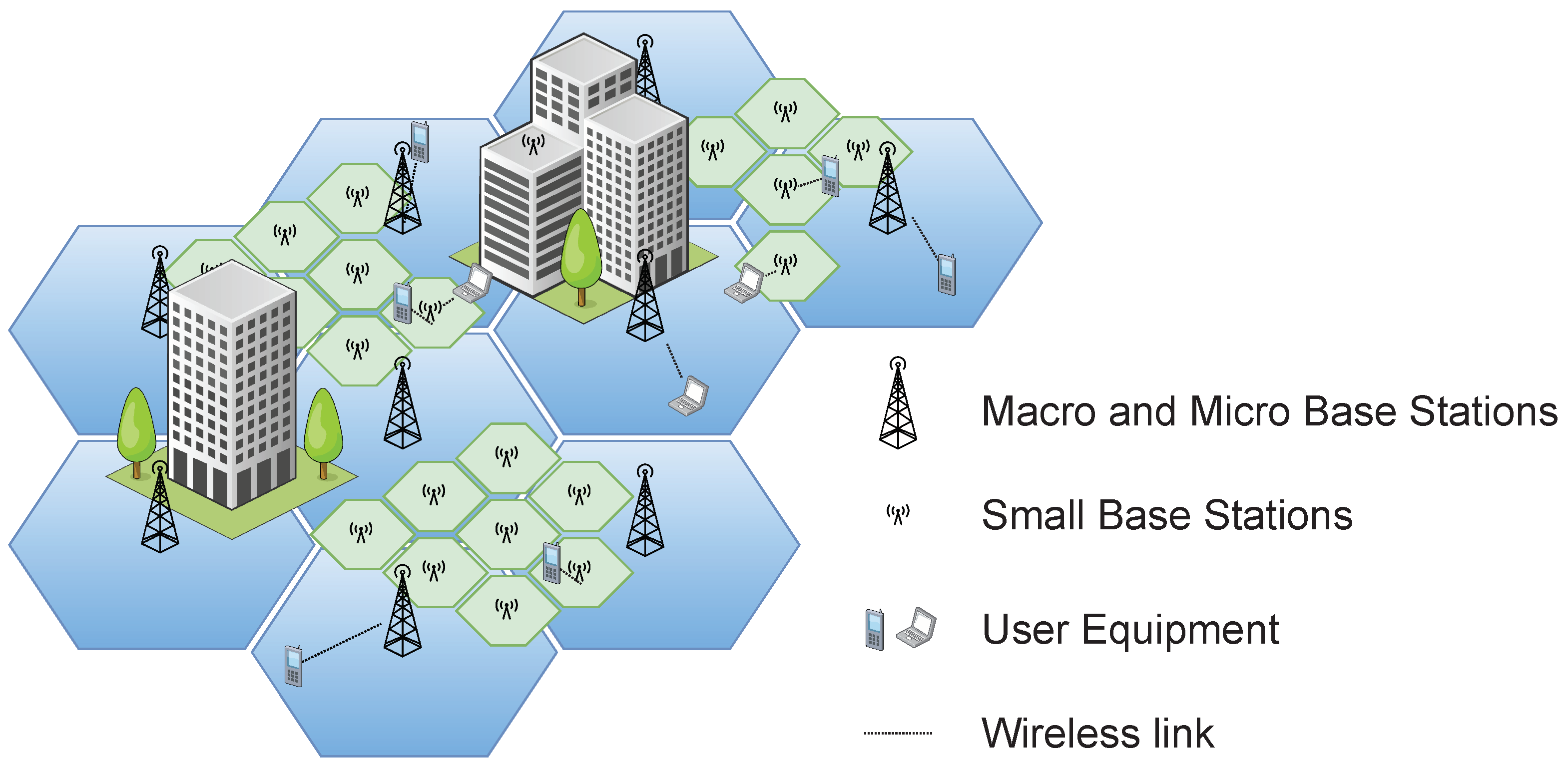
Appendix A. UDN Modeling and Instances

This work considers a service area of 500 × 500 meters, which has been discretized using a grid of 100 × 100 points (also called “pixels” or area elements), each covering a 25 m 2 area, where the signal power is assumed to be constant. In addition to that, vertical densification has been taken into account by considering three vertical area elements, i.e., 25 m of height.
Ten different regions have been defined with different propagation conditions. To compute the received power at each point, P r x [ d B m ] , the following model has been used:
P r x [ d B m ] = P t x [ d B m ] + P L o s s [ d B ]
where P r x is the received power in dBm, P t x is the transmitted power in dBm, and P L o s s is the global signal losses, which depend on the given propagation region, and are computed as:
P L o s s [ d B ] = G A + P A
where G A is the total gain of both antennas, and P A is the transmission losses in space, computed as:
P A [ d B ] = λ 2 · π · d K
where d is the Euclidean distance to the corresponding sector at the SBS, and K is the exponent loss, which randomly ranges in [ 2.0 , 4.0 ] for each of the 10 different regions. The Signal-to-Interference plus Noise Ratio (SINR) for UE k, is computed as:
S I N R k = P r x , j , k [ m W ] i = 1 M P r x , i , k [ m W ] P r x , j , k [ m W ] + P n [ m W ]
where P r x , j , k is the received power by UE k from the cell j, the summation is the total received power by UE k from all the cells operating at the same frequency that j, and P n is the noise power, computed as:
P n [ d B m ] = 174 + 10 · log 10 B W j
where B W j is the bandwidth of cell j, defined as 10% of the SBS operating frequency, which is the same for all the cells it deploys (see Table A1).
Finally, the UE’s capacity has been calculated according to the MIMO depicted in [30]. Thus, we assume that the transmission power from each antenna is P t x / n t x , where n t x indicates the number of transmitting antennas. Then, if we consider the subchannels to be uncoupled, their capacities can add up, and the overall channel capacity of the UE k can be estimated using the Shannon capacity formula:
C k j [ b p s ] = B W k j [ H z ] · i = 1 r log 2 1 + S I N R k · λ i n t x
where λ i is the singular value of the channel matrix H, of dimensions n r x × n t x (i.e., # receiving antennas × # transmitting antennas). Note that both n r x and n t x depend on the cell type (see Table A1). B W k j is the bandwidth assigned to UE k when connected to cell j, assuming a round-robin schedule, that is:
B W k j = B W j N j
where N j is the number of UEs connected to cell j, and the UEs are connected to the cell that provides the highest SINR, regardless of its type.
In order to build a heterogeneous network, three different types of cells of increasing size and decreasing frequency are considered: femtocells, picocells, and microcells. Recall that these cells are generated by the antennas installed in a given sector of an SBS. Figure A1 illustrates the three configurations used in our modeling. In the first row, the three SBSs have the three sectors, and all their cells switched on (in operation). Thus the mapping to the binary string that represents a tentative solution, included below each subfigure, does have all the genes set to 1. In the second row, we have included several solutions with a subset of cells switched off, with the corresponding genes set to 0. It should also be noted that the number of transmitting antennas of each cell type increases with frequency, being 8, 64, and 256 transmitting antennas, respectively, for micro, pico, and femtocells. In the same way, we assume that high-capacity UEs, which will preferably connect to small cells (pico and femtocells), will implement a higher number of receiving antennas (4 and 8 for pico and femtocells, respectively).
Figure A1. Configuration of the SBSs, sectors, and cells used in this work, as well as its mapping into a binary encoded representation.
Mca 27 00103 g0a1
With the system configuration described above, the actual deployment of the cells is carried out via the placement of SBSs in the working area, using a random rotation angle for the sectors, which determines the orientation of the different cell beams. Then, both SBSs and UEs are deployed using independent Poisson Point Processes (PPP) with different densities, defined by λ P C e l l s and λ P U E ), respectively.
The power consumption of a transmitter is computed based on the model presented in [31], which considers that the device is transmitting over the fiber backhauling. Therefore, the regular power consumption of cell j, P j , is expressed as:
P j = α · P + β + δ · S + ρ
where P denotes the transmitted or radiated power of the transmitter, coefficient α represents the efficiency of the transmission power produced by a radio frequency amplifier and feeder losses, the power dissipated due to signal processing and site cooling is denoted by β , and the dynamic power consumption per unit of data is given by δ , where S is the actual traffic demand provided by the serving cell. Finally, the power consumption of the transmitting device is represented by the coefficient ρ . However, in order to consider an accurate power consumption model, the power consumed by the air conditioning and power supply of the SBS should also be taken into account [32]. This has been called maintenance power and is set to 2W/SBS for any SBS containing at least one active cell.
The detailed parametrization of the scenarios addressed is included in Table A1, in which the column equation links the parameter to the corresponding equation in the formulation detailed above. The names in the last nine columns, XY, represent the deployment densities of SBSs and UEs, respectively, so that X = {L, M, H}, meaning either low, medium, or high-density deployments ( λ P C e l l parameter of the PPP), and Y = {L, M, H}, indicate a low, medium, or high density of deployed UEs ( λ P U E parameter of the PPP), in the last row of the table. The parameters G t x and f of each type of cell refer to the transmission gain and the operating frequency (and its available bandwidth) of the antenna, respectively, where n t x and n r x are the number of transmitting and receiving antennas. Finally, the parameters of the previously described power consumption model are also included. Nine instances have been, therefore, used in this work in order to assess the performance of the different metaheuristics and their hybridization with the problem-specific operators.
Table A1. Model parameters for users and base stations.
CellParameterEquationLLLMLHMLMMMHHLHMHH
Micro G t x (A2)12
f(A5)5 GHz (BW = 500 MHz)
α (A8)15
β (A8)10000
δ (A8)1
ρ [ W ] (A8)1
n t x 8
n r x 2
λ P m i c r o ( C e l l s / k m 2 ) 300300300600600600900900900
Pico G t x (A2)20
f(A5)20 GHz (BW = 2000 MHz)
α (A8)9
β (A8)6800
δ (A8)0.5
ρ [ W ] (A8)1
n t x 64
n r x 4
λ P p i c o ( C e l l s / k m 2 ) 150015001500180018001800210021002100
Femto G t x (A2)28
f(A5)68 GHz (BW = 6800 MHz)
α (A8)5.5
β (A8)4800
δ (A8)0.2
ρ [ W ] (A8)1
n t x 256
n r x 8
λ P f e m t o ( C e l l s / k m 2 ) 300030003000600060006000900090009000
UEs λ P U E ( U E / k m 2 ) 100020003000100020003000100020003000

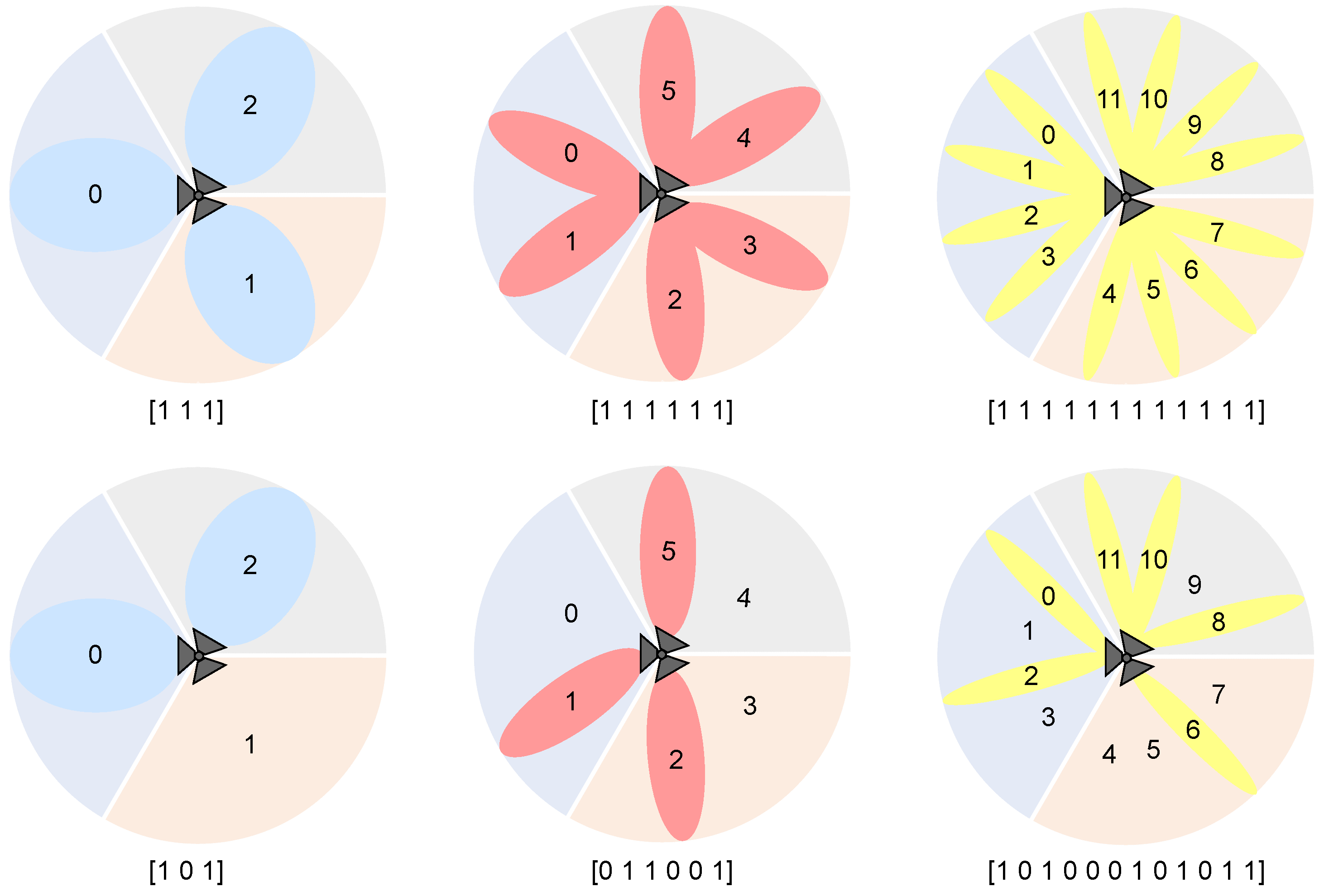
Problem Formulation and Objectives

Let B be the set of randomly deployed SBSs. A solution to the CSO problem is a binary string s { 0 , 1 } B , where s i indicates whether the cell i of a given SBS is activated or not. The first objective to be minimized is, therefore, computed as:
min f P o w e r ( s ) = i = 1 B s i · P i
where P i is the power consumption of SBS i (Equation (A8)). Note that P i includes both the transmission power of every cell i in the SBSs and its maintenance power.
Let U be the set of UEs also deployed, as described in the previous section, and U be the entire set of cells contained in B . Subsequently, in order to compute the total capacity of the system, UEs are first assigned to the active cell that provides it with the highest SINR. Let A ( s ) { 0 , 1 } U × C be the matrix where a i j = 1 if s j = 1 and the Cell j serves UE i with the highest SINR, and a i j = 0 otherwise. Then, the second objective to be maximized, which is the total capacity provided to all UEs, is calculated as:
max f C a p ( s ) = i = 1 U j = 1 C s j · a i j · B W i j
where B W i j is the shared bandwidth of cell j provided to UE i (Equation (A7)). We would like to remark that these two problem objectives are clearly conflicting with each other since switching off base stations leads to a reduction in the power consumption of the network, but it also damages the capacity received by the user, as the UE–cell distance increases (rising the propagation losses) at the same time as the available bandwidth to serve users is reduced.

References

  1. Deb, K.; Pratap, A.; Agarwal, S.; Meyarivan, T. A Fast and Elitist Multiobjective Genetic Algorithm: NSGA-II. IEEE Trans. Evol. Comput. 2002, 6, 182–197. [Google Scholar] [CrossRef] [Green Version]
  2. Li, H.; Zhang, Q. Multiobjective Optimization Problems With Complicated Pareto Sets, MOEA/D and NSGA-II. IEEE Trans. Evol. Comput. 2009, 13, 284–302. [Google Scholar] [CrossRef]
  3. Reyes Sierra, M.; Coello Coello, C.A. Improving PSO-Based Multi-objective Optimization Using Crowding, Mutation and ϵ-Dominance. In Evolutionary Multi-Criterion Optimization; Coello Coello, C.A., Hernández Aguirre, A., Zitzler, E., Eds.; Springer: Berlin/Heidelberg, Germany, 2005; pp. 505–519. [Google Scholar]
  4. Nebro, A.J.; Durillo, J.J.; García-Nieto, J.; Coello, C.A.C.; Luna, F.; Alba, E. SMPSO: A new PSO-based metaheuristic for multi-objective optimization. In Proceedings of the 2009 IEEE Symposium on Computational Intelligence in Multi-Criteria Decision-Making (MCDM 2009), Nashville, TN, USA, 30 March–2 April 2009; pp. 66–73. [Google Scholar] [CrossRef]
  5. Zavala, G.R.; Nebro, A.J.; Luna, F.; Coello, C.A.C. A survey of multi-objective metaheuristics applied to structural optimization. Struct. Multidiscip. Optim. 2014, 49, 537–558. [Google Scholar] [CrossRef]
  6. Becerra, D.; Sandoval, A.; Restrepo-Montoya, D.; Nino, L.F. A parallel multi-objective Ab initio approach for protein structure prediction. In Proceedings of the 2010 IEEE International Conference on Bioinformatics and Biomedicine, Houston, TX, USA, 9–12 December 2010; pp. 137–141. [Google Scholar]
  7. Fang, W.; Guan, Z.; Su, P.; Luo, D.; Ding, L.; Yue, L. Multi-Objective Material Logistics Planning with Discrete Split Deliveries Using a Hybrid NSGA-II Algorithm. Mathematics 2022, 10, 2871. [Google Scholar] [CrossRef]
  8. Turkson, R.F.; Yan, F.; Ahmed Ali, M.K.; Liu, B.; Hu, J. Modeling and multi-objective optimization of engine performance and hydrocarbon emissions via the use of a computer aided engineering code and the NSGA-II genetic algorithm. Sustainability 2016, 8, 72. [Google Scholar] [CrossRef] [Green Version]
  9. Adenso-Díaz, B.; Laguna, M. Fine-tuning of algorithms using fractional experimental designs and local search. Oper. Res. 2006, 54, 99–114. [Google Scholar] [CrossRef] [Green Version]
  10. Durillo, J.; Nebro, A. jMetal: A Java framework for multi-objective optimization. Adv. Eng. Softw. 2011, 42, 760–771. [Google Scholar] [CrossRef]
  11. Nebro, A.; Durillo, J.J.; Vergne, M. Redesigning the jMetal Multi-Objective Optimization Framework. In Proceedings of the Companion Publication of the 2015 Annual Conference on Genetic and Evolutionary Computation (GECCO Companion ’15), Madrid, Spain, 11–15 July 2015; ACM: New York, NY, USA, 2015; pp. 1093–1100. [Google Scholar] [CrossRef]
  12. López-Ibáñez, M.; Dubois-Lacoste, J.; Pérez Cáceres, L.; Stützle, T.; Birattari, M. The irace package: Iterated Racing for Automatic Algorithm Configuration. Oper. Res. Perspect. 2016, 3, 43–58. [Google Scholar] [CrossRef]
  13. Zitzler, E.; Deb, K.; Thiele, L. Comparison of Multiobjective Evolutionary Algorithms: Empirical Results. Evol. Comput. 2000, 8, 173–195. [Google Scholar] [CrossRef] [PubMed] [Green Version]
  14. Blot, A.; Hoos, H.H.; Jourdan, L.; Kessaci-Marmion, M.É.; Trautmann, H. MO-ParamILS: A Multi-objective Automatic Algorithm Configuration Framework. In Learning and Intelligent Optimization; Festa, P., Sellmann, M., Vanschoren, J., Eds.; Springer International Publishing: Cham, Switzerland, 2016; pp. 32–47. [Google Scholar]
  15. Bezerra, L.C.T.; López-Ibáñez, M.; Stützle, T. Automatic Component-Wise Design of Multiobjective Evolutionary Algorithms. IEEE Trans. Evol. Comput. 2016, 20, 403–417. [Google Scholar] [CrossRef] [Green Version]
  16. Bezerra, L.C.T.; López-Ibáñez, M.; Stützle, T. Automatically Designing State-of-the-Art Multi- and Many-Objective Evolutionary Algorithms. Evol. Comput. 2020, 28, 195–226. [Google Scholar] [CrossRef] [PubMed]
  17. Nebro, A.J.; López-Ibáñez, M.; Barba-González, C.; García-Nieto, J. Automatic Configuration of NSGA-II with jMetal and Irace; Association for Computing Machinery, Inc.: New York, NY, USA, 2019; pp. 1374–1381. [Google Scholar] [CrossRef] [Green Version]
  18. Huband, S.; Barone, L.; While, R.; Hingston, P. A Scalable Multi-objective Test Problem Toolkit. In Proceedings of the Third International Conference on Evolutionary MultiCriterion Optimization, EMO 2005, Guanajuato, Mexico, 9–11 March 2005; Coello, C., Hernández, A., Zitler, E., Eds.; Springer: Berlin, Germany, 2005. Lecture Notes in Computer Science. Volume 3410, pp. 280–295. [Google Scholar]
  19. Deb, K.; Thiele, L.; Laumanns, M.; Zitzler, E. Scalable Test Problems for Evolutionary Multiobjective Optimization. In Evolutionary Multiobjective Optimization. Theoretical Advances and Applications; Abraham, A., Jain, L., Goldberg, R., Eds.; Springer: Berlin/Heidelberg, Germany, 2001; pp. 105–145. [Google Scholar]
  20. Durillo, J.J.; Nebro, A.J.; Coello, C.A.C.; Garcia-Nieto, J.; Luna, F.; Alba, E. A Study of Multiobjective Metaheuristics When Solving Parameter Scalable Problems. IEEE Trans. Evol. Comput. 2010, 14, 618–635. [Google Scholar] [CrossRef] [Green Version]
  21. Tian, Y.; Si, L.; Zhang, X.; Cheng, R.; He, C.; Tan, K.C.; Jin, Y. Evolutionary Large-Scale Multi-Objective Optimization: A Survey. ACM Comput. Surv. 2021, 54, 174. [Google Scholar] [CrossRef]
  22. Nebro, A.J.; Luna, F.; Alba, E.; Dorronsoro, B.; Durillo, J.J.; Beham, A. AbYSS: Adapting Scatter Search to Multiobjective Optimization. IEEE Trans. Evol. Comput. 2008, 12, 439–457. [Google Scholar] [CrossRef]
  23. Bohli, A.; Bouallegue, R. How to Meet Increased Capacities by Future Green 5G Networks: A Survey. IEEE Access 2019, 7, 42220–42237. [Google Scholar] [CrossRef]
  24. Lopez-Perez, D.; Ding, M.; Claussen, H.; Jafari, A.H. Towards 1 Gbps/UE in Cellular Systems: Understanding Ultra-Dense Small Cell Deployments. IEEE Commun. Surv. Tutorials 2015, 17, 2078–2101. [Google Scholar] [CrossRef] [Green Version]
  25. González González, D.; Mutafungwa, E.; Haile, B.; Hämäläinen, J.; Poveda, H. A Planning and Optimization Framework for Ultra Dense Cellular Deployments. Mob. Inf. Syst. 2017, 2017, 9242058. [Google Scholar] [CrossRef]
  26. Luna, F.; Luque-Baena, R.; Martínez, J.; Valenzuela-Valdés, J.; Padilla, P. Addressing the 5G Cell Switch-off Problem with a Multi-objective Cellular Genetic Algorithm. In Proceedings of the IEEE 5G World Forum, 5GWF 2018—Conference Proceedings, Silicon Valley, CA, USA, 9–11 July 2018; pp. 422–426. [Google Scholar] [CrossRef] [Green Version]
  27. Luna, F.; Zapata-Cano, P.H.; González-Macías, J.C.; Valenzuela-Valdés, J.F. Approaching the cell switch-off problem in 5G ultra-dense networks with dynamic multi-objective optimization. Future Gener. Comput. Syst. 2020, 110, 876–891. [Google Scholar] [CrossRef]
  28. Zille, H.; Ishibuchi, H.; Mostaghim, S.; Nojima, Y. Mutation operators based on variable grouping for multi-objective large-scale optimization. In Proceedings of the 2016 IEEE Symposium Series on Computational Intelligence (SSCI), Athens, Greece, 6–9 December 2016; pp. 1–8. [Google Scholar] [CrossRef]
  29. Knowles, J. A summary-attainment-surface plotting method for visualizing the performance of stochastic multiobjective optimizers. In Proceedings of the 5th ISDA, Washington, DC, USA, 8–10 September 2005; pp. 552–557. [Google Scholar]
  30. Vucetic, B.; Yuan, J. Performance Limits of Multiple-Input Multiple-OutputWireless Communication Systems. In Space-Time Coding; John Wiley & Sons, Ltd.: Hoboken, NJ, USA, 2005; chapter 1; pp. 1–47. [Google Scholar]
  31. Piovesan, N.; Fernandez Gambin, A.; Miozzo, M.; Rossi, M.; Dini, P. Energy sustainable paradigms and methods for future mobile networks: A survey. Comput. Commun. 2018, 119, 101–117. [Google Scholar] [CrossRef]
  32. Son, J.; Kim, S.; Shim, B. Energy Efficient Ultra-Dense Network Using Long Short-Term Memory. In Proceedings of the 2020 IEEE Wireless Communications and Networking Conference (WCNC), Seoul, Republic of Korea, 25–28 May 2020; pp. 1–6. [Google Scholar]
Figure 1. An example of a UDN.
Mca 27 00103 g001
Figure 2. Attainment surfaces for the nine CSO instance families.
Mca 27 00103 g002
Table 1. Component catalog in jMetal for evolutionary algorithms.
Solutions CreationEvaluationTermination
- Random
- Latin hypercube sampling
- Scatter search
- Sequential
- Multithreaded
- By evaluations
- By time
- By keyboard
- By quality indicator
SelectionVariationReplacement
- N-ary tournament
- Random
- Neighbour
- Differential evolution
- Crossover and mutation
- Differential evolution
- Ranking and density estimator
- ( μ + λ )
- ( μ , λ )
Table 2. Parameter space of AutoNSGA-II for real- and binary-coded problems.
ParameterDomain
algorithmResult{externalArchive, population}
populationSizeWithArchive[10, 200]                                s.t. algorithmResult == externalArchive
externalArchivecrowdingDistanceArchive       s.t. algorithmResult == externalArchive
offspringPopulationSize[1, 400]
selection{tournament, random}
selectionTournamentSize(2, 10)            s.t. selection == tournament
Real-coded variables
createInitialSolutions{random, latinHypercubeSampling, scatterSearch}
variationcrossoverAndMutationVariation
crossover{SBX, BLX_ALPHA}
crossoverProbability[0.0, 1.0]
crossoverRepairStrategy{random, round, bounds}
sbxDistributionIndex[5.0, 400.0]      s.t. crossover == SBX
blxAlphaCrossoverAlphaValue[0.0, 1.0]          s.t. crossover == BLX_ALPHA
mutation{uniform, polynomial, linkedPolynomial, nonUniform}
mutationProbabilityFactor[0.0, 2.0]
mutationRepairStrategy{random, round, bounds}
polynomialMutationDistributionIndex[5.0, 400.0]      s.t. mutation ∈ {polynomial, linkedPolinomial}
uniformMutationPerturbation[0.0, 1.0]          s.t. mutation == uniform
nonUniformMutationPerturbation[0.0, 1.0]          s.t. mutation == nonUniform
Binary-coded variables
createInitialSolutionsrandom
variationcrossoverAndMutationVariation
crossover{singlePoint, HUX, uniform}
crossoverProbability[0.0, 1.0]
mutation{bitflip}
mutationProbabilityFactor[0.0, 2.0]
Table 3. Settings of NSGA-II and AutoNSGA-II for the ZDT problems.
Default Settings for NSGA-IISettings of AutoNSGA-II
algorithmResult: populationalgorithmResult: externalArchive
populationSize: 100populationSizeWithArchive: 56
offspringPopulationSize: 100offspringPopulationSize: 14
variation: crossoverAndMutationVariationvariation: crossoverAndMutationVariation
crossover: SBXcrossover: BLX_ALPHA
crossoverProbability: 0.9crossoverProbability: 0.88
crossoverRepairStrategy: randomcrossoverRepairStrategy: bounds
sbxDistributionIndexValue: 20.0blxAlphaCrossoverAlphaValue: 0.94
mutation: polynomialmutation: nonUniform
mutationProbabilityFactor: 1mutationProbabilityFactor: 0.45
mutationRepairStrategy: randommutationRepairStrategy: round
polynomialMutationDistributionIndex: 20.0nonUniformMutationPerturbation: 0.3
selection: tournamentselection: tournament
selectionTournamentSize: 2selectionTournamentSize: 9
Table 4. Results for NSGA-II and AutoNSGA-II on the ZDT benchmark. The last row shows the time and evaluations of AutoNSGA-II using a specific configuration for the ZDT4 problem.
Time (h)Evaluations
ProblemVariablesNSGA-IIAutoNSGA-IINSGA-IIAutoNSGA-II
ZDT120480.130.021,250,500182,356
40960.510.122,906,100484,356
81922.400.506,622,6001,039,156
16,38411.192.1514,741,2002,180,656
32,768-9.04-4,605,556
65,356-31.66-9,494,556
131,072-120.02-19,359,356
ZDT220480.140.021,472,800164,756
40960.620.103,433,100429,156
81922.770.497,676,600986,556
16,38412.302.2817,059,6002,358,056
32,768-9.28-4,736,056
65,356-39.19-10,081,856
131,072-138.85-21,703,556
ZDT320480.100.031,089,800253,356
40960.470.162,514,200610,956
81922.080.625,463,0001,267,656
16,3849.182.6811,877,5002,820,556
32,768-11.39-6,158,256
65,356-40.69-11,912,856
131,072----
ZDT4 *2048-2.62-21,746,882
ZDT620480.450.045,401,100291,856
40961.820.1611,482,400659,956
81927.160.6624,897,3001,374,056
16,384-3.08-3,221,156
32,768-15.51-7,941,156
65,356-63.79-17,685,556
131,072----
* This instance has used a specifically tuned configuration by irace.
Table 5. Settings for NSGA-II and AutoNSGA-II for the CSO problem.
Default Settings for NSGA-IISettings of AutoNSGA-II
algorithmResult: populationalgorithmResult: externalArchive
populationSize: 100populationSizeWithArchive: 93
offspringPopulationSize: 100offspringPopulationSize: 32
variation: crossoverAndMutationVariatiovariation: crossoverAndMutationVariation
crossover: singlePointcrossover: singlePloint
crossoverProbability: 0.90crossoverProbability: 0.89
mutation: bitFlipmutation: bitFlip
mutationProbabilityFactor: 1mutationProbabilityFactor: 1.7
selection: tournamentselection: tournament
selectionTournamentSize: 2selectionTournamentSize: 9
Table 6. HV indicator for the nine CSO problem families ( Mean ± Standard deviation ).
NSGA-IIAutoNSGA-II
LL 0.733 ± 0.074 0.857 ± 0.041
LM 0.726 ± 0.077 0.834 ± 0.044
LH 0.707 ± 0.116 0.814 ± 0.071
ML 0.619 ± 0.084 0.871 ± 0.030
MM 0.659 ± 0.098 0.843 ± 0.048
MH 0.685 ± 0.099 0.823 ± 0.067
HL 0.699 ± 0.080 0.868 ± 0.034
HM 0.644 ± 0.128 0.792 ± 0.119
HH 0.725 ± 0.103 0.812 ± 0.086
Publisher’s Note: MDPI stays neutral with regard to jurisdictional claims in published maps and institutional affiliations.

