
Modeling of Perforated Piezoelectric Plates

ECE-Paris Engineering School, 37 Quai de Grenelle, CS-71520, CEDEX 15, 75015 Paris, France
Math. Comput. Appl. 2022, 27(6), 100; https://doi.org/10.3390/mca27060100
Submission received: 17 October 2022
/
Revised: 14 November 2022
/
Accepted: 22 November 2022
/
Published: 22 November 2022
(This article belongs to the Special Issue Mathematical and Computational Modelling in Mechanics of Materials and Structures)
Abstract
:In this article, we are interested in the behavior of a three-dimensional model of periodic perforated piezoelectric plate, when the thickness h of the plate and the size of the holes are small. We study the dependence of displacements and electric potential on h and , and give equivalent limits when h and tend towards zero. We compute analytical formulae for all effective properties of the periodic perforated piezoelectric plate.
1. Introduction
Piezoelectric plates and, more generally, structures containing piezoelectric materials are widely used in engineering applications, such as sensors or actuators. The piezoelectric effect is the capacity exhibited by some materials to convert a mechanical deformation to electric field and vice versa. Application to the materials of an electric field produces a mechanical deformation. The increased application of composite and perforated (lattice) piezoelectric materials in ground-breaking Micro–Electro–Mechanical-Systems (MEMS) has stimulated great interest in several studies (see Ikeda [1]).
In the literature, there are several papers concerning modeling on piezoelectric structures. We refer, in particular, to the works of Rahmoune [2,3] and Sene [4,5], who modeled the behavior of a piezoelectric static thin plate not perforated with the thickness h tending to zero. In [6], the authors modeled the thin piezoelectric shell. Kauffman and Saint Jean-Paulin [7] studied the behavior of the displacement when the parameter of the thickness of the plate, period of perforation, and the ration between the width of the bar and the period tended to zero. Figueiredo and Leal [8] used asymptotic analysis to obtain a 2D piezoelectric model.
The present paper is inspired by Rahmoune [2,3], and Sene [4,5], and again, we use the asymptotic analysis and homogenization theory (see [9] or [10]) to derive a reduced piezoelectric model and we give the homogenized system. Explicit formulae of elastic, piezoelectric, and dielectric homogenized coefficients are reported.
2. Setting of the Problem
In this section, we first introduce some notations. Then, we recall the static three-dimensional piezoelectric model of non-homogeneous anisotropic thin plate, and we describe its formulation as a boundary value problem and the variational formulation. Throughout this paper, in the Sobolev space of real-valued functions that are measurable and square summable in with respect to the Lebesgue measure. We use to denote the space of infinitely differentiable functions in that are periodic of Y. The subscript stands for Y-periodic functions in the last variable.
2.1. Geometric of the Medium
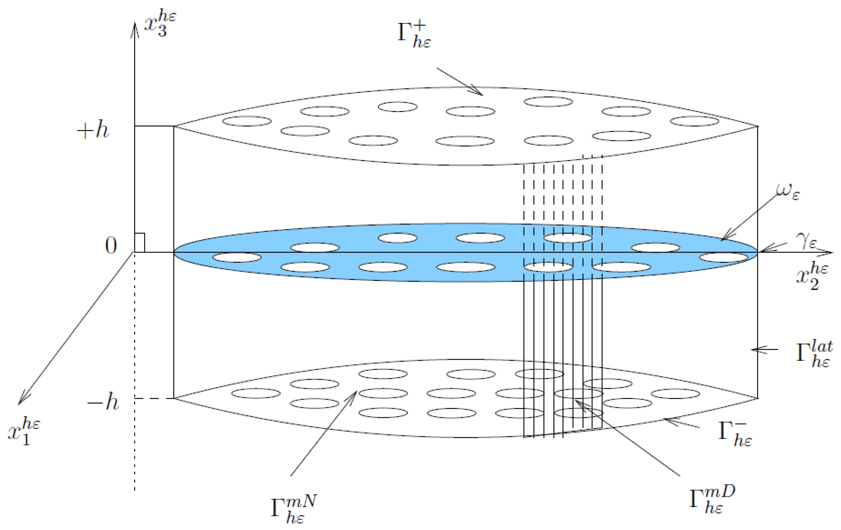
Let be a bounded perforated domain of , the boundary of which is regular. The three dimensional piezoelectric domain is defined in the following way (see Figure 1)
where is plate with middle surface and thickness . is the set of the cylindrical perforations. The upper (resp. lower) face is (resp. ) and is the exterior lateral boundary of the plate. We set
The plate is clamped on the exterior lateral boundary (the Dirichlet conditions) in the placement in with mes We use to denote the complementary portion of the lateral surface. We have
We have Neumann boundary conditions on the boundary of the holes on the top and bottom faces.
2.2. Model Problem
The unknown of the piezoelectric plate model is the pair where denotes the displacement vector field and is the electric potential, which is a scalar field. The current point in is denoted by The plate under consideration is made of linearly piezoelectric and anistropic body; the elastic, piezoelectric and electric moduli are periodic for the variables and . The period is the order of a small-parameter .
The equations of equilibrium and Gauss’s law of electrostatics, in the absence of free charges, are written as:
we complete the boundary conditions,
where (in fact, refers to the restriction of in ). The second-order stress tensor (In the following, we adopt the Einstein convention, with respect to the summation of repeated indices, and the Latin indices run from 1 to Greek indices (except ) taking values in ) and the electric displacement vector are linearly related to the second-order and the scalar electric field by the constitutive law strain tensor
avec , The material properties are given by the fourth-order stiffness tensor measured at constant electric field. The elastic coefficients satisfies the symmetries conditions, and ellipticity uniformly in , and the bounded hypothesis. The coefficients of the third-order piezoelectric tensor (the coupled tensor), verifies the symmetry and bounded conditions. The second-order electric tensor (dielectric permittivity), measured at constant strain, verifies the symmetry and bounded conditions (see [11,12]).
We recall that the variational problem (1)–(3) has a unique solution , corresponding to the saddle point of this functional (see [11,12]):
where
and
In order to study the different limit process (h or tends to zero).
3. The Thin Plate Behavior
We are interested in the limit of three-dimensional problem (1)–(3), when the thickness h of the plate and the period size of holes goes to zero.
3.1. Limit as the Thickness Tends to Zero
The first goal objective is to establish the limit of the three-dimensional variational problem associated with the problem (1) and (2), when We make a suitable choice of the orders of magnitude of the data (4) and (5), and using similar to those of Rahmoune [2] and Sène [4], in order to take into account the presence of holes, we can state the result below, which describes the limiting behavior of the electromechanical state when the thickness h tends to zero.
Theorem 1.
For the piezoelectric variables solution of three-dimensional problem associated the initial problem (1) and (2) defined in . We make the following assumptions about the magnitude of the data with respect to h
where the couple is the element (independent of h) of Moreover, we assume that elastic, electric and piezoelectric constants are independent of We define the scaling of the unknowns:
Then, when the thickness h tends to we obtain
where the limits and satisfy the solution of the variational problem
where
where
is the inverse of matrix
3.2. Limit as the Period Tends to Zero
We now study the limit electrodynamic state when the period of perforation tends to zero. Since the perforated plate has a periodic structure with period , this is a homogenization problem. We denote by x the macroscopic variable and by the microscopic variable. Let us define of periodically perforated subdomains of a bounded open set . The period of is , where is a subset of the unit cube , which represented the solid domain. We use the two-scale convergence approach as introduced by Nguesteng [13] and Allaire [14]; we obtain
Theorem 2.
The sequences , two-scale convergences in , respectively, where is the unique solution of two-scale homogenized problem (Membrane plate equations)
where represents the volume fraction on reference element. The new homogenized law is defined by
The homogenized coefficients and are defined by
we use to denote the mean value over the basic cell The local functions and are -periodic functions in independent of x, with solutions to these two local problems in
where
Furthermore, the sequence is the solution to problem (7) and (8). Two-scale convergence for shows that is unique solution for the two-scale homogenized problem (flexural plate equations):
The homogenized coefficient is described by:
where . The local functions are defined by the solutions of cell problems
The demonstration of Theorem 2 is exactly the same as in Mechkour [12]. We refer to Mechkour [11,12] for details.
The following result complements the two-scale convergence result by providing a strong convergence, which is very useful from a theoretical and numerical point of view. It is based on remarks that are admissible test functions (in the sense of Allaire [14]).
Proposition 1.
The following convergence holds when ε goes to 0
4. Final Remarks
In this paper, we mathematically justify a reduced piezoelectric plate model, and we have rigorously established the limiting equations modeling the behavior of piezoelectric plate in a periodically perforated domain, i.e., we have explicitly described forms of the homogenized coefficients of the elastic, dielectric and coupling tensors.
Funding
This research received no external funding.
Conflicts of Interest
The authors declares no conflict of interest.
References
- Ikeda, T. Fundamentals of Piezoelectricity; Oxford University Press: Oxford, UK, 1990. [Google Scholar]
- Rahmoune, M. Plaques Intelligentes piézoélectriques, modélisation et Application au contrôle santé. Ph.D. Thesis, University of Paris 6, Paris, France, 1997. (In French). [Google Scholar]
- Rahmoune, M.; Benjeddou, A.; Ohayon, R.; Osmont, D. New Thin Piezoelectric Plate Model. J. Intell. Mater. Syst. Struct. 1998, 9, 1017–1029. [Google Scholar] [CrossRef]
- Sène, A. Modélisation Asymptotique de Plaque: Contrôlabilité Exacte Frontière, Piézoélectricité. Ph.D. Thesis, University of Grenoble I, Saint-Martin-d’Hères, France, 1999. (In French). [Google Scholar]
- Sène, A. Modelling piezoeletric static thin plates. Asymptot. Anal. 2001, 25, 1–20. [Google Scholar]
- Ghergu, M.; Griso, G.; Mechkour, H.; Miara, B. Homogenization of thin piezoelectric perforated shells. ESAIM Math. Model. Numer. Anal. 2007, 41, 875–895. [Google Scholar] [CrossRef]
- Kauffman, R.; Saint Jean-Paulin, J. Elasticity of a Perforated Plate with Very Different Elasticity Coeffficients. Gakuto Int. Ser. Math. Sci. Appl. 1997, 9, 225–239. [Google Scholar]
- Figueiredo, N.I.M.; Leal, F.C.M. A piezoelectric anisotropic plate model. Asymptot. Anal. 2005, 44, 327–346. [Google Scholar]
- Cioranescu, D.; Donato, P. An Introduction to Homogenization; Oxford Lecture Series in Mathematics and its Applications; Oxford University Press: Oxford, UK, 1999; Volume 17. [Google Scholar]
- Bensoussan, A.; Lions, J.L.; Papanicolaou, G. Asymptotic Analysis for Periodic Structures; Elsevier: Amsterdam, The Netherlands, 1978. [Google Scholar]
- Mechkour, H. Homogénéisation et Simulation Numérique de Structures Piézoélectriques Perforées et Laminées. Ph.D. Thesis, University of Marne-La-Vallée, Marne-La-Vallée, France, 2004. (In French). [Google Scholar]
- Mechkour, H. Two-scale homogenization of piezoelectric perforated structures. Mathematics 2022, 10, 1455. [Google Scholar] [CrossRef]
- Nguetseng, G. A general convergence result for a functionnal related to the theory of homogenization. SIAM J. Math. Anal. 1989, 20, 608–623. [Google Scholar] [CrossRef]
- Allaire, G. Homogenization and two scale-convergence. SIAM J. Math. Anal. 1992, 23, 1482–1518. [Google Scholar] [CrossRef]
Figure 1.
Perforated piezoelectric plate.

Publisher’s Note: MDPI stays neutral with regard to jurisdictional claims in published maps and institutional affiliations. |
© 2022 by the author. Licensee MDPI, Basel, Switzerland. This article is an open access article distributed under the terms and conditions of the Creative Commons Attribution (CC BY) license (https://creativecommons.org/licenses/by/4.0/).
Share and Cite
MDPI and ACS Style
Mechkour, H. Modeling of Perforated Piezoelectric Plates. Math. Comput. Appl. 2022, 27, 100. https://doi.org/10.3390/mca27060100
AMA Style
Mechkour H. Modeling of Perforated Piezoelectric Plates. Mathematical and Computational Applications. 2022; 27(6):100. https://doi.org/10.3390/mca27060100
Chicago/Turabian StyleMechkour, Houari. 2022. "Modeling of Perforated Piezoelectric Plates" Mathematical and Computational Applications 27, no. 6: 100. https://doi.org/10.3390/mca27060100