Article

An Efficient Orthogonal Polynomial Method for Auxetic Structure Analysis with Epistemic Uncertainties

1
School of Traffic & Transportation Engineering, Central South University, Changsha 410082, China
2
School of Mechanical Engineering, Southeast University, Nanjing 211189, China
*
Author to whom correspondence should be addressed.
Math. Comput. Appl. 2022, 27(3), 49; https://doi.org/10.3390/mca27030049
Submission received: 15 April 2022 / Revised: 21 May 2022 / Accepted: 25 May 2022 / Published: 2 June 2022

Abstract

:
Traditional approaches used for analyzing the mechanical properties of auxetic structures are commonly based on deterministic techniques, where the effects of uncertainties are neglected. However, uncertainty is widely presented in auxetic structures, which may affect their mechanical properties greatly. The evidence theory has a strong ability to deal with uncertainties; thus, it is introduced for the modelling of epistemic uncertainties in auxetic structures. For the response analysis of a typical double-V negative Poisson’s ratio (NPR) structure with epistemic uncertainty, a new sequence-sampling-based arbitrary orthogonal polynomial (SS-AOP) expansion is proposed by introducing arbitrary orthogonal polynomial theory and the sequential sampling strategy. In SS-AOP, a sampling technique is developed to calculate the coefficient of AOP expansion. In particular, the candidate points for sampling are generated using the Gauss points associated with the optimal Gauss weight function for each evidence variable, and the sequential-sampling technique is introduced to select the sampling points from candidate points. By using the SS-AOP, the number of sampling points needed for establishing AOP expansion can be effectively reduced; thus, the efficiency of the AOP expansion method can be improved without sacrificing accuracy. The proposed SS-AOP is thoroughly investigated through comparison to the Gaussian quadrature-based AOP method, the Latin-hypercube-sampling-based AOP (LHS-AOP) method and the optimal Latin-hypercube-sampling-based AOP (OLHS-AOP) method.

1. Introduction

In the analysis of structural geometric nonlinearity and large-deformation engineering practice, experimental tests and finite element computational simulations are two important methods used for analyzing the structural mechanics properties. In the last few years, a large number of thin-walled structures [1,2,3] and auxetic structures [4,5,6,7,8] have been designed for improving the safety in the automotive, railway, and aerospace industries because of their unconventional mechanical properties. Considering the fact that structural large deformation is a complicated dynamic problem, the material properties and structural geometric design will influence the mechanical properties, for example, the modulus of elasticity, tensile strength, stiffness, elongation, hardness and fatigue limit. The analysis of the mechanical properties of traditional structures is still limited to the analysis of deterministic parameters. In engineering practice, uncertainties exist in manufacturing production, usually based on material properties, structural geometric size, boundary conditions, complicated loads, etc. [9,10,11]. Although these uncertainties are small in value, for complicated large-deformation problems with strong nonlinear properties, uncertainty may cause performance to deviate significantly from that expected or even lead to structural failure under coupling [12,13,14]. Recently, some researchers have employed uncertain analysis methods to handle interval or randomness problems for the analysis of thin-walled structures and some traditional structures [15,16,17,18,19,20,21].
Based on the nature of uncertain sources, uncertainty can be divided into the categories of epistemic and aleatory uncertainty [22,23]. Aleatory uncertainty is an inherent characteristic of the behavior of a system or its environment and is also called objective uncertainty. Aleatory uncertainty is usually modelled by probability theory. In contrast to aleatory uncertainty, epistemic uncertainty results from the lack of sufficient knowledge for quantifying an uncertain system. To handle the problems of epistemic uncertainty, several non-probability theories have been developed, including convex models [24], fuzzy sets [25], interval analysis [26,27,28,29], and evidence theory [30,31]. In the uncertainty analysis of the evidence theory model, the belief function ( B e l ) and plausibility function ( P l ) are introduced to describe the degree of uncertainty of systems; these are calculated using imprecise basic probability assignment, where the upper and lower probability boundaries of each interval are used to describe the uncertainty of a problem [32]. Compared with the other epistemic model, the framework of evidence theory is more flexible [33]. If the upper and lower boundary of an interval are the only information which can be obtained, the process of uncertainty analysis by evidence theory can be equivalent to the interval analysis. Meanwhile, evidence theory can also be equivalent to probability theory when the probability information of uncertain parameters is sufficient [34]. Due to these typical advantages, evidence theory has gained great popularity in the uncertainty analysis of structures or systems in recent years [35,36,37,38].
In evidence theory, the process of analysis of extreme values of each focal element represents a great computational burden, especially for multidimensional problems. In recent years, large numbers of studies have been devoted to improving the computational efficiency of extreme value analysis in the uncertainty analysis of evidence theory. The interval perturbation method is used for the extreme value analysis of each focal element [39,40,41]. Despite the fact that the interval perturbation method can receive a better computational efficiency than the Monte Carlo simulation method, with the number of focal elements increasing, the computational burden of the perturbation analysis method will inevitably increase as all joint focal-element intervals will be analyzed by interval perturbation method. Recently, the global surrogate model has been employed in evidence-theory-based uncertain analysis, which can reduce the computational cost. In the global surrogate method, the system response can be approximated by establishing a surrogate model, thus improving the computational efficiency of the extreme value analysis of all joint focal elements. Originally, the global surrogate models were applied to the evidence theory model [42,43,44]. Subsequently, Jacobi polynomial expansion was introduced to calculate acoustic system response in the context of evidence theory [45]. Additionally, the Gegenbauer series expansion method [46,47] has been applied to calculate the boundary of expectation and variance in structural acoustic problems. Wang et al. [48] combined evidence theory with the sample-based Legendre-type polynomial method to reduce the computational cost for mechanical systems. Based on the above research, the orthogonal polynomial expansion method has been applied in engineering practice to deal with uncertain analyses of evidence theory. According to the author’s research, the polynomial basis can influence the accuracy of the global surrogate model established by orthogonal polynomial expansion. The arbitrary polynomial chaos expansion method has been applied to the uncertain analysis of acoustic problems with interval and random variables [49]. Compared with the traditional orthogonal polynomial expansion method, the computational error of the arbitrary polynomial chaos method can be greatly reduced by the selection of the optimal weight function without scarifying computational efficiency [50].
As mentioned previously, great developments have been achieved in the field of evidence-theory-based uncertainty quantification. However, some important issues remain unresolved. Firstly, the application of evidence theory in the field of auxetic structures with large deformation has not previously been reported. Recently, the interval model and random model were introduced for the analysis of thin-walled structures, but these two kinds of uncertain models are not suitable for uncertain problems with imprecise probability [14]. The evidence theory has a strong ability to deal with imprecise probability; thus, in this paper, the evidence theory will be applied to the design of complex auxetic structures. Secondly, although the convergence rate of the arbitrary orthogonal polynomial expansion method is faster than that of other orthogonal polynomial expansion methods, its tremendous computational burden still limits its application to uncertain problems when the number of epistemic uncertain parameters is large. The Gaussian quadrature is used to calculate the expansion coefficient of the evidence-theory-based arbitrary orthogonal polynomial expansion method; consequently, the sample points are the tensor products of Gaussian integration points. In other words, the sample points will increase exponentially as the number of variables increases, which can lead to establishing the surrogate model by arbitrary orthogonal polynomial expansion having tremendous computational costs. In engineering practice, mechanical properties are usually accompanied by a large number of uncertainty parameters. For example, the widely used negative Poisson ratio (NPR) periodic structures are commonly composed of many cells, where each cell may contain multiple uncertainty parameters. Therefore, it is necessary to develop an appropriate uncertainty analysis method for use in multivariate auxetic structures with the evidence theory model, especially for periodic auxetic structures.
The aim of this research is to propose a sequence-sampling-based arbitrary orthogonal polynomial (SS-AOP) expansion approach for use in the evidence-theory-based uncertainty analysis of auxetic structural mechanics properties with epistemic uncertainties. In SS-AOP, the response analysis of auxetic structural mechanics properties is approximated by the AOP method, and a new sampling technique is employed to reduce the sampling points, which are used to calculate the expansion coefficients [51,52]. In this sampling technique, the candidates are the Gauss points associated with the optimal Gauss weight function for each evidence variable. Then, by using sequential sampling scheme, the sampling points can be sequentially and uniformly selected from the candidate Gauss points. Finally, the least squares method is used to calculate the expansion coefficients of the SS-AOP expansion method. Based on the proposed SS-AOP, the extreme value of focal elements can be calculated efficiently. Several mathematical test functions and a case of application of the analysis of the mechanics properties of double-V NPR are used to show the computational accuracy and efficiency of the proposed approach in comparison to the conventional sampling method of traditional arbitrary polynomial expansion [39] (this method will be called traditional AOP in the rest of this paper), the Latin-hypercube-sampling-based arbitrary polynomial (LHS-AOP) expansion method and the optimal-Latin-hypercube-sampling-based arbitrary polynomial (OLHS-AOP) expansion method.

2. Epistemic Uncertainty Analysis of Auxetic Structure in Large Deformation with Evidence Theory

This section will describe the application of evidence theory in the mechanics property analysis of auxetic structures. Additionally, the basic conceptions of evidence theory will be briefly introduced.

2.1. Static Analysis with Uncertain Parameter

For the static analysis of complex auxetic structures, the compression process is a highly discontinuous and nonlinear problem. Generally, structural finite element analysis is suitable for solving geometric nonlinear compression problems. For the nonlinear large-deformation problem with systems of multiple degrees of freedom, the structural statics equation can be formulated as
[ K ] { u } + F = 0 ,
where { u } is the displacement vector of each node of the system, K stands for the stiffness matrix, and F denotes the external input matrix.
In real engineering practice in the structural mechanical research field, many uncertainties are inherent. For example, there is uncertainty regarding material properties and the geometric size of auxetic structures caused by manufacturing precision or assembly technology. In addition, the precise probability distribution of these uncertain variables is hard to obtain due to the experimental cost. In this paper, we will use the evidence theory to establish an effective model for auxetic dynamic analysis.
The uncertain variables of auxetic structure can be represented by evidence variables vector U . The dynamic equilibrium equation with evidence variables is formulated as:
[ K ( U ) ] { u } + [ F ( U ) ] = 0 .
In the above equation, the K ( U ) , F ( U ) denote the uncertain-but-bound mass and external excitation matrix, respectively.

2.2. Fundamental Conception of Evidence Theory

In the evidence theory, the universal set Ω of each probable for the uncertainty problem is called the frame of discernment (FD). For instance, if the FD is given as Θ = { x 1 , x 2 } , the x 1 and x 2 are defined as two mutually exclusive elementary propositions. The FD of this example is 2 Θ = { , { x 1 } , { x 2 } , { x 1 , x 2 } } . Additionally, the basic probability assignment (BPA) of an unknown event can be indicated by a function m: 2 Θ [ 0 , 1 ] . For a given event Q, the BPA can be written as:
{ m ( Q ) 0 , Q 2 Θ m ( ) = 0 A 2 Θ m ( Q ) = 1 ,
where each subset m ( Q ) is called the focal element in evidence theory, which satisfies m ( Q ) > 0 .
Due to lack of precise information or knowledge, the deterministic probability information of any proposition B can be obtained in evidence theory. Therefore, an interval which includes B e l and P l will be employed to represent the uncertainty probability of the proposed problem. These measures are defined as:
{ B e l ( B ) = Q B m ( Q ) P l ( B ) = Q B 0 m ( Q ) .
The B e l ( B ) is the probability lower boundary of the proposition B and the P l ( B ) is the upper boundary of the proposition B, where both [ 0 , 1 ] . The belief measure B e l ( B ) is calculated by the summation of the BPA of proposition B, which is wholly contained within proposition B and represents the minimum possibility which can be correlative with proposition B, while the plausibility measure P l ( B ) is calculated by summing the BPA of proposition B, which is completely or partially contained in the proposition B and it represents the maximum possibility which is related to proposition B. The B e l and P l , regarded as the upper and lower probability interval, describe the uncertainty of problems. The probability of a proposition is contained by B e l and P l .

2.3. Establishing Uncertainty Model by Evidence Theory

According to the Ref. [53], each uncertain variable contains one or more than one interval. For example, by using the evidence theory, an uncertain variable U can be expressed as:
U = { ( U 1 I , m ( U 1 I ) ) , , ( U i I , m ( U i I ) ) , , ( U l I , m ( U l I ) ) } ,
where U i I stands for the i th focal element and m ( U 1 I ) represents the BPA of U i I . These focal elements can be regarded as several intervals which may be overlapping or have gaps when there is more than one uncertain variable.
For the multidimensional problem U = { [ U 1 , U 2 , , U k ] } , the joint focal elements can be expressed as
U S k = [ U S 1 , 1 I , U S 2 , 2 I , , U S k , k I ] U 1 × U 2 × U K , S k = 1 , 2 , , N s .
The U S k represents the S k nd joint focal element. Each U S k , k I U i I means the focal element of each evidence variable U i , while N s is the total number of joint focal elements. The joint BPA of U S k is expressed as:
m ( U S k ) = { j = 1 k m ( U S k , i l ) , U S k , k I U i I 0 , e l s e .
According to the definition of the evidence theory model given above, the precise information of the probability distribution of uncertain parameters is not required. For the evidence theory model, the uncertain analysis model still can be established without assumptions. The precise probability density function can be obtained because of the lack of information regarding an uncertain parameter.

3. SS-AOP for Epistemic Uncertainty Analysis under Evidence Theory

According to the traditional AOP expansion method, the number of sampling points increases exponentially along with the expansion order, leading to the global surrogate model requiring a great deal of computational time. This paper proposes a new SS-AOP expansion method to improve the efficiency of the uncertainty analysis of the evidence theory model. In SS-AOP, a new sampling technique is employed to reduce the sampling points; this technique is used to calculate the expansion coefficients of AOP expansion. Firstly, the candidate points for sampling are generated using the Gauss points associated with the optimal Gauss weight function for each evidence variable. Then, the sequential-sampling technique is introduced to select the sampling points from the candidate points. The procedure of the proposed SS-AOP approach will be deduced in this section.

3.1. Fundamentals of Traditional AOP Expansion

The function Y ( ε ) is approximated as:
Y ( ε ) = i = 0 N f i φ i ( ε ) ,
N is the maximum retained order of AOP expansion. f i represents the expansion coefficient, and φ i ( ε ) , ( i = 1 , 2 , L ) denotes the polynomial basis of order i .
According to Ref [54], the polynomial basis is determined as:
φ 1 ( ε ) = 0 φ 0 ( ε ) = 1 φ k + 1 ( ε ) = ( ε a k ) φ k ( ε ) b k φ k 1 ( ε ) , k = 0 , 1 , 2 , .
In Equation (9), a k and b k ( k = 0 , 1 , 2 , ) indicate the recurrence coefficient of the AOP. The procedure to determine the coefficients f i can be found in Ref. [50].
In traditional AOP [50], for the problem of uncertainty caused by multiple parameters, Y ( ε ) can be expressed as:
Y ( ε ) = i 1 = 0 N 1 i L = 0 N L f i 1 , i L φ i 1 , i L ( ε ) ,
where ε = [ ε 1 , ε 2 , , ε L ] is a L -dimensional vector and N i ( i = 1 , 2 , , L ) indicates the retained order of each uncertain variable. φ i 1 , i L ( ε ) can be expressed by:
φ i 1 , i L ( ε ) = j = 1 L φ i j ( ε j ) j = 1 , 2 , , L i j = 1 , 2 , ,
where φ i j ( ε j ) ( j = 1 , 2 , , L ) denotes the polynomial basis associated with ε j , and i j indicates the order of the polynomial basis φ i j ( ε j ) .
According to Ref. [50], the coefficient f i 1 , i L can be expressed as:
f i 1 , i L = 1 h i 1 , , i L Ω Y ( ε ) φ i 1 , , i L ( ε ) w i 1 , , i L ( ε ) d ε   = 1 h i 1 , , i L j 1 = 1 m 1 j L = 1 m L Y i 1 , , i L ( ε ^ j 1 , , j L ) φ j 1 , , j L ( ε ^ j 1 , , j L ) w j 1 , , j L
In the above equations, ε ^ j k indicates the j k nd integration points for ε k , w j k is the weight of Gauss integration related to ε ^ j L and m k ( k = 1 , 2 , , L ) is the total number of integration nodes related to ε k . In order to ensure the efficiency and accuracy of the AOP method, the number of Gauss integration points m k will be set as m k = n i + 1 .
According to Equation (12), for multidimensional problems, the number of polynomial basis and integration points will increase exponentially with an increase in retain order n i . To improve the computational efficiency, a new sampling technique will be developed for the calculation of the expansion coefficient in the following section.

3.2. The Sequence Sampling Scheme

The most widely used sampling technique is Latin hypercube sampling (LHS). However, the LHS-based method generates sampling points that are approximately random, which may lead to the calculation results being unreliable. In this section, a new sequence sampling approach is developed. Firstly, the candidate points for sampling are generated using the Gauss points associated with the optimal Gauss weight function for each evidence variable. This is because the Gauss points have a great influence on the convergence and accuracy. Secondly, the sequence sampling approach will be introduced to uniformly select the sampling points from candidate points.

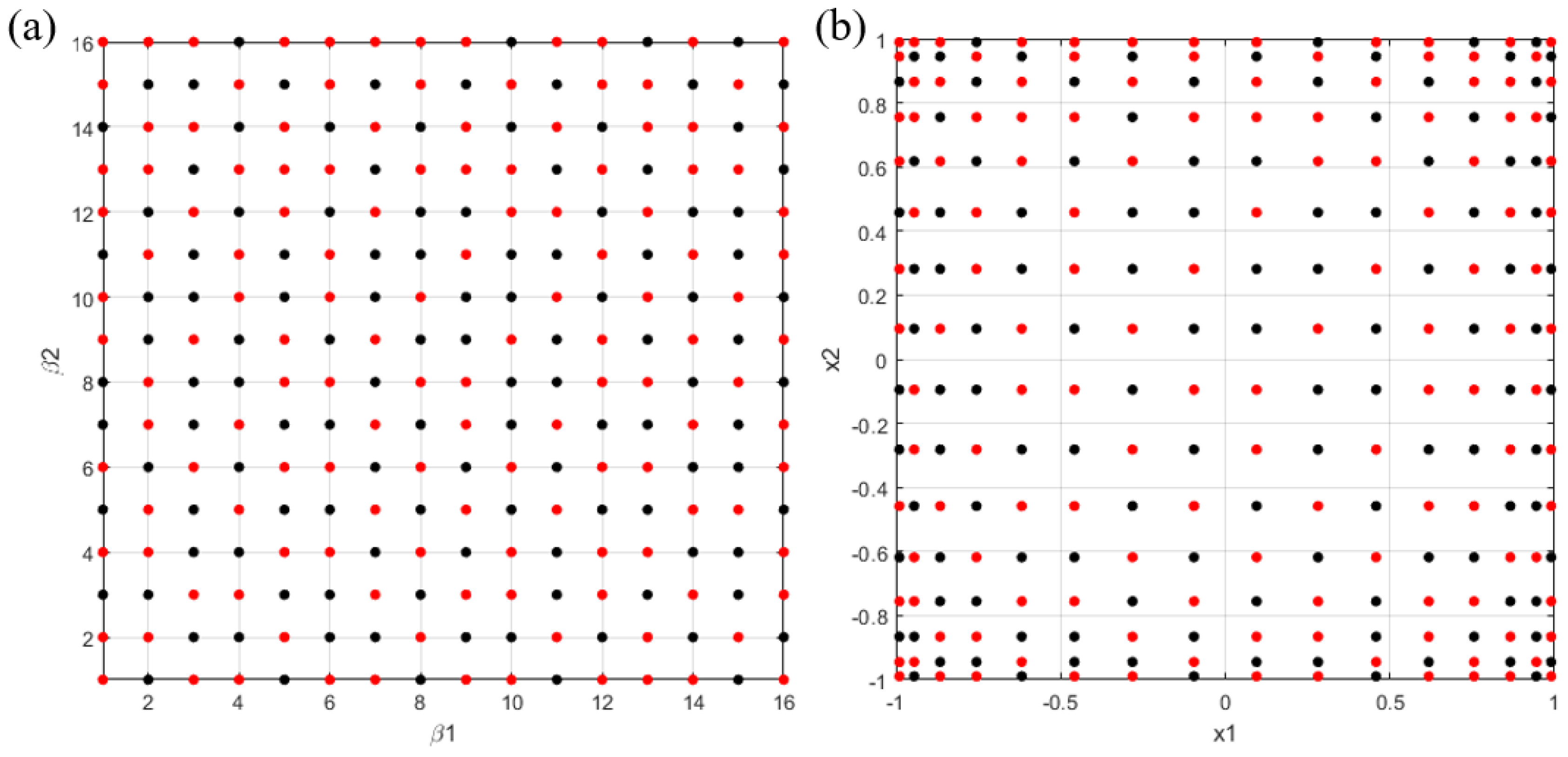
3.2.1. The Initial Candidate Samples

According to the theory of Gauss quadrature, when the Gauss points are utilized as a sample construction method to calculate the expansion coefficient of AOP, the AOP expansion can converge rapidly. Therefore, in this paper we will use the Gauss points as the candidate points. Before generating the Gauss points, it is essential to determine the weight function. According to Ref. [49], when the weight function, which is orthogonal to the polynomial basis, is consistent with the BPA of the evidence variable, the AOP expansion method can achieve an optimal accuracy. Therefore, the weight function is expressed as:
ω X i ( X i ) = r i n i δ j ( X i ) m ( x i ) x ¯ i x _ i ,
where x i is the i nd focal element of X i . x ¯ i and x _ i are the upper and lower bounds of x i .
When the weight function can be obtained by Equation (13), the Gauss points can be obtained as follows:
J n = [ a 0 b 1 b 1 a 1 b 2 b 2 a 2 a n 2 b n 1 b n 1 a n 1 ] .
where V T J n V = d i a g ( λ 1 , λ 2 , , λ n ) , V T V = I , and I is the n × n dimension identity matrix. The candidate points ε ^ i can be calculated by:
ε ^ i = λ i , i = 1 , 2 , .
In Equation (14), a k and b k of the AOP expansion can be expressed using by the theory of orthogonal polynomial [55,56] as:
a k = ε φ k ( ε ) , φ k ( ε ) φ k ( ε ) , φ k ( ε ) = 1 h k Ω ε φ k ( ε ) φ k ( ε ) ω ( ε ) , k = 0 , 1 , 2 , ,
b k = φ k ( ε ) , φ k ( ε ) φ k 1 ( ε ) , φ k 1 ( ε ) = 1 h k Ω φ k ( ε ) φ k ( ε ) ω ( ε ) , k = 1 , 2 , ,
where the coefficient b 0 is an arbitrary value and b 0 will be set as b 0 = ω ( x ) d x . , denotes the inner product with regard to a weight function in a specific domain Ω . ω ( ε ) is the weight function.
For the traditional AOP expansion method, the candidate points of the L -dimensional problems are the tensor product of Gauss integration points associated with the optimal Gauss weight function. The candidate points are expressed as:
ε = ε 1 × ε 2 × × ε L .
The total number of candidate points is:
N t o t a l = ( n 1 + 1 ) × ( n 2 + 1 ) × × ( n L + 1 ) .
The candidate points are obtained using Equation (15). In the following section, the process of selecting the sampling points from candidate points will be shown.

3.2.2. Space Uniformity Transformation for Candidate Points

The candidate points of the arbitrary orthogonal polynomial are Gauss integration points, which are denser along the boundary. For the sequential sampling scheme, the candidate points should satisfy the rule of being uniformly distributed. In other words, a candidate set of a sequential sampling scheme is symmetrical [57]. To overcome this limitation, a β space will be introduced to change the candidate points to an equal-weighted form. In β space, the coordinates of the integration points in ε set will be indicated by the component i ( i = 1 , 2 , , m ) , where m is the number of integration points for each variable. To illustrate the process of sequence sampling, an example showing the distribution of β space and ε set when k = 2 and m = 16 is shown in Figure 1. The selected sampling points from the candidate points are the red points.

3.2.3. The Sequence Sampling Process of Candidate Set

The performance of the final sample points will be influenced greatly by the selection of the initial sample points. Therefore, the initial sample points will be distributed uniformly in the candidate set space. Johnson et al. proposed a maximin metric measure [58]. Through this metric, whether the sampling candidate set is uniform or not can be evaluated. This method will rank the competing sample sets using the following scalar-valued criterion function [59]:
Φ q ( θ ) = ( i = 1 a 0 j = i + 1 a 0 d ( θ ( i ) , θ ( j ) ) q ) 1 / q .
q is set to 100 in this paper, which denotes a non-deterministic but relatively large positive integer. θ ( i ) is a sample set, a 0 indicates the number of candidate sample points, and the Euclidean distance d ( θ ( i ) , θ ( j ) ) can be expressed as
d ( θ ( j 1 ) , θ ( j 2 ) ) = ( i = 1 k | θ i ( j 1 ) θ i ( j 2 ) | p ) 1 / p ,
where θ i ( j 1 ) is the i nd variable of L-dimensional θ ( i ) , while p is the Euclidean norm and set as 2. In Equation (20), a smaller Φ q indicates that the sampling set is more uniform.
There are three steps in this sampling scheme. The first step is obtaining the initial sampling points of sequential sampling scheme. The number of the initial sample points is L × k L ( k denotes the number of Gauss integration points of each dimension and L denotes the number of dimension). In order to ensure the uniformity of the sample points, the initial row and the value of the first column will be set as a unique performance. The first row is set as 1 , 2 , , m , and the values of the first column are set as 1. In order to demonstrate the steps of the sequential sampling method, a case where k = 5 and L = 6 will be introduced. The initial matrix of sampling points is shown in Table 1.
The second step is minimizing the metric Φ q to calculate the rest elements in the initial sample set. The selected sample set is δ and the candidate set is denoted as θ . According to Ref. [60], the calculation of the smallest Φ q ( θ , θ 1 ( j ) ) can be simplified as
Φ q ( θ , θ 1 ( j ) ) = ( i = 1 a 0 d ( θ 0 ( i ) , θ 1 ( j ) ) q ) 1 / q ,
where θ 0 ( i ) δ are the old candidate samples and θ 0 ( j ) θ are new sampling points. The subscript 0 indicates the selected sampled set and the superscript ( i ) is the i th sample of θ . The subscript 1 indicates the candidate sampled set and the superscript ( j ) is the j th sample of δ .
Table 2 can demonstrate the process of selecting the rest of the samples from the candidate θ through minimizing Φ q . First of all, the calculation criterion Equation (22) is used to calculate the elements in the second column from second to sixth. Then, new selected samples are obtained from the candidate θ . The sampled space δ will be updated and the rest of the column elements can be obtained from 3 to m . The result is demonstrated in Table 2.
The final step of the sequence sampling is to calculate the rest values of the values. The rest c of columns can also be determined after the first m columns are calculated. In order to ensure that the samples in each dimension satisfy the uniformity rule, each dimension will be handled with a uniform method. Therefore, the first row is moved to the last, and the other rows move forward in sequence. Then, the second dimension row will be made uniform. The sequence sampling scheme can be repeated from column 6 to 10, as shown in Table 3.
After the initial candidate sampling scheme, the minimizing Φ q will be sustained to obtain the appropriate number of sampling points until the number of samples satisfies the value of N F in Equation (25).

3.2.4. Calculations of Expansion Coefficient

L -dimensional function Y ( ε ) can be approximated using the arbitrary polynomial expansion method as
Y ( ε ) = 0 i 1 + + i L n f i 1 , , i L φ j 1 , , j L ( ε ) .
According to the simplex format, the number of arbitrary polynomials basis and the expansion coefficient can be reduced from N t o t a l = ( n 1 + 1 ) × ( n 2 + 1 ) × × ( n L + 1 ) to a smaller value N s . N s is expressed as
N s = ( L + n ) ! L ! n ! .
As a result, in the same expansion order n i , the number of arbitrary polynomials is reduced to N s . The computational cost of expansion coefficients is reduced greatly, and the computational efficiency of AOP expansion will be improved.
In order to ensure the accuracy of the proposed SS-AOP method, the number of Gauss integration points N F which are used as the candidate points must be larger than that of expansion coefficients. In that case, the N F can be expressed as
N s ( L , n max ) = ( L + n max ) ! L ! n max ! < N F .
The least squares method can be used to calculate the expansion coefficients of AOP. Equation (23) can be transformed to the following formulation as
Y ( ε ) = 0 i 1 + + i L n f i 1 , , i L φ j 1 , , j L ( ε ) = β T α ,
β = [ β 1 β s ] T = [ f 0 , , 0 , , f i 1 , , i L ] T , 0 i 1 + + i L n ,
α = [ α 1 α s ] T = [ φ 0 , , 0 , , φ j 1 , , j L ] T , 0 i 1 + + i L n ,
In the three above equations, s is the number of expansion coefficients and the corresponding polynomial basis vector α . Through the least squares method, the expansion coefficients of SS-AOP can be calculated as
β = ( A T A ) 1 A T Y ,
Y indicates the original values for the response function, which are obtained through experiments or from current information. A is the assemble matrix which composed of the corresponding polynomial basis vector, which can be expressed as
A = [ α 1 ( ε 1 ) α s ( ε 1 ) α s ( ε s ) α 1 ( ε s ) ] ,
where s = N s and ε 1 , , ε s are the sampling points selected from the candidate points.

3.3. SS-AOP for the Response Analysis of Mechanics Property with Evidence Variables

Based on the SS-AOP shown in Equation (26), a global surrogate is established to deal with the response analysis of the mechanics property with evidence variables. The determined variables will be transformed to evidence variables. Considering the function y = f ( U ) , if a BPA structure of uncertain variables is obtained, the belief function ( B e l ) and plausibility function ( P l ) of the system can be represented by:
B e l ( y Y I ) = { u S k | y S k I = f ( u S k I ) Y I } m ( U s k I ) ,
P l ( y Y I ) = { u S k | y S k I = f ( u S k I ) Y I } m ( U s k I ) .
In the above equations, y S k I is the calculation result of the function on the joint focal element U S k I . The extreme value of y S k I can be calculated by the genetic optimization algorithm or the Monte Carlo simulation method. Additionally, the extreme value of y S k I can be expressed as:
y S k I = [ y S k _ , y S k ¯ ] = [ min Y ( U ) U U S k I , max Y ( U ) U U S k I ] ,
where y S k _ and y S k ¯ are the extreme value of the y S k I , respectively.
In engineering practice, the optimization design of structure or engineering systems with probability theory is always handled by cumulative probability. Similar to the probability theory, an interval consists of cumulative belief function and cumulative plausibility function, which can be defined as:
C B F ( Y ) = B e l ( y Y ) ,
C P F ( Y ) = P l ( y Y ) .
In the uncertainty analysis of evidence theory, calculating the mean value and variance is similar to the process used in probability theory. According to Ref. [43], both of these can be defined as follows:
μ ( y ) = S k = 1 N y S k I m ( U S k I ) ,
var ( y ) = S k = 1 N ( y S k I μ ( y ) ) 2 m ( U S k I ) .
Therefore, the statistics of y , such as the mean, variance value, and CBF and CPF, can be approximated using the SS-AOP method. These results will used for the uncertainty analysis conducted by the evidence theory model.

3.4. Procedure of SS-AOP for Uncertainty Analysis with Evidence Theory

This paper proposes a new method called the SS-AOP expansion method, which is introduced for the response analysis of a double-V NPR structure with evidence variables. The procedure of SS-AOP for auxetic structural dynamic analysis with evidence theory is shown in Figure 2.

4. Numerical Examples

In this section, several mathematical test functions and an engineering application for an auxetic structure with nonlinear large deformation are introduced to evaluate the effectiveness of the SS-AOP method. The traditional AOP expansion method [50] is introduced for comparison. In order to evaluate the computational accuracy of the different sampling methods, the Latin-hypercube-sampling-based arbitrary polynomial (LHS-AOP) expansion method and optimal-Latin-hypercube-sampling-based arbitrary polynomial (OLHS-AOP) expansion method are developed and then employed for comparison with the proposed SS-AOP method.

4.1. Mathematical Test Examples

The expressions of each mathematical function are given in Table 4 and feature nonlinear characteristics. According to Equation (25), the number of sampling points used to construct the SS-AOP method is set as 8, 17, 39, 77, 139, 231, and 363, respectively. The legend of these figures is expressed as ‘surrogate model-sampling method’. In order to demonstrate the effectiveness for the multidimensional case, the number of dimensions for each case is set to 4. To simplify the problem, these variables are independent. The range of each variable xi(i = 1,2,…4) is set as [ 1 , 1 ] .
A case where there are six focal elements is employed to demonstrate the effectiveness of the proposed SS-AOP method. The BPAs of each evidence variable are set as the same. Detailed information of uncertain variables is listed in Table 5.
Different from probability theory, the calculation result of the mean value and variance in evidence theory is given as an interval because the precise distribution of each focal element cannot be obtained; the given information for uncertain variables is several intervals and the probability of each interval. Therefore, the relative error of evidence theory is defined as the maximum relative error at the lower and upper boundary of the focal element, which are calculated by
μ m = max { | μ ¯ μ ¯ r e f μ ¯ r e f | , μ _ μ _ r e f μ _ r e f } , σ m = max { | σ ¯ σ ¯ r e f σ ¯ r e f | , σ _ σ _ r e f σ _ r e f } .
μ ¯ and μ _ denote the value of the lower and upper boundary of the mean value, σ ¯ and σ _ indicate the value of the lower and upper boundary of variance, and ( ) r e f is the reference solution.
The traditional AOP, SS-AOP, LHS-AOP, and OLHS-AOP methods are employed in this paper to obtain the results of the response analysis of the mathematical test functions. The calculation results for the relative error of the mean value and variance are shown in Figure 3, Figure 4, Figure 5 and Figure 6.
When compared to the traditional AOP method, the results from Figure 3, Figure 4, Figure 5 and Figure 6 show that the proposed SS-AOP method has a much higher accuracy than the traditional AOP method when the number of sampling points are the same. Moreover, the LHS-AOP and OLHS-AOP method can converge faster than the traditional AOP method. The main difference between the traditional AOP expansion approach and other methods in Figure 3 is that the expansion coefficient calculated by traditional AOP is the Gauss quadrature method, while the sampling technique is used in other methods. It indicates that, for uncertainty analysis by the evidence theory model, the convergence rate of the AOP expansion method with multiple variables can be greatly improved by using the sampling technique.
Based on a comparison with the LHS-AOP and OLHS-AOP method, the results from Figure 3, Figure 4, Figure 5 and Figure 6 show that the SS-AOP method can also achieve much higher results than LHS-AOP and OLHS-AOP. This is mainly because the sampling points of the LHS-AOP and OLHS-AOP methods are obtained by the approximately random sampling method, while the sampling points of the proposed SS-AOP method are selected by the sequence sampling scheme, and candidate points for sampling are generated using the Gauss points associated with the optimal Gauss weight function for each evidence variable. Therefore, for the uncertainty analysis of evidence theory, when the number of sampling points is the same, the accuracy of the SS-AOP method is much higher than the accuracy of the LHS-AOP and OLHS-AOP methods.

4.2. Engineering Application

In this section, a compression process with geometric nonlinearity and the large deformation of the popular double-V NPR structure is employed to verify the effectiveness of the proposed evidence-theory-based SS-AOP method. The normalized stiffness of the NPR structure is an important index used for analyzing the structural mechanics properties in large deformation under geometric nonlinearity. Additionally, the normalized stiffness of the double-V NPR structure is greatly affected by the error of the manufacturing technique and assembly approach used. The effectiveness of the analytical solution and the FE model of normalized stiffness of a double-V NPR microstructure is shown in Ref. [61]. The schematic model of a 2D double-V NPR microstructure is shown in Figure 7.
The ABAQUS software is used to simulate the large deformation and analyze the mechanical properties when the NPR structure in the compression process is geometrically nonlinear. The S-beam and L-beam are simulated as Euler–Bernoulli beams B23 because both of them are sufficiently slim. These beams are regarded as thin-walled structures and demonstrate the deformation modes of the NPR structure. Due to the constant displacement, lz = −5 mm will be set on the vertex A, and the large plastic deformation of double-V NPR is geometrically nonlinear. The compression process of the single unit cell in the z-direction is displayed in Figure 8. In this paper, due to structural symmetry, only half of the cell will be considered. The bottom node C is constrained in the z-direction. The vertex A is fixed in the x-direction and cannot rotate out of plane. The vertex B cannot rotate out of plane. These boundary conditions are equivalent to the periodic boundary condition. To illustrate the effectiveness of the mesh size, the convergence of the nonlinear analysis of double-V NPR structure is shown in Figure 9. When the mesh size is too large, the finite element simulation results will be unstable because the mesh is too large to describe the geometric features. In this paper, the double-V NPR structure was simulated when the mesh size converged.
In engineering applications, double-V NPR structures are usually processed with 3D-printing technology because of the structural complexity. In this paper, the material used for double-V NPR structures is ABS engineering plastics and the parameters of the basic material are: Young’s modulus E s = 2.2   GPa , Poisson’s ratio ν s = 0.39 , and mass density ρ s = 1.08   g / c m 3 . The normalized Young’s modulus of double-V NPR structures can be calculated by the relations Δ z = L z L z . Considering that the unpredictability of production processing can cause errors in the material’s parameter and structural size, such as Young’s modulus E s , the thickness of the L-beam T l , the angles θ 1 and θ 2 , and the length l are considered as the independent variables for evidence theory. The detailed distributions of BPAs are listed in Table 6.
The efficiency of the proposed SS-AOP expansion method is evaluated based on the total execution time. The final execution times taken by the traditional AOP, SS-AOP, LHS-AOP, and OLHS-AOP methods to calculate the normalized Young’s modulus with large deformation are listed in Table 7.
From Table 7, the computational result shows that with regard to the execution time of SS-AOP, LHS-AOPs and OLHS-AOP can achieve a much higher computational efficiency than the traditional AOP method. Meanwhile, the execution time of the proposed SS-AOP method is very close to that of the LHS-AOP and OLHS-AOP methods, as the sampling points of the proposed SS-AOP, LHS-AOP, and OLHS-AOP method are the same.
The CBF and CPF of complex structural-response analyses can be used as effective guidance for structure design and reliability-based optimization in the evidence theory model. The CBF and CPF of the normalized Young’s modulus of the double-V NPR structure model are calculated using the proposed SS-AOP method, the LHS-AOP method, and the OLHS-AOP method at the same sampling points, where the number of sampling points is 23. The reference solution is the traditional AOP with a retained expansion order of 6 for each evidence variable. The results obtained for CBF and CPF are plotted in Figure 10.
The results plotted in Figure 9 show that the CBF and CPF obtained through SS-AOP almost coincide with the reference solutions. This indicates that the proposed SS-AOP method has a good accuracy. For comparison, the calculation results of the LHS-AOP method and OLHS-AOP method were different from those of the reference solutions. Thus, the execution times for the SS-AOP, LHS-AOP, and OLHS-AOP are almost the same, as displayed in Table 7. This indicates that, with a similar execution time, the accuracy of the SS-AOP method is much higher than that of LHS-AOP method and the OLHS-AOP method without scarifying the efficiency.

5. Conclusions

In engineering practice, epistemic uncertainties usually exist in complex auxetic structures. These uncertainties can cause great changes in the mechanical properties of structures. In this paper, the uncertain variables are modelled using the evidence theory model. For the response analysis of the auxetic structural mechanics properties with the evidence variables, a new SS-AOP method under evidence theory is proposed. In SS-AOP, a sequential-sampling technique is introduced to calculate the expansion coefficients, and the sampling points used for calculating the expansion coefficient can be reduced effectively. In order to demonstrate the effectiveness of the proposed SS-AOP method, the LHS-AOP and OLHS-AOP methods were also developed for comparison. In LHS-AOP and OLHS-AOP, the expansion coefficient of AOP expansion is calculated using the Latin hypercube sampling scheme and the optimal Latin hypercube sampling scheme, respectively.
Four mathematical test functions with nonlinear characteristics and an engineering application of the mechanics properties response analysis for a double-V NPR structure were introduced to demonstrate the effectiveness of the proposed SS-AOP method. The proposed SS-AOP method was compared with the traditional AOP, the LHS-AOP method, and the OLHS-AOP method. The main conclusions are as follows:
(1)
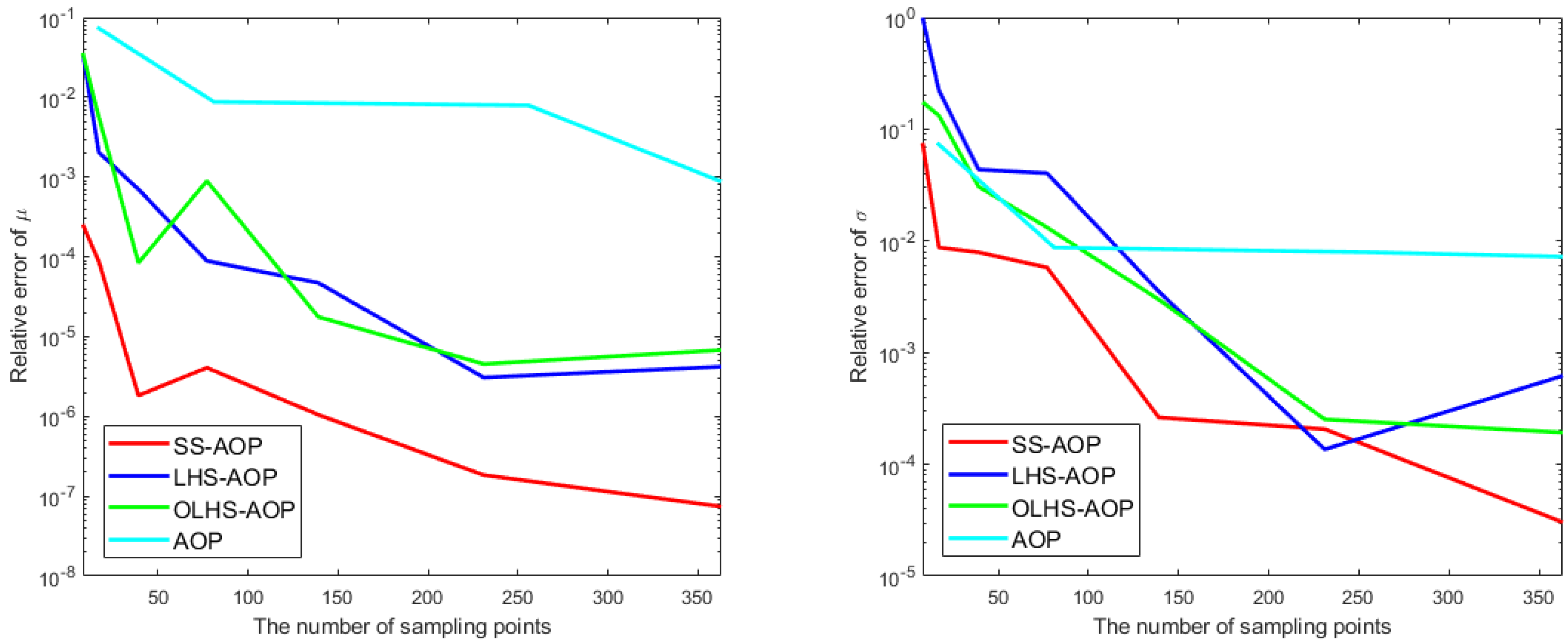
The computational efficiency of the proposed SS-AOP method is much higher than that of the traditional AOP method without sacrificing any accuracy. This is because the number of the polynomial basis of SS-AOP is reduced by using the simplex format, while the sequential-sampling technique is introduced to reduce number of the sampling points which are used to calculate the expansion coefficients.
(2)
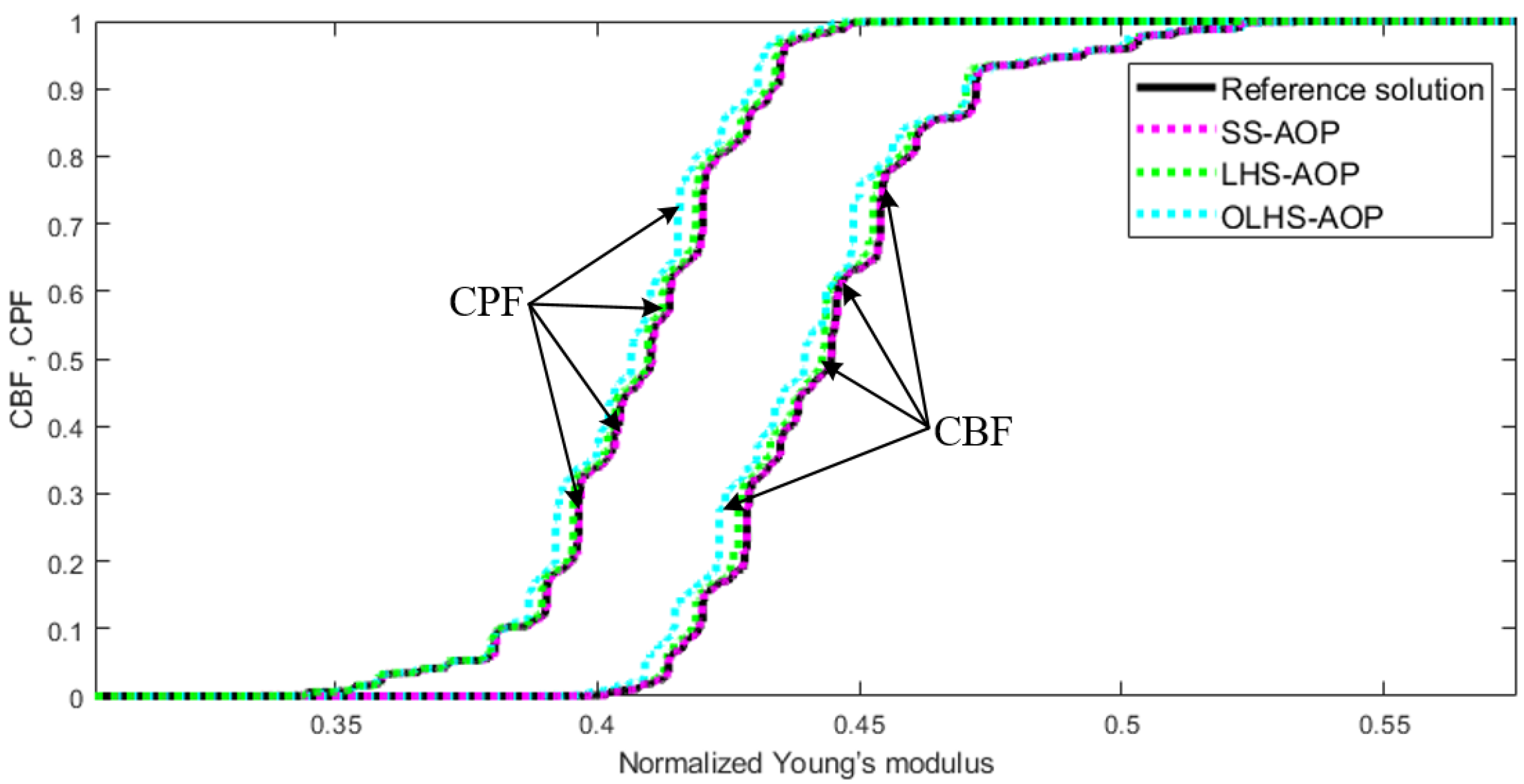
In comparison to the LHS-AOP and OLHS-AOP methods, the proposed SS-AOP method can achieve a higher accuracy. This is because, in the SS-AOP method, the sequence sampling scheme can select sampling points uniformly from candidate points. In particular, the candidate points used for sampling are generated using the Gauss points associated with the optimal Gauss weight function for each evidence variable. In comparison, the sampling points of the LHS-AOP method and the OLHS-AOP method are fairly random.
As a conclusion, the proposed evidence-theory-based SS-AOP method provides a more efficient tool for the epistemic uncertainty analysis of evidence theory. The computational efficiency of the proposed SS-AOP method is better than that of the conventional evidence-theory-based AOP methods and the Latin-hypercube-sampling-based orthogonal polynomial expansion methods. In an appropriate application, the proposed SS-AOP method may be applied to other engineering scenarios with uncertain parameters, such as the dynamic analysis of crashworthy thin-walled structures and strong nonlinear problems. Despite this, the proposed SS-AOP method can reduce the computational cost for epistemic uncertainty analysis based on the evidence theory model. For the epistemic uncertainty analysis of evidence theory, the extreme analysis of each focal element is an important step. The traditional method of extreme analysis is carried out using the genetic algorithm to calculate the maximum value. For multidimensional problems, with the increase in the number of focal elements, the number of joint focal elements becomes very large, leading to a huge computational burden. The question of how to effectively and accurately obtain the maximum value of each joint focal element needs to be studied further.

Author Contributions

Conceptualization, Q.G. and S.Y.; methodology, S.Y.; software, H.Q.; validation, H.Q.; formal analysis, H.Q.; investigation, Q.G. and S.Y.; resources, Q.G. and S.Y.; data curation, H.Q.; writing—original draft preparation, H.Q.; writing—review and editing, Q.G. and S.Y.; visualization, H.Q.; supervision, S.Y.; project administration, S.Y.; funding acquisition, S.Y. All authors have read and agreed to the published version of the manuscript.

Funding

The paper is supported Natural Science Foundation of Hunan Province, China (No.2020JJ5686).

Acknowledgments

The author would like to sincerely thank Yin and Gao for their kind guidance.

Conflicts of Interest

We declare that we have no financial and personal relationships with other people or organizations that can inappropriately influence our work, there is no professional or other personal interest of any nature or kind in any product, service and/or company that could be construed as influencing the position presented in, or the review of, the manuscript entitled “An Efficient Orthogonal Polynomial Method for Auxetic Structure Analysis with Epistemic Uncertainties”.

References

  1. Gao, Q.; Liao, W.H. Energy absorption of thin-walled tube filled with gradient auxetic structures—Theory and simulation. Int. J. Mech. Sci. 2021, 201, 106475. [Google Scholar] [CrossRef]
  2. Wang, K.; Liu, Y.; Wang, J.; Xiang, J.; Yao, S.; Peng, Y. On crashworthiness behaviors of 3D printed multi-cell filled thin-walled structures. Eng. Struct. 2022, 254, 113907. [Google Scholar] [CrossRef]
  3. Xu, X.; Xu, G.; Chen, J.; Liu, Z.; Chen, X.; Zhang, Y.; Fang, J.; Gao, Y. Multi-objective design optimization using hybrid search algorithms with interval uncertainty for thin-walled structures. Thin-Walled Struct. 2022, 175, 109218. [Google Scholar] [CrossRef]
  4. Yang, W.; Huang, R.; Liu, J.; Liu, J.; Huang, W. Ballistic impact responses and failure mechanism of composite double-arrow auxetic structure. Thin-Walled Struct. 2022, 174, 109087. [Google Scholar] [CrossRef]
  5. Zhu, Y.; Jiang, S.; Poh, L.H.; Shao, Y.; Wang, Q. Enhanced hexa-missing rib auxetics for achieving targeted constant NPR and in-plane isotropy at finite deformation. Smart Mater. Struct. 2020, 29, 045030. [Google Scholar] [CrossRef]
  6. Zhu, Y.; Wang, Z.; Poh., L.H. Auxetic hexachiral structures with wavy ligaments for large elasto-plastic deformation. Smart Mater. Struct. 2018, 27, 055001. [Google Scholar] [CrossRef]
  7. Zhu, Y.; Zeng, Z.; Wang, Z.P.; Poh, L.H.; Shao, Y. Hierarchical hexachiral auxetics for large elasto-plastic deformation. Mater. Res. Express 2019, 6, 085701. [Google Scholar] [CrossRef]
  8. Zhu, Y.; Jiang, S.; Li, J.; Pokkalla, D.K.; Wang, Q.; Zhang, C. Novel Isotropic Anti-Tri-Missing Rib Auxetics with Prescribed In-Plane Mechanical Properties Over Large Deformations. Int. J. Appl. Mech. 2021, 13, 2150115. [Google Scholar] [CrossRef]
  9. Nayak, S.; Chakraverty, S. Non-probabilistic approach to investigate uncertain conjugate heat transfer in an imprecisely defined plate. Int. J. Heat Mass Transf. 2013, 67, 445–454. [Google Scholar] [CrossRef]
  10. Wang, C.; Qiu, Z.; Xu, M.; Li, Y. Novel reliability-based optimization method for thermal structure with hybrid random, interval and fuzzy parameters. Appl. Math. Model. 2017, 47, 573–586. [Google Scholar] [CrossRef]
  11. Chowdhury, R.; Rao, B.N. Hybrid High Dimensional Model Representation for reliability analysis. Comput. Methods Appl. Mech. Eng. 2009, 198, 753–765. [Google Scholar] [CrossRef]
  12. Choi, K.K.; Youn, B.D.; Yang, R.J. Moving least square method for reliability-based design optimization. In Proceedings of the 4th World Congress of Structural and Multidisciplinary Optimization, Dalian, China, 4–8 June 2001; pp. 1–6. [Google Scholar]
  13. Youn, B.D.; Choi, K.K. A New Response Surface Methodology for Reliability Based Design Optimization. Comput. Struct. 2004, 82, 241–256. [Google Scholar] [CrossRef]
  14. Paz, J.; Díaz, J.; Romera, L. Analytical and numerical crashworthiness uncertainty quantification of metallic thin-walled energy absorbers. Thin-Walled Struct. 2020, 157, 107022. [Google Scholar] [CrossRef]
  15. Qiu, N.; Gao, Y.; Fang, J.; Sun, G.; Li, Q.; Kim, N.H. Crashworthiness optimization with uncertainty from surrogate model and numerical error. Thin-Walled Struct. 2018, 129, 457–472. [Google Scholar] [CrossRef]
  16. Li, F.; Sun, G.; Huang, X.; Rong, J.; Li, Q. Multiobjective robust optimization for crashworthiness design of foam filled thin-walled structures with random and interval uncertainties. Eng. Struct. 2015, 88, 111–124. [Google Scholar] [CrossRef]
  17. Zhang, Y.; Xu, X.; Sun, G.; Lai, X.; Li, Q. Nondeterministic optimization of tapered sandwich column for crashworthiness. Thin-Walled Struct. 2018, 122, 193–207. [Google Scholar] [CrossRef]
  18. Olalusi, O.B.; Spyridis, P. Uncertainty modelling and analysis of the concrete edge breakout resistance of single anchors in shear. Eng. Struct. 2020, 222, 111112. [Google Scholar] [CrossRef]
  19. Su, L.; Li, X.-L.; Jiang, Y.-P. Comparison of methodologies for seismic fragility analysis of unreinforced masonry buildings considering epistemic uncertainty. Eng. Struct. 2020, 205, 110059. [Google Scholar] [CrossRef]
  20. Yang, Y.; Peng, J.; Liu, X.; Cai, S.C.; Zhang, J. Probability analysis of web cracking of corroded prestressed concrete box-girder bridges considering aleatory and epistemic uncertainties. Eng. Struct. 2021, 228, 111486. [Google Scholar] [CrossRef]
  21. Ni, P.; Li, J.; Hao, H.; Xia, Y.; Du, X. Stochastic dynamic analysis of marine risers considering fluid-structure interaction and system uncertainties. Eng. Struct. 2019, 19, 109507. [Google Scholar] [CrossRef]
  22. Hoffman, F.O.; Hammonds, J.S. Propagation of uncertainty in risk assessments: The need to distinguish between uncertainty due to lack of knowledge and uncertainty due to variability. Risk Anal. 1994, 14, 707–712. [Google Scholar] [CrossRef] [PubMed]
  23. Rao, K.D.; Kushwaha, H.; Verma, A.K.; Srividya, A. Quantification of epistemic and aleatory uncertainties in level-1 probabilistic safety assessment studies. Reliab. Eng. Syst. Saf. 2007, 92, 947–956. [Google Scholar]
  24. Elishakoff, I.; Elisseeff, P.; Glegg, S. Non-probabilistic convex-theoretic modeling of scatter in material properties. AIAA J. 1994, 32, 843–849. [Google Scholar] [CrossRef]
  25. Zadeh, L. Fuzzy sets. Inf. Control 1965, 8, 338–353. [Google Scholar] [CrossRef] [Green Version]
  26. Ben-Haim, Y.; Elishakoff, I. Convex Models of Uncertainty in Applied Mechanics; Elsevier: Amsterdam, The Netherlands, 1990. [Google Scholar]
  27. Jiang, C.; Han, X.; Lu, G.Y.; Liu, J.; Zhang, Z.; Bai, Y.C. Correlation analysis of non-probabilistic convex model and corresponding structural reliability technique. Comput. Methods Appl. Mech. Eng. 2011, 200, 2528–2546. [Google Scholar] [CrossRef]
  28. Kang, Z.; Zhang, W. Construction and application of an ellipsoidal convex model using a semi-definite programming formulation from measured data. Comput. Methods Appl. Mech. Eng. 2016, 300, 461–489. [Google Scholar] [CrossRef]
  29. Qiu, Z.; Elishakoff, I. Antioptimization of structures with large uncertain-but-non-random parameters via interval analysis. Comput. Methods Appl. Mech. Eng. 1998, 152, 361–372. [Google Scholar] [CrossRef]
  30. Yager, R.; Fedrizzi, M.; Kacprzyk, J. Advances in the Dempster-Shafer Theory of Evidence; John Wiley & Sons: New York, NY, USA, 1994. [Google Scholar]
  31. Yang, J.; Huang, H.Z.; He, L.P.; Zhu, S.P.; Wen, D. Risk evaluation in failure mode and effects analysis of aircraft turbine rotor blades using Dempster-Shafer evidence theory under uncertainty. Eng. Fail. Anal. 2011, 18, 2084–2092. [Google Scholar] [CrossRef]
  32. Helton, J.C.; Johnson, J.D. Quantification of margins and uncertainties: Alternative representations of epistemic uncertainty. Reliab. Eng. Syst. Saf. 2011, 96, 1034–1052. [Google Scholar] [CrossRef]
  33. Oberkampf, W.L.; Helton, J.C. Investigation of evidence theory for engineering applications. In Proceedings of the AIAA 2002–1569, 4th Non-Deterministic Approaches Forum, Denver, CO, USA, 22–25 April 2002. [Google Scholar]
  34. Klir, G.J.; Smith, R.M. On measuring uncertainty and uncertainty-based information: Recent developments. Ann. Math. Artif. Intell. 2001, 32, 5–33. [Google Scholar] [CrossRef]
  35. Bai, Y.C.; Han, X.; Jiang, C.; Liu, J. Comparative study of metamodeling techniques for reliability analysis using evidence theory. Adv. Eng. Softw. 2012, 53, 61–71. [Google Scholar] [CrossRef]
  36. Zhang, Z.; Jiang, C.; Han, X.; Hu, D.; Yu, S. A response surface approach for structural reliability analysis using evidence theory. Adv. Eng. Softw. 2014, 69, 37–45. [Google Scholar] [CrossRef]
  37. Xiao, M.; Gao, L.; Xiong, H.; Luo, Z. An efficient method for reliability analysis under epistemic uncertainty based on evidence theory and support vector regression. Taylor Fr. 2015, 26, 340–364. [Google Scholar] [CrossRef]
  38. Cao, L.; Liu, J.; Wang, Q.; Jiang, C.; Zhang, L. An efficient structural uncertainty propagation method based on evidence domain analysis. Eng. Struct. 2019, 194, 26–35. [Google Scholar] [CrossRef]
  39. Bai, Y.C.; Jiang, C.; Han, X.; Hu, D.A. Evidence-theory-based structural static and dynamic response analysis under epistemic uncertainties. Finite Elem. Anal. Des. 2013, 68, 52–62. [Google Scholar] [CrossRef]
  40. Yin, S.; Yu, D.; Yin, H.; Lü, H.; Xia, B. Hybrid evidence theory-based finite element/statistical energy analysis method for mid-frequency analysis of built-up systems with epistemic uncertainties. Mech. Syst. Signal Process. 2017, 93, 204–224. [Google Scholar] [CrossRef]
  41. Chen, N.; Yu, D.; Xia, B. Evidence-theory-based analysis for the prediction of exterior acoustic field with epistemic uncertainties. Eng. Anal. Bound. Elem. 2015, 50, 402–411. [Google Scholar] [CrossRef]
  42. Helton, J.C.; Johnson, J.D.; Oberkampf, W.L.; Storlie, C.B. A sampling-based computational strategy for the representation of epistemic uncertainty in model predictions with evidence theory. Comput. Methods Appl. Mech. Eng. 2007, 196, 3980–3998. [Google Scholar] [CrossRef] [Green Version]
  43. Jiang, C.; Zhang, Z.; Han, X.; Liu, J. A novel evidence-theory-based reliability analysis method for structures with epistemic uncertainty. Comput. Struct. 2013, 129, 1–12. [Google Scholar] [CrossRef]
  44. Eldred, M.S.; Swiler, L.P.; Tang, G. Mixed aleatory-epistemic uncertainty quantification with stochastic expansions and optimization-based interval estimation. Reliab. Eng. Syst. Saf. 2011, 96, 1092–1113. [Google Scholar] [CrossRef]
  45. Yin, S.; Yu, D.; Yin, H.; Xia, B. A new evidence-theory-based method for response analysis of acoustic system with epistemic uncertainty by using Jacobi expansion. Comput. Meth. Appl. Mech. Eng. 2017, 322, 419–440. [Google Scholar] [CrossRef]
  46. Chen, N.; Hu, Y.; Yu, D.; Liu, J.; Beer, M. A polynomial expansion approach for response analysis of periodical composite structural-acoustic problems with multi-scale mixed aleatory and epistemic uncertainties. Comput. Methods Appl. Mech. Eng. 2018, 342, 509–531. [Google Scholar] [CrossRef]
  47. Chen, N.; Xia, S.; Yu, D.; Liu, J.; Beer, M. Hybrid interval and random analysis for structural-acoustic systems including periodical composites and multi-scale bounded hybrid uncertain parameters. Mech. Syst. Sig. Process. 2019, 115, 524–544. [Google Scholar] [CrossRef]
  48. Wang, C. Evidence-theory-based uncertain parameter identification method for mechanical systems with imprecise information. Comput. Methods Appl. Mech. Eng. 2019, 351, 281–296. [Google Scholar] [CrossRef]
  49. Yin, S.; Yu, D.; Luo, Z.; Xia, B. An arbitrary polynomial chaos expansion approach for response analysis of acoustic systems with epistemic uncertainty. Comput. Methods Appl. Mech. Eng. 2018, 332, 280–302. [Google Scholar] [CrossRef]
  50. Yin, S.; Yu, D.; Luo, Z.; Xia, B. Unified polynomial expansion for interval and random response analysis of uncertain structure–acoustic system with arbitrary probability distribution. Comput. Methods Appl. Mech. Eng. 2018, 336, 260–285. [Google Scholar] [CrossRef]
  51. Gorissen, D.; Couckuyt, I.; Demeester, P.; Dhaene, T.; Crombecq, K. A surrogate modeling and adaptive sampling toolbox for computer based design. J. Mach. Learn. Res. 2010, 11, 2051–2055. [Google Scholar]
  52. Romero, V.J.; Swiler, L.P.; Giunta, A.A. Construction of response surfaces based on progressive-lattice-sampling experimental designs with application to uncertainty propagation. Struct. Saf. 2004, 26, 201–219. [Google Scholar] [CrossRef]
  53. Bae, H.R.; Grandhi, R.V.; Canfield, R.A. Epistemic uncertainty quantification techniques including evidence theory for large-scale structures. Comput. Struct. 2004, 82, 1101–1112. [Google Scholar] [CrossRef]
  54. Gautschi, W. Orthogonal Polynomials: Computation and Approximation; Oxford University Press: Oxford, UK, 2004. [Google Scholar]
  55. Chen, N.; Yu, D.; Xia, B. Hybrid uncertain analysis for the prediction of exterior acoustic field with interval and random parameters. Comput. Struct. 2014, 141, 9–18. [Google Scholar] [CrossRef]
  56. Chen, J.; Xia, B.; Liu, J. A sparse polynomial surrogate model for phononic crystals with uncertain parameters. Comput. Methods Appl. Mech. Eng. 2018, 339, 681–703. [Google Scholar] [CrossRef]
  57. Oladyshkin, S.; Nowak, W. Data-driven uncertainty quantification using the arbitrary polynomial chaos expansion. Reliab. Eng. Syst. Saf. 2012, 106, 179–190. [Google Scholar] [CrossRef]
  58. Johnson, M.E.; Moore, L.M.; Ylvisaker, D. Minimax and maximin distance designs. J. Statist. Plann. Inference 1990, 26, 131–148. [Google Scholar] [CrossRef]
  59. Morris, M.D.; Mitchell, T.J. Exploratory designs for computational experiments. J. Statist. Plann. Inference 1992, 43, 381–402. [Google Scholar] [CrossRef] [Green Version]
  60. Wu, J.; Luo, Z.; Zheng, J.; Jiang, C. Incremental modeling of a new high-order polynomial surrogate model. Appl. Math. Model. 2016, 40, 4681–4699. [Google Scholar] [CrossRef]
  61. Gao, Q.; Tan, C.A.; Hulbert, G.; Wang, L. Geometrically nonlinear mechanical properties of auxetic double-V microstructures with negative Poisson’s ratio. Eur. J. Mech. A Solids 2020, 80, 103933. [Google Scholar] [CrossRef]
Figure 1. (a) Candidate points in β space; (b) candidate points in ε set.
Mca 27 00049 g001
Figure 2. Flow chart of the proposed SS-AOP for the evidence theory model.
Mca 27 00049 g002
Figure 3. The relative error of mean value and variance for Case 1.
Mca 27 00049 g003
Figure 4. The relative error of mean value and variance for Case 2.
Mca 27 00049 g004
Figure 5. The relative error of mean value and variance for Case 3.
Mca 27 00049 g005
Figure 6. The relative error of mean value and variance for Case 4.
Mca 27 00049 g006
Figure 7. Schematic model of a 2D double-V NPR microstructure.
Mca 27 00049 g007
Figure 8. The deformation process of half a unit cell.
Mca 27 00049 g008
Figure 9. The convergence of the mesh size of a 2D double-V NPR microstructure.
Mca 27 00049 g009
Figure 10. The CBF and CPF of the double-V NPR structure responses obtained with 5 focal elements for different methods.
Mca 27 00049 g010
Table 1. The initialization design matrix of position for k = 5 and L = 6 .
DimensionNo. of Samples
12345630
112345
21
31
41
51
61
Table 2. The design matrix of position for k = 5 and L = 6 .
DimensionNo. of Samples
12345630
112345
215151
315154
415315
515513
615531
Table 3. The first design matrix of position for k = 5 and L = 6 .
DimensionNo. of Samples
1234567891030
21515112345
315154
415315
515513
615531
112345
Table 4. Mathematical test functions.
FunctionsExpressionDomainDimension
Case 1 y = i = 1 4 arctan ( x i + i ) 1 x i 1 4
Case 2 y = i = 1 4 exp ( x i + i ) 1 x i 1 4
Case 3 y = i = 1 4 sin ( x i + i ) 1 x i 1 4
Case 4 y = i = 1 4 cos ( x i + i ) 1 x i 1 4
Table 5. BPA of the evidence variable for the case.
IntervalBPA (%)
[−1, −0.3]0.1
[−0.3, −0.1]5
[−0.1, 0]44.9
[0, 0.1]44.9
[0.1, 0.3]5
[0.3, 1]0.1
Table 6. The BPAs of an NPR structure with 5 elements.
T l   BPA
(%)
θ 1   BPA
(%)
θ 2   BPA
(%)
l BPA
(%)
E s   BPA
(%)
Interval
(mm)
Interval
(°)
Interval
(°)
Interval
(mm)
Interval
(MPa)
[0.99, 0.995]7[57, 59.1]0.1[28.5, 29.55]0.1[28.8, 29.64]6[2090, 2167]12
[0.995, 0.998]15[59.1, 59.7]6[29.55, 29.85]6[29.64, 29.88]42[2167, 2189]18
[0.998, 1.002]51[59.7, 60.03]88.7[29.85, 30.15]88.7[29.88, 30.12]5[2189, 2211]38
[1.002, 1.005]18[60.03, 60.9]5[30.15, 30.45]5[30.12, 30.36]42[2211, 2233]12
[1.005, 1.01]9[60.9, 63]0.2[30.45, 31.5]0.2[30.36, 31.2]5[2233, 2310]20
Table 7. Execution time of different methods for the response analysis of double-V NPR structures.
MethodTraditional AOPSS-AOPLHS-AOPOLHS-AOP
Execution time337,821.7 s464.1 s463.5 s464.3 s
Publisher’s Note: MDPI stays neutral with regard to jurisdictional claims in published maps and institutional affiliations.

