
Reduced Order Modeling Using Advection-Aware Autoencoders


Abstract
:1. Introduction
2. Related Work
3. Methodology
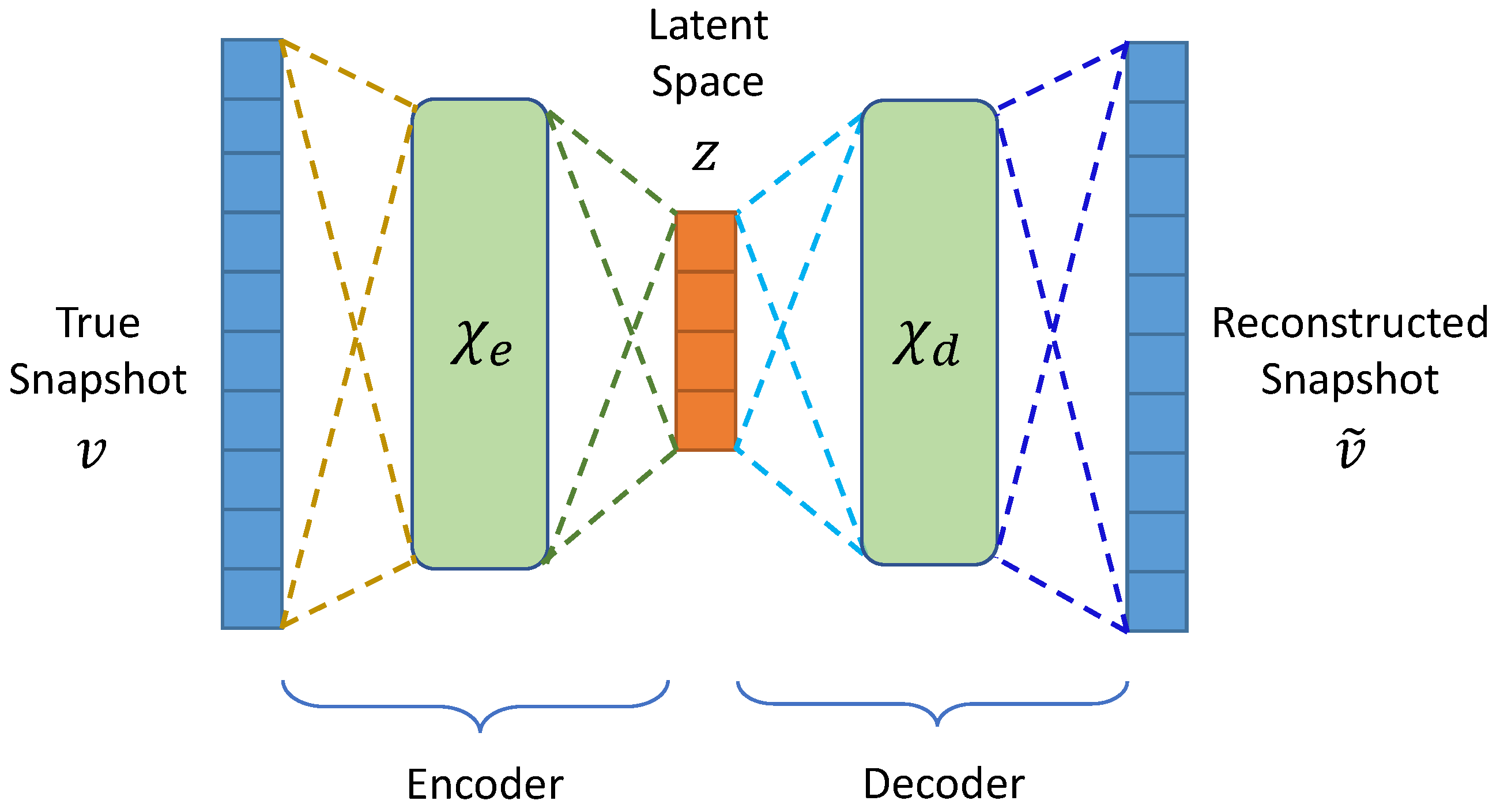
3.1. Autoencoders
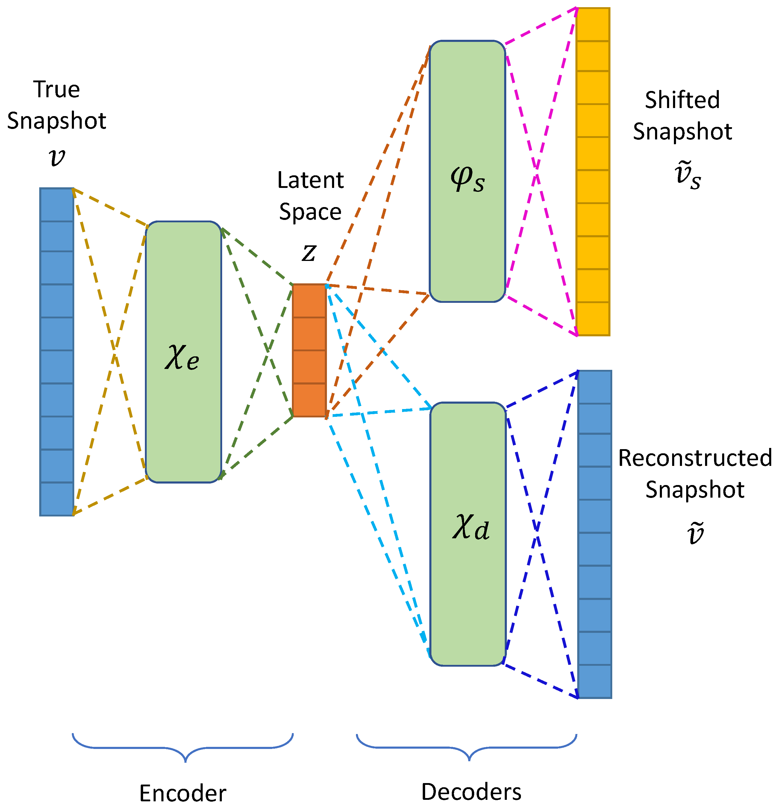
3.2. Advection-Aware Autoencoder Design
3.3. Long-Short-Term Memory (LSTM) Network
4. Results
4.1. Linear Advection Problem
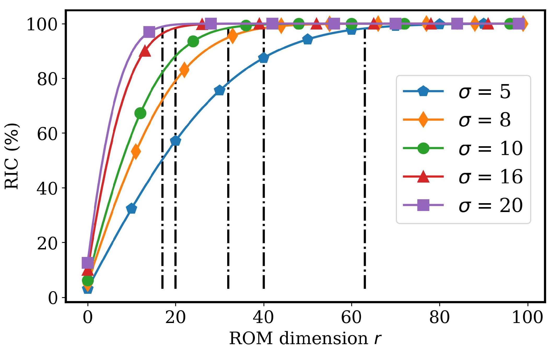
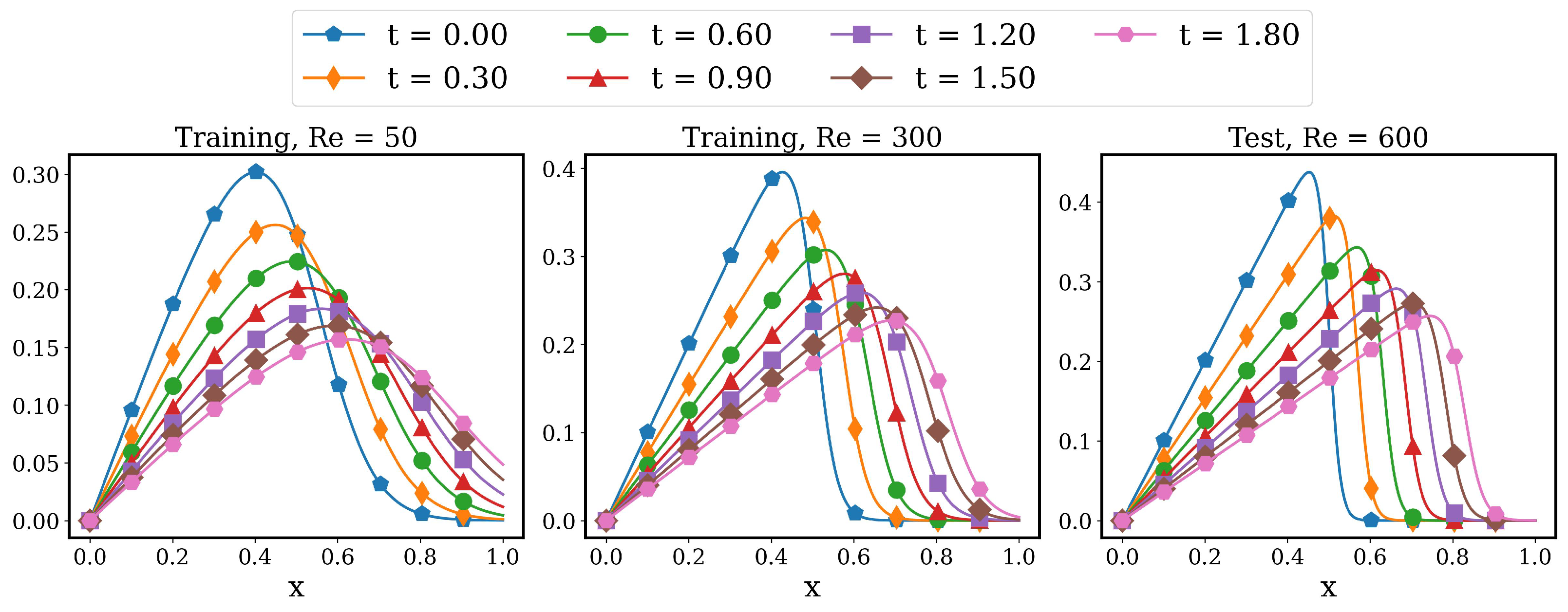
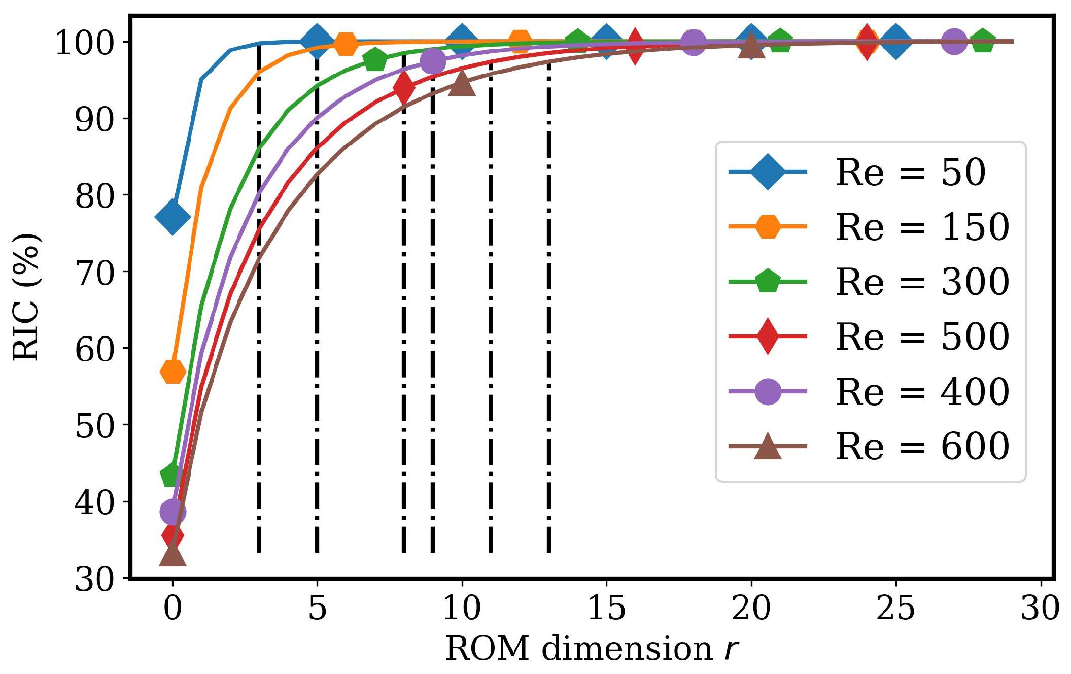
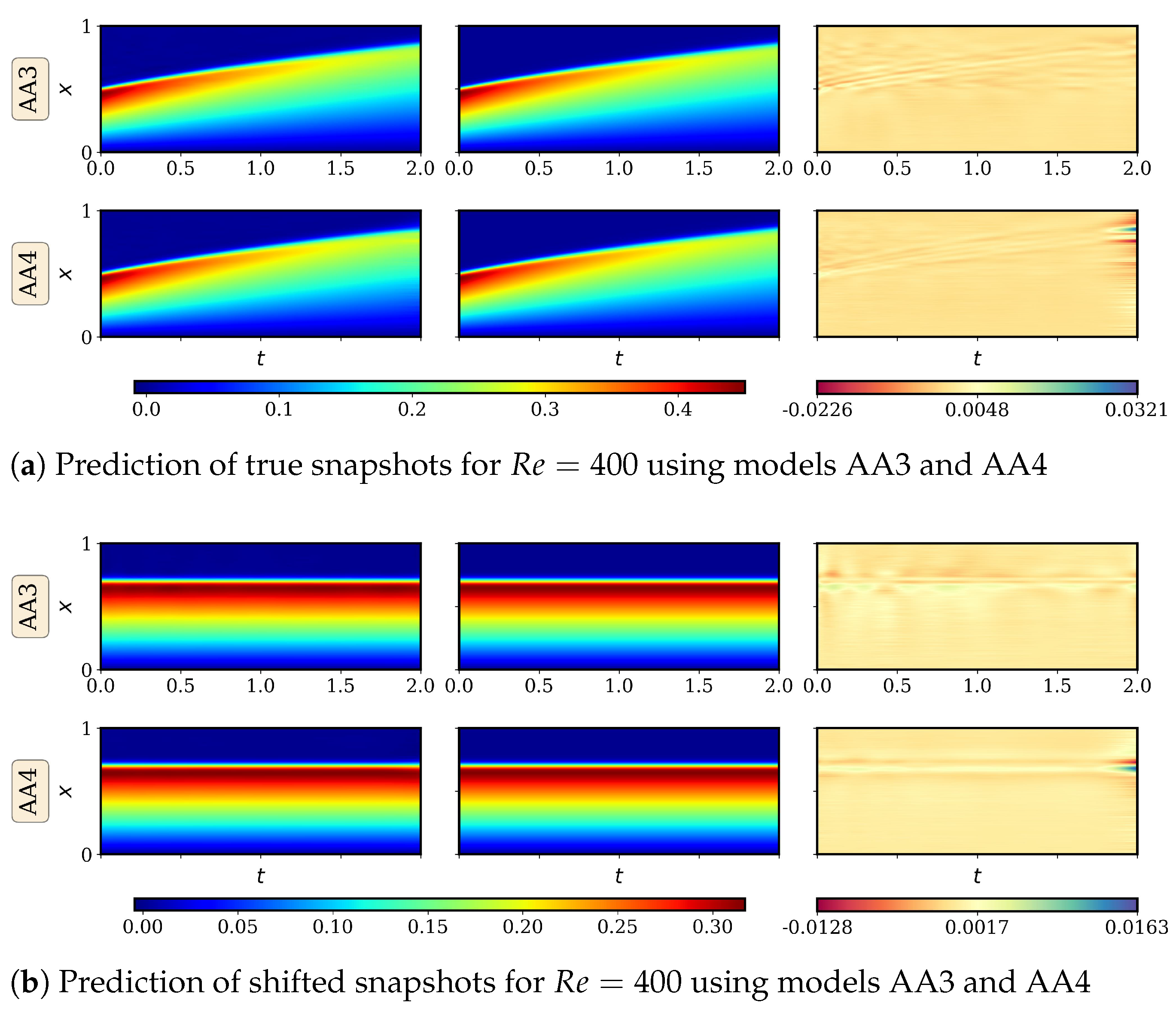
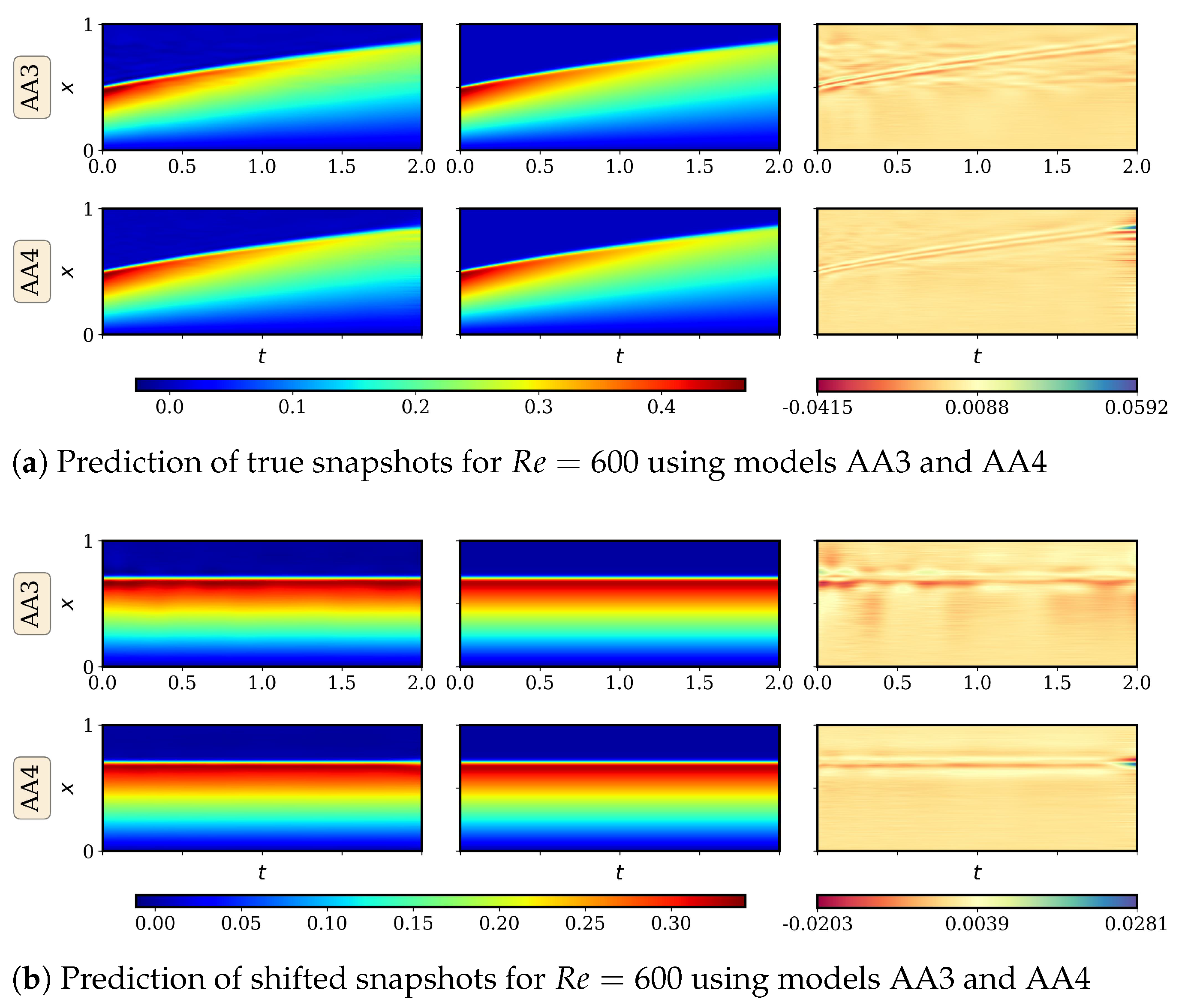
4.2. Advecting Viscous Shock Problem
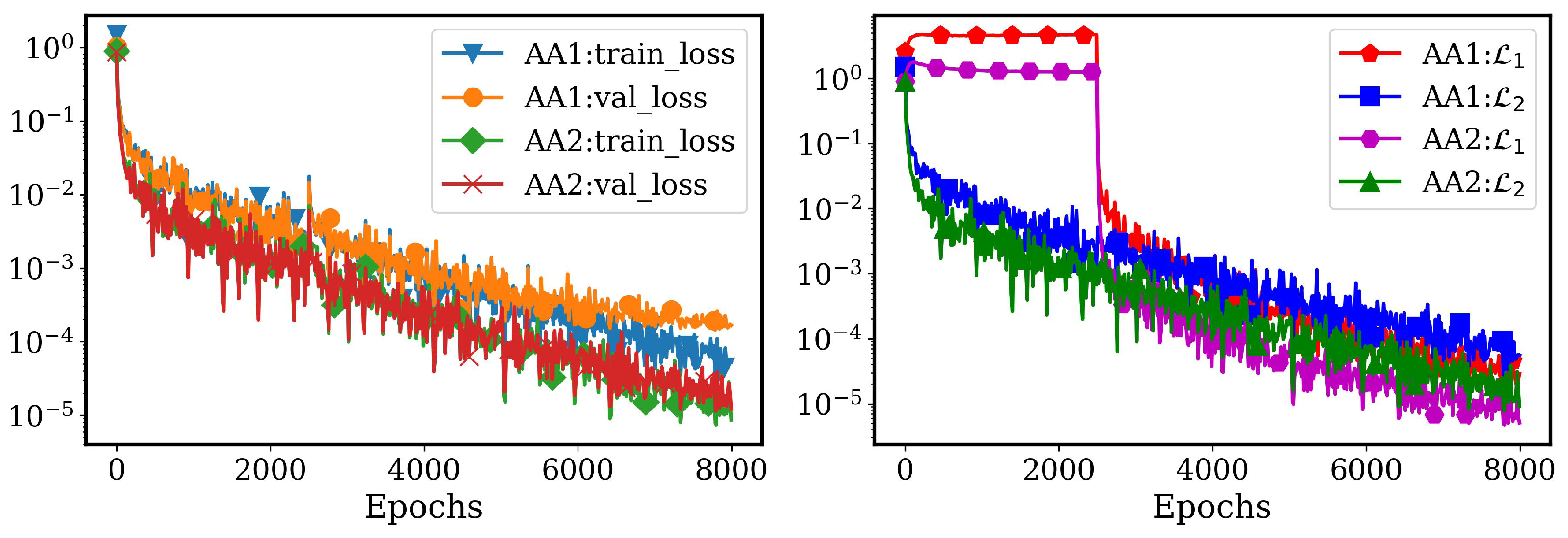
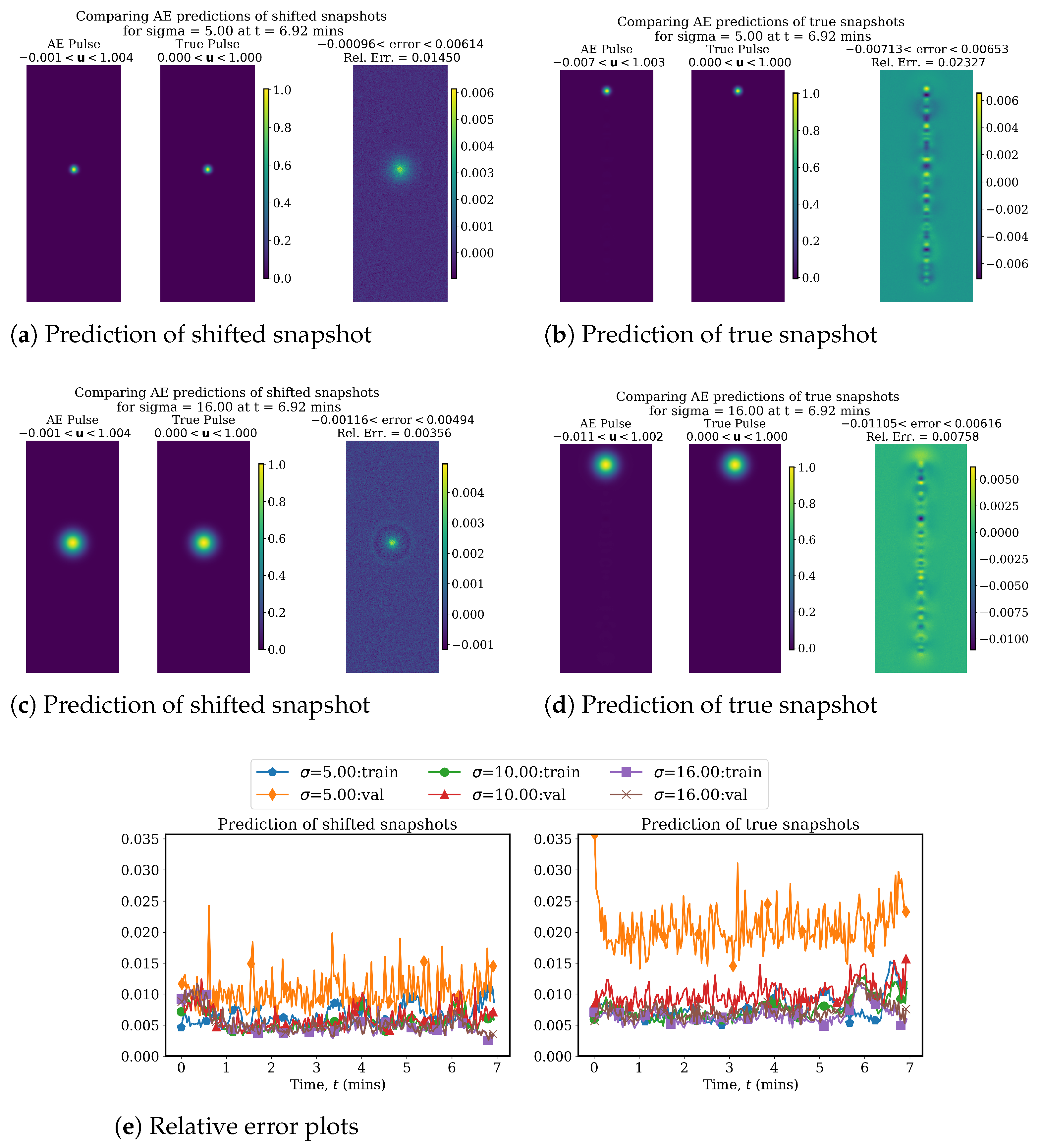
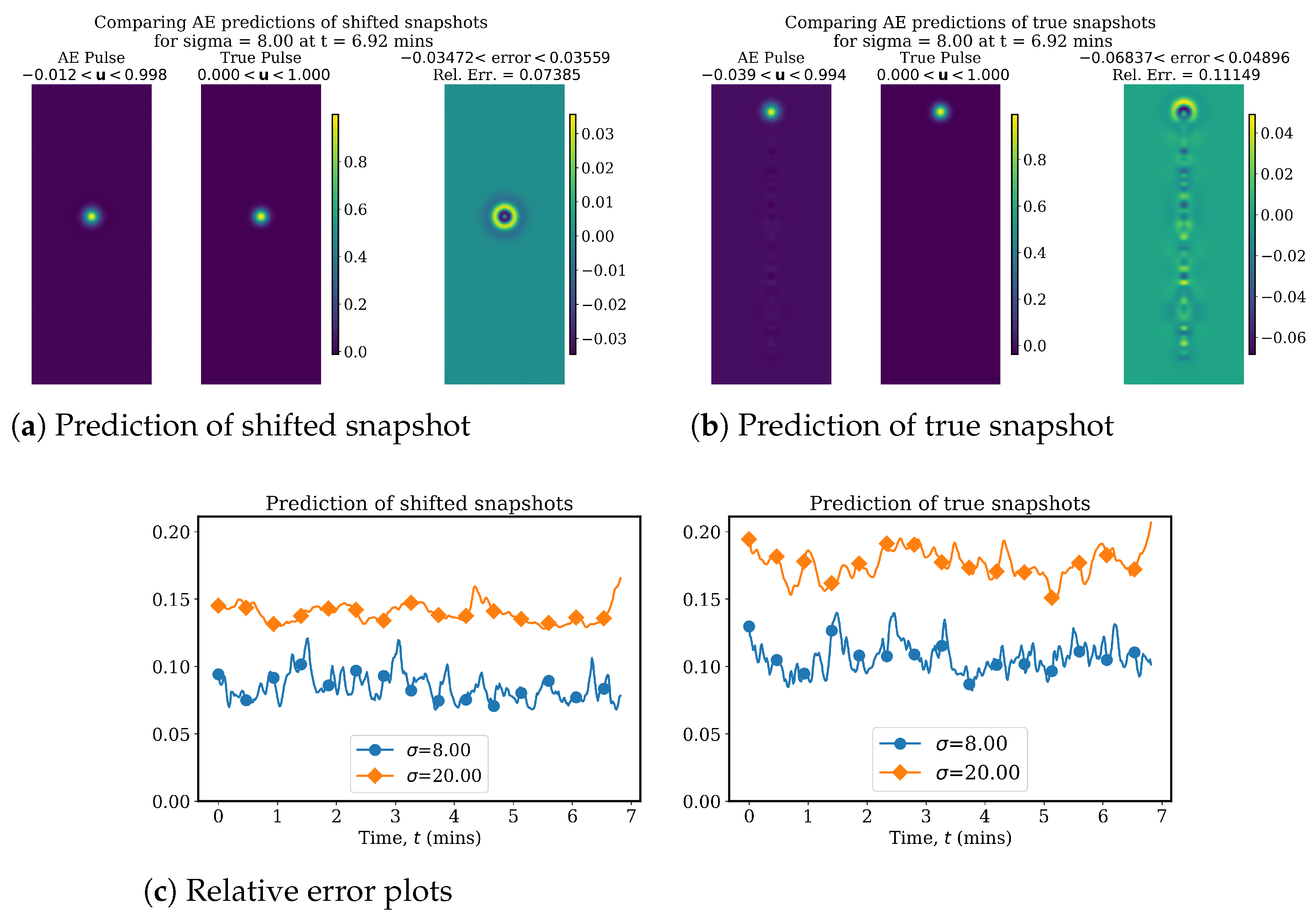
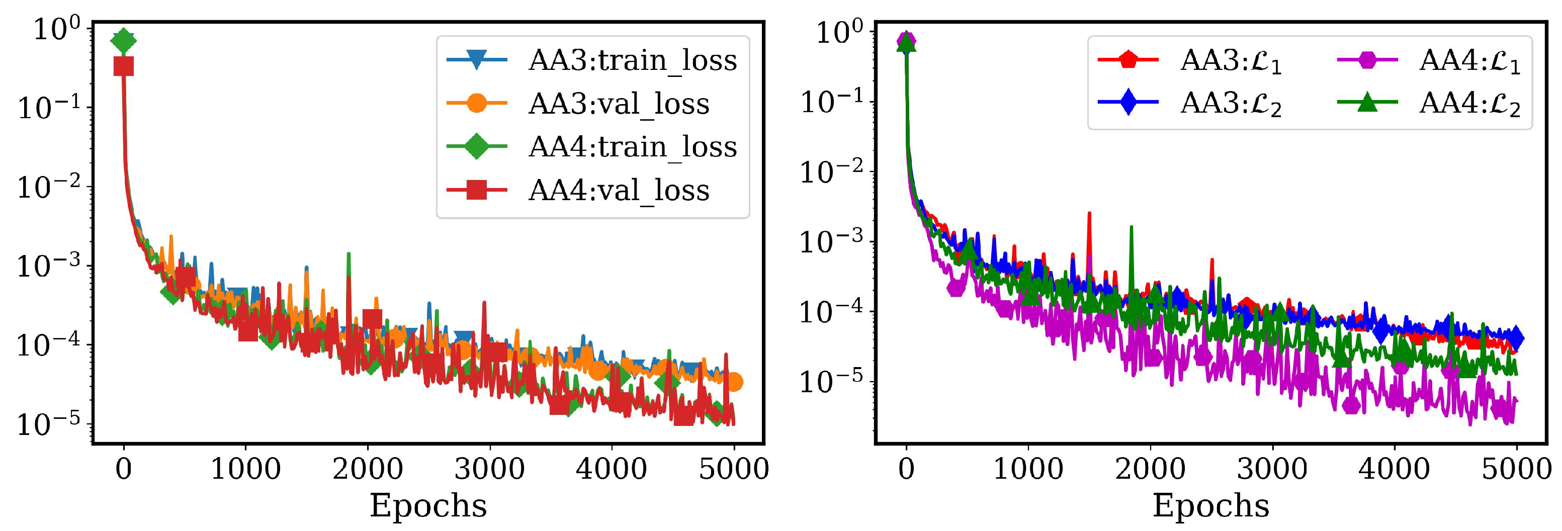
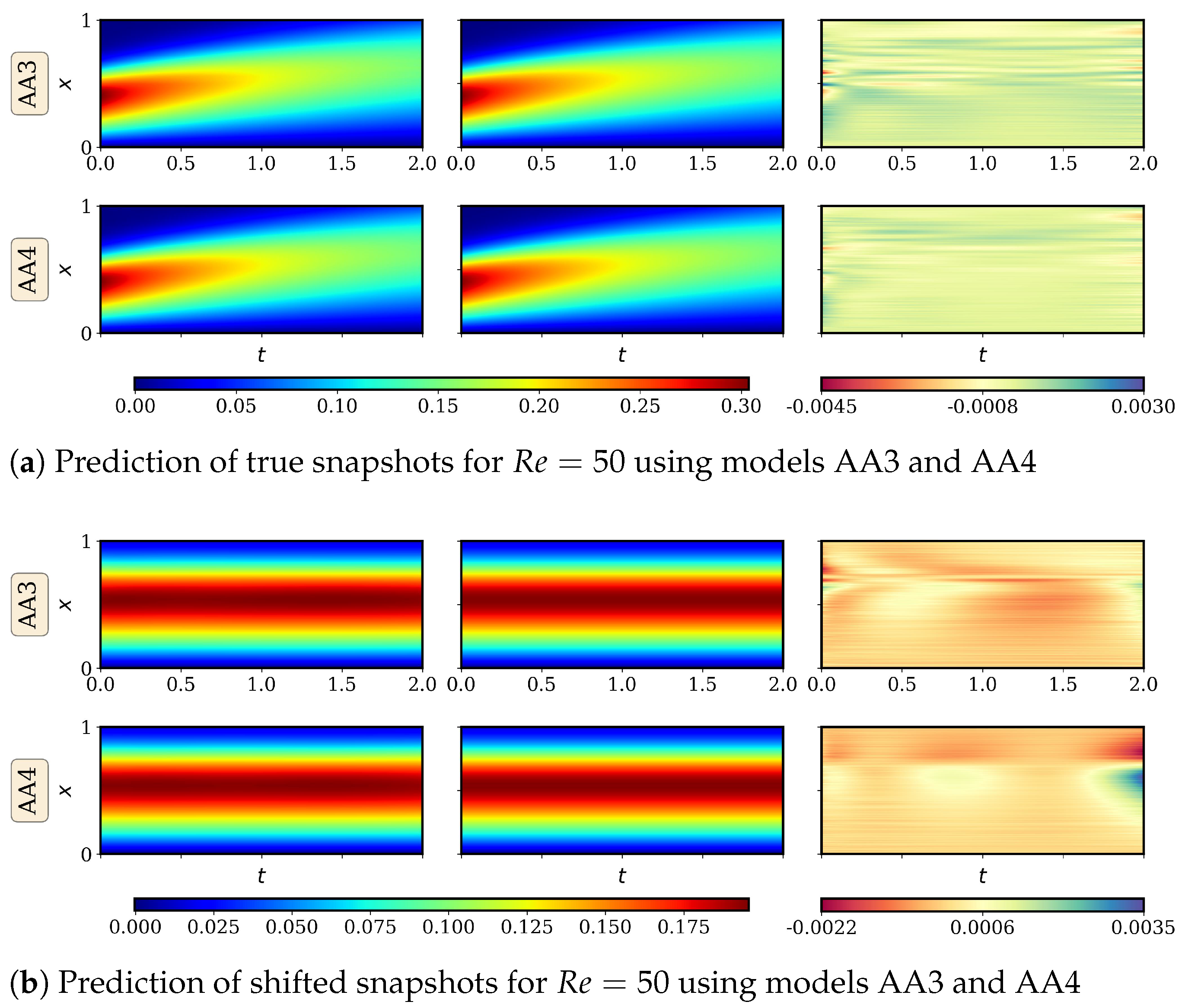
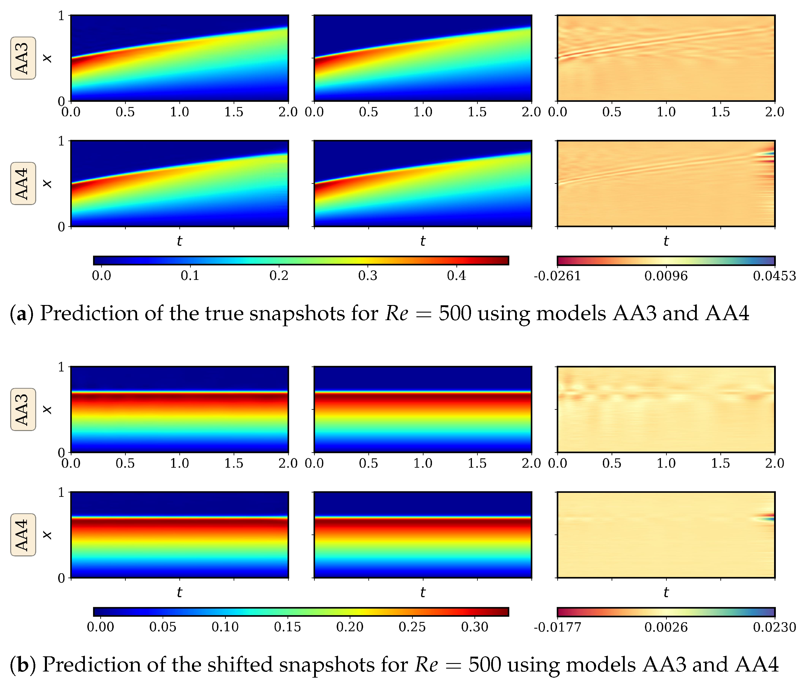
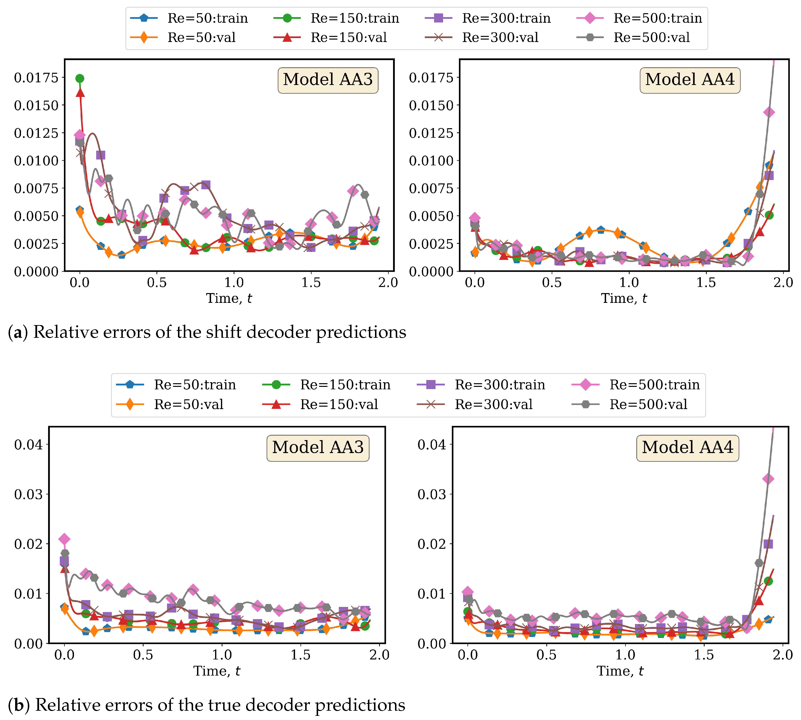
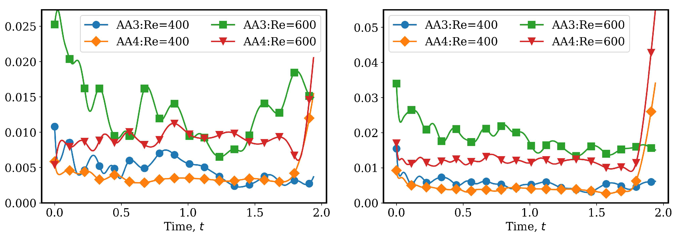
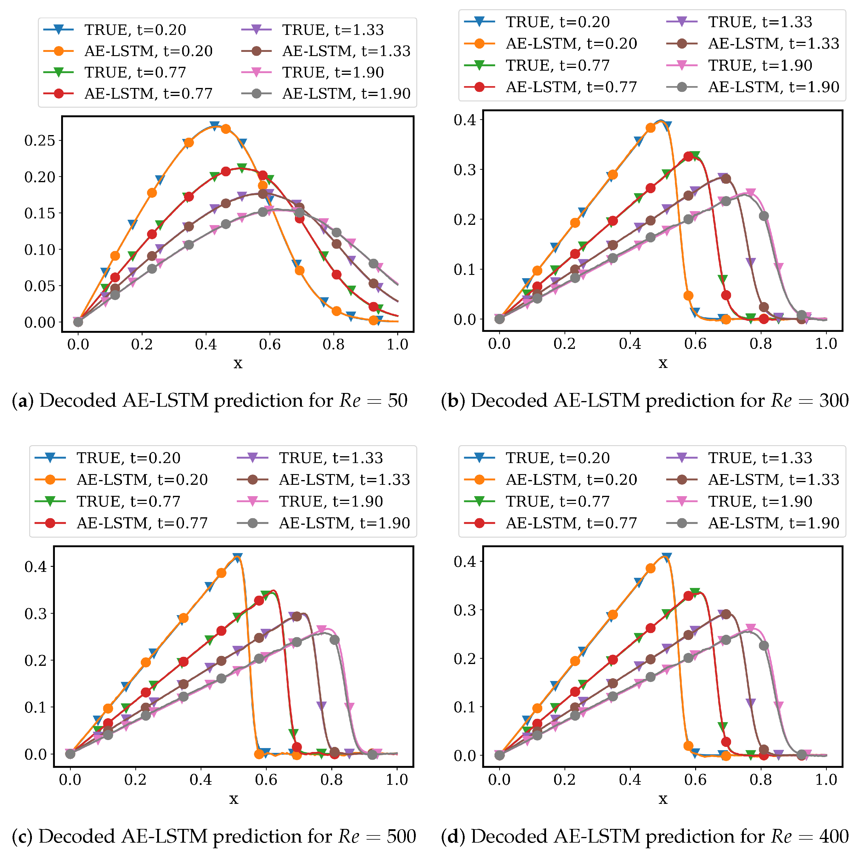
4.2.1. AA Autoencoder Models for Varying Advection Strength
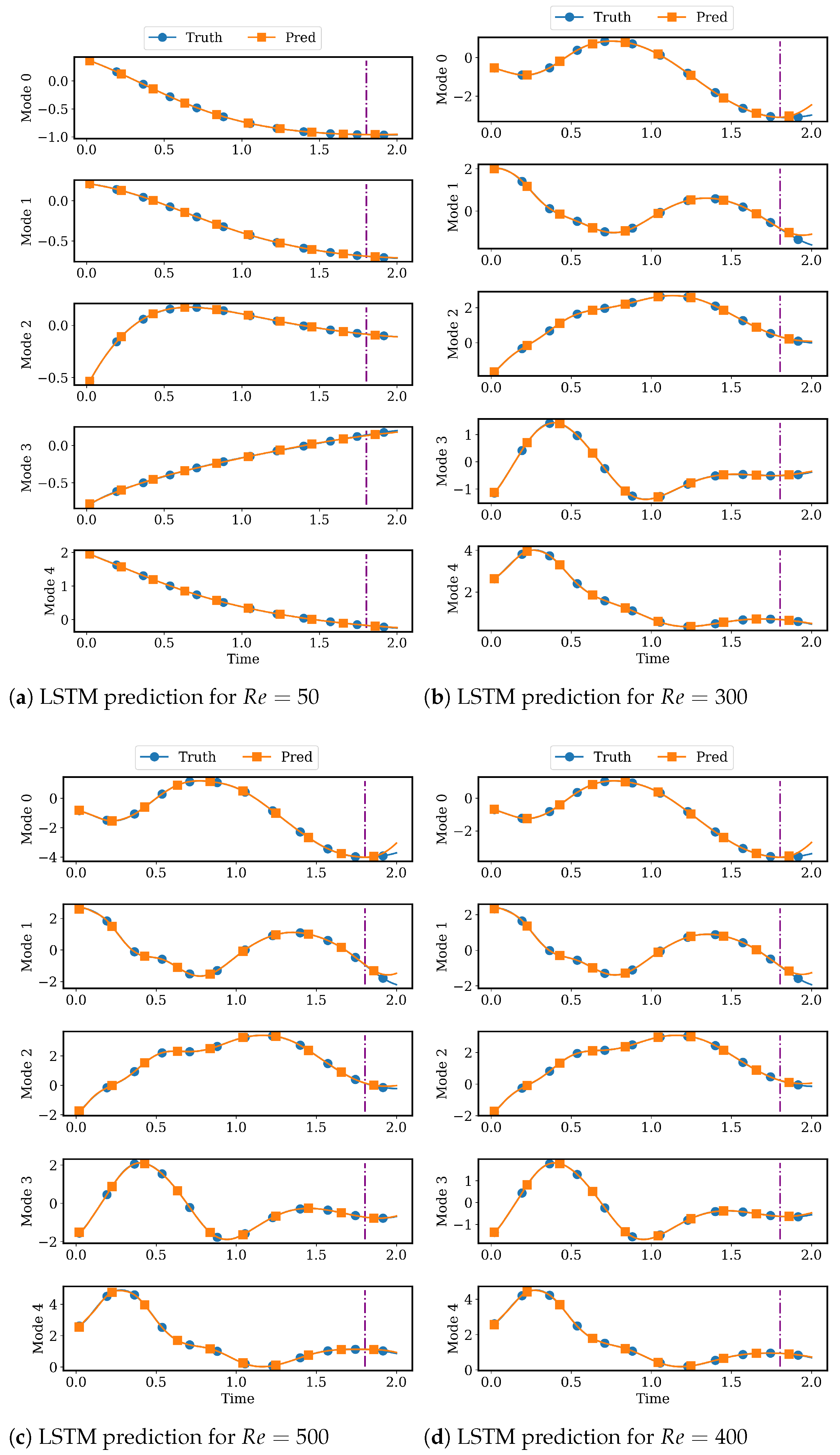
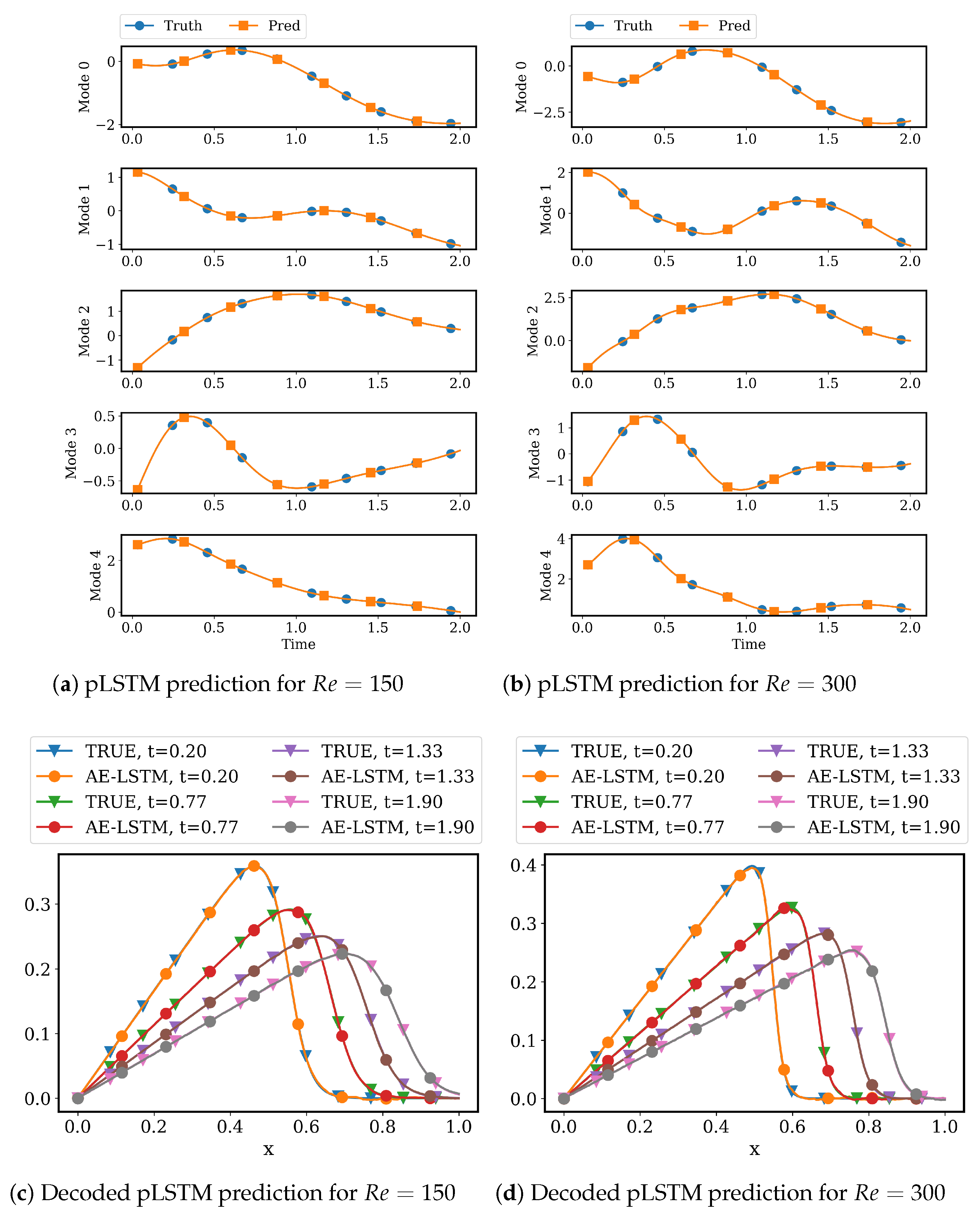
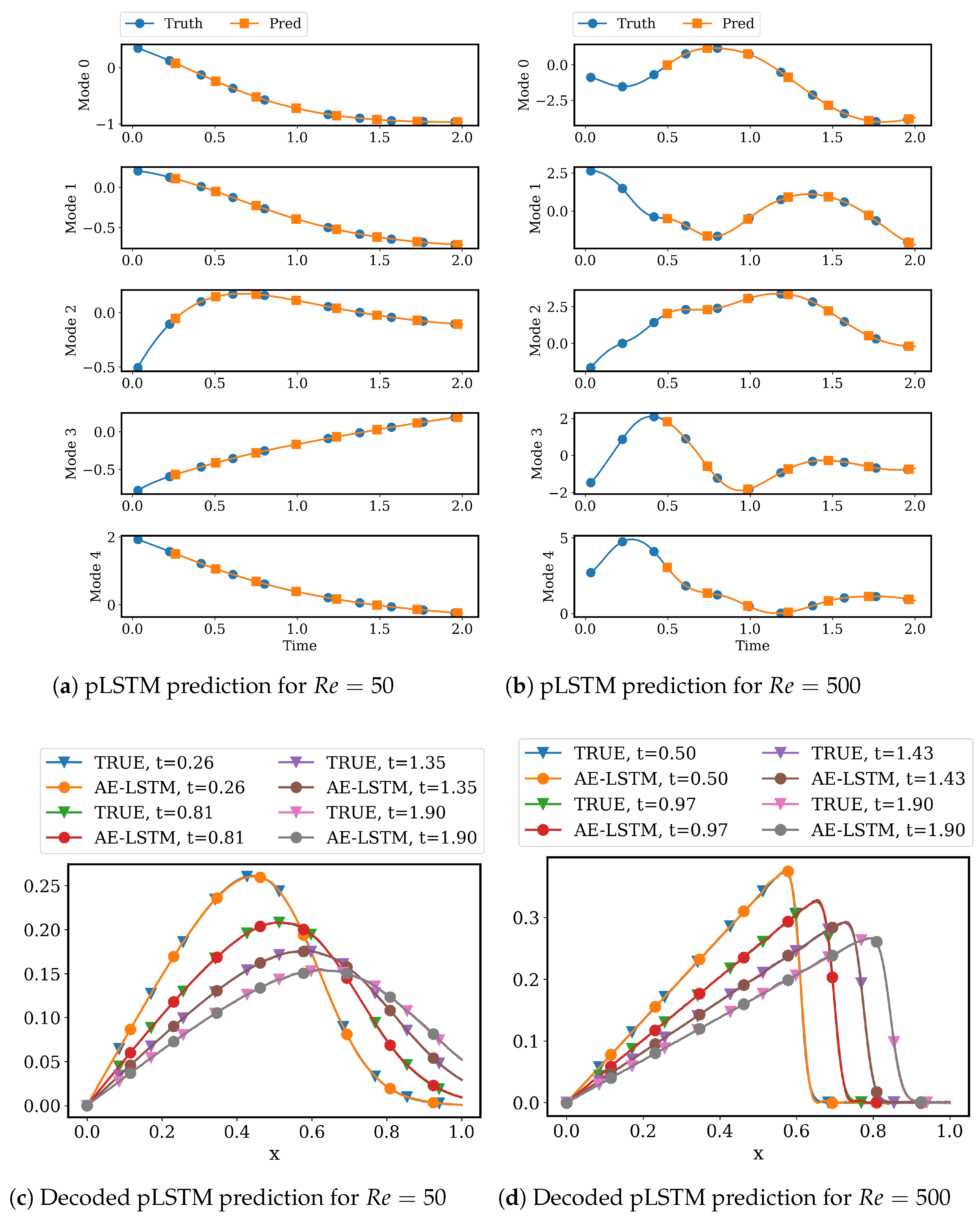
4.2.2. LSTM Models for System Dynamics
5. Conclusions and Future Work
Author Contributions
Funding
Data Availability Statement
Acknowledgments
Conflicts of Interest
References
- Kutz, J.N. Data-Driven Modeling & Scientific Computation: Methods for Complex Systems & Big Data; Oxford University Press, Inc.: Oxford, UK, 2013. [Google Scholar]
- Holmes, P.; Lumley, J.L.; Berkooz, G. Turbulence, Coherent Structures, Dynamical Systems and Symmetry; Cambridge Monographs on Mechanics, Cambridge University Press: Cambridge, UK, 1996. [Google Scholar] [CrossRef]
- Benner, P.; Gugercin, S.; Willcox, K. A Survey of Projection-Based Model Reduction Methods for Parametric Dynamical Systems. SIAM Rev. 2015, 57, 483–531. [Google Scholar] [CrossRef]
- Brunton, S.L.; Noack, B.R.; Koumoutsakos, P. Machine Learning for Fluid Mechanics. Annu. Rev. Fluid Mech. 2020, 52, 477–508. [Google Scholar] [CrossRef] [Green Version]
- Hesthaven, J.S.; Rozza, G.; Stamm, B. Certified Reduced Basis Methods for Parametrized Partial Differential Equations; Springer: Cham, Switzerland, 2016; pp. 1–131. [Google Scholar] [CrossRef] [Green Version]
- Rowley, C.W.; Dawson, S.T. Model Reduction for Flow Analysis and Control. Annu. Rev. Fluid Mech. 2017, 49, 387–417. [Google Scholar] [CrossRef] [Green Version]
- Taira, K.; Brunton, S.L.; Dawson, S.T.; Rowley, C.W.; Colonius, T.; McKeon, B.J.; Schmidt, O.T.; Gordeyev, S.; Theofilis, V.; Ukeiley, L.S. Modal analysis of fluid flows: An overview. AIAA J. 2017, 55, 4013–4041. [Google Scholar] [CrossRef] [Green Version]
- Berkooz, G.; Holmes, P.; Lumley, J.L. The proper orthogonal decomposition in the analysis of turbulent flows. Annu. Rev. Fluid Mech. 1993, 25, 539–575. [Google Scholar] [CrossRef]
- Lozovskiy, A.; Farthing, M.; Kees, C.; Gildin, E. POD-based model reduction for stabilized finite element approximations of shallow water flows. J. Comput. Appl. Math. 2016, 302, 50–70. [Google Scholar] [CrossRef]
- Lozovskiy, A.; Farthing, M.; Kees, C. Evaluation of Galerkin and Petrov–Galerkin model reduction for finite element approximations of the shallow water equations. Comput. Methods Appl. Mech. Eng. 2017, 318, 537–571. [Google Scholar] [CrossRef]
- Carlberg, K.; Barone, M.; Antil, H. Galerkin v. least-squares Petrov–Galerkin projection in nonlinear model reduction. J. Comput. Phys. 2017, 330, 693–734. [Google Scholar] [CrossRef] [Green Version]
- Dutta, S.; Rivera-Casillas, P.; Cecil, O.; Farthing, M. pyNIROM—A suite of python modules for non-intrusive reduced order modeling of time-dependent problems. Softw. Impacts 2021, 10, 100129. [Google Scholar] [CrossRef]
- Alla, A.; Kutz, J.N. Nonlinear model order reduction via dynamic mode decomposition. SIAM J. Sci. Comput. 2017, 39, B778–B796. [Google Scholar] [CrossRef]
- Wu, Z.; Brunton, S.L.; Revzen, S. Challenges in Dynamic Mode Decomposition. J. R. Soc. Interface 2021, 18, 20210686. [Google Scholar] [CrossRef] [PubMed]
- Xiao, D.; Fang, F.; Pain, C.C.; Navon, I.M. A parameterized non-intrusive reduced order model and error analysis for general time-dependent nonlinear partial differential equations and its applications. Comput. Methods Appl. Mech. Eng. 2017, 317, 868–889. [Google Scholar] [CrossRef] [Green Version]
- Dutta, S.; Farthing, M.W.; Perracchione, E.; Savant, G.; Putti, M. A greedy non-intrusive reduced order model for shallow water equations. J. Comput. Phys. 2021, 439, 110378. [Google Scholar] [CrossRef]
- Guo, M.; Hesthaven, J.S. Data-driven reduced order modeling for time-dependent problems. Comput. Methods Appl. Mech. Eng. 2019, 345, 75–99. [Google Scholar] [CrossRef]
- Xiao, D. Error estimation of the parametric non-intrusive reduced order model using machine learning. Comput. Methods Appl. Mech. Eng. 2019, 355, 513–534. [Google Scholar] [CrossRef]
- Hesthaven, J.S.; Ubbiali, S. Non-intrusive reduced order modeling of nonlinear problems using neural networks. J. Comput. Phys. 2018, 363, 55–78. [Google Scholar] [CrossRef] [Green Version]
- Wan, Z.Y.; Vlachas, P.; Koumoutsakos, P.; Sapsis, T. Data-assisted reduced-order modeling of extreme events in complex dynamical systems. PLoS ONE 2018, 13, e0197704. [Google Scholar] [CrossRef]
- Maulik, R.; Mohan, A.; Lusch, B.; Madireddy, S.; Balaprakash, P.; Livescu, D. Time-series learning of latent-space dynamics for reduced-order model closure. Phys. D Nonlinear Phenom. 2020, 405, 132368. [Google Scholar] [CrossRef] [Green Version]
- Chen, R.T.Q.; Rubanova, Y.; Bettencourt, J.; Duvenaud, D. Neural Ordinary Differential Equations. In Proceedings of the 32nd International Conference on Neural Information Processing Systems (NIPS’18), Montréal, QC, Canada, 2–8 December 2018; pp. 6572–6583. [Google Scholar] [CrossRef]
- Dutta, S.; Rivera-Casillas, P.; Farthing, M.W. Neural Ordinary Differential Equations for Data-Driven Reduced Order Modeling of Environmental Hydrodynamics. In Proceedings of the AAAI 2021 Spring Symposium on Combining Artificial Intelligence and Machine Learning with Physical Sciences, Virtual Meeting, 22–24 March 2021; CEUR-WS: Stanford, CA, USA, 2021. [Google Scholar]
- Wu, P.; Sun, J.; Chang, X.; Zhang, W.; Arcucci, R.; Guo, Y.; Pain, C.C. Data-driven reduced order model with temporal convolutional neural network. Comput. Methods Appl. Mech. Eng. 2020, 360, 112766. [Google Scholar] [CrossRef]
- Taddei, T.; Perotto, S.; Quarteroni, A. Reduced basis techniques for nonlinear conservation laws. ESAIM Math. Model. Numer. Anal. 2015, 49, 787–814. [Google Scholar] [CrossRef]
- Greif, C.; Urban, K. Decay of the Kolmogorov N-width for wave problems. Appl. Math. Letters 2019, 96, 216–222. [Google Scholar] [CrossRef] [Green Version]
- Carlberg, K.; Farhat, C.; Cortial, J.; Amsallem, D. The GNAT method for nonlinear model reduction: Effective implementation and application to computational fluid dynamics and turbulent flows. J. Comput. Phys. 2013, 242, 623–647. [Google Scholar] [CrossRef] [Green Version]
- Nair, N.J.; Balajewicz, M. Transported snapshot model order reduction approach for parametric, steady-state fluid flows containing parameter-dependent shocks. Int. J. Numer. Methods Eng. 2019, 117, 1234–1262. [Google Scholar] [CrossRef] [Green Version]
- Rim, D.; Moe, S.; LeVeque, R.J. Transport reversal for model reduction of hyperbolic partial differential equations. SIAM/ASA J. Uncertain. Quantif. 2018, 6, 118–150. [Google Scholar] [CrossRef] [Green Version]
- Reiss, J.; Schulze, P.; Sesterhenn, J.; Mehrmann, V. The shifted proper orthogonal decomposition: A mode decomposition for multiple transport phenomena. SIAM J. Sci. Comput. 2018, 40, A1322–A1344. [Google Scholar] [CrossRef] [Green Version]
- Rim, D.; Peherstorfer, B.; Mandli, K.T. Manifold approximations via transported subspaces: Model reduction for transport-dominated problems. arXiv 2019, arXiv:1912.13024. [Google Scholar]
- Cagniart, N.; Maday, Y.; Stamm, B. Model order reduction for problems with large convection effects. In Contributions to Partial Differential Equations and Applications; Springer International Publishing: Cham, Switzerland, 2019; pp. 131–150. [Google Scholar] [CrossRef] [Green Version]
- Taddei, T. A registration method for model order reduction: Data compression and geometry reduction. SIAM J. Sci. Comput. 2020, 42, A997–A1027. [Google Scholar] [CrossRef] [Green Version]
- Peherstorfer, B. Model reduction for transport-dominated problems via online adaptive bases and adaptive sampling. SIAM J. Sci. Comput. 2020, 42, A2803–A2836. [Google Scholar] [CrossRef]
- Kashima, K. Nonlinear model reduction by deep autoencoder of noise response data. In Proceedings of the 2016 IEEE 55th Conference on Decision and Control (CDC), Las Vegas, NV, USA, 12–14 December 2016; pp. 5750–5755. [Google Scholar] [CrossRef]
- Lee, K.; Carlberg, K.T. Model reduction of dynamical systems on nonlinear manifolds using deep convolutional autoencoders. J. Comput. Phys. 2020, 404, 108973. [Google Scholar] [CrossRef] [Green Version]
- Kim, Y.; Choi, Y.; Widemann, D.; Zohdi, T. A fast and accurate physics-informed neural network reduced order model with shallow masked autoencoder. J. Comput. Phys. 2022, 451, 110841. [Google Scholar] [CrossRef]
- Willcox, K. Unsteady flow sensing and estimation via the gappy proper orthogonal decomposition. Comput. Fluids 2006, 35, 208–226. [Google Scholar] [CrossRef] [Green Version]
- Chaturantabut, S.; Sorensen, D.C. Nonlinear model reduction via Discrete Empirical Interpolation. SIAM J. Sci. Comput. 2010, 32, 2737–2764. [Google Scholar] [CrossRef]
- Mendible, A.; Brunton, S.L.; Aravkin, A.Y.; Lowrie, W.; Kutz, J.N. Dimensionality reduction and reduced-order modeling for traveling wave physics. Theor. Comput. Fluid Dyn. 2020, 34, 385–400. [Google Scholar] [CrossRef]
- Haasdonk, B.; Ohlberger, M. Adaptive basis enrichment for the reduced basis method applied to finite volume schemes. In Proceedings of the Fifth International Symposium on Finite Volumes for Complex Applications, Aussois, France, 8–13 June 2008; pp. 471–479. [Google Scholar]
- Chen, P.; Quarteroni, A.; Rozza, G. A weighted empirical interpolation method: A priori convergence analysis and applications. ESAIM Math. Model. Numer. Anal. 2014, 48, 943–953. [Google Scholar] [CrossRef] [Green Version]
- Amsallem, D.; Farhat, C. An online method for interpolating linear parametric reduced-order models. SIAM J. Sci. Comput. 2011, 33, 2169–2198. [Google Scholar] [CrossRef]
- Maday, Y.; Stamm, B. Locally adaptive greedy approximations for anisotropic parameter reduced basis spaces. SIAM J. Sci. Comput. 2013, 35, A2417–A2441. [Google Scholar] [CrossRef] [Green Version]
- Peherstorfer, B.; Butnaru, D.; Willcox, K.; Bungartz, H.J. Localized discrete empirical interpolation method. SIAM J. Sci. Comput. 2014, 36, A168–A192. [Google Scholar] [CrossRef]
- Carlberg, K. Adaptive h-refinement for reduced-order models. Int. J. Numer. Methods Eng. 2015, 102, 1192–1210. [Google Scholar] [CrossRef] [Green Version]
- Peherstorfer, B.; Willcox, K. Online adaptive model reduction for nonlinear systems via low-rank updates. SIAM J. Sci. Comput. 2015, 37, A2123–A2150. [Google Scholar] [CrossRef]
- Tenenbaum, J. Mapping a manifold of perceptual observations. In Advances in Neural Information Processing Systems; Jordan, M., Kearns, M., Solla, S., Eds.; MIT Press: Cambridge, MA, USA, 1998; Volume 10. [Google Scholar]
- Roweis, S.T.; Saul, L.K. Nonlinear dimensionality reduction by locally linear embedding. Science 2000, 290, 2323–2326. [Google Scholar] [CrossRef] [Green Version]
- Belkin, M.; Niyogi, P. Laplacian eigenmaps for dimensionality reduction and data representation. Neural Comput. 2003, 15, 1373–1396. [Google Scholar] [CrossRef] [Green Version]
- van der Maaten, L.; Hinton, G. Visualizing data using t-SNE. J. Mach. Learn. Res. 2008, 9, 2579–2605. [Google Scholar]
- Kohonen, T. Self-organized formation of topologically correct feature maps. Biol. Cybern. 1982, 43, 59–69. [Google Scholar] [CrossRef]
- Mika, S.; Schölkopf, B.; Smola, A.; Müller, K.R.; Scholz, M.; Rätsch, G. Kernel PCA and de-noising in feature spaces. In Advances in Neural Information Processing Systems; Kearns, M., Solla, S., Cohn, D., Eds.; MIT Press: Cambridge, MA, USA, 1999; Volume 11. [Google Scholar]
- Walder, C.; Schölkopf, B. Diffeomorphic dimensionality reduction. In Advances in Neural Information Processing Systems 21; Koller, D., Schuurmans, D., Bengio, Y., Bottou, L., Eds.; Curran Associates Inc.: Red Hook, NY, USA, 2009; pp. 1713–1720. [Google Scholar]
- Hinton, G.E.; Salakhutdinov, R.R. Reducing the dimensionality of data with neural networks. Science 2006, 313, 504–507. [Google Scholar] [CrossRef] [PubMed] [Green Version]
- Masci, J.; Meier, U.; Cireşan, D.; Schmidhuber, J. Stacked Convolutional Auto-Encoders for Hierarchical Feature Extraction. In Artificial Neural Networks and Machine Learning—ICANN 2011; Honkela, T., Duch, W., Girolami, M., Kaski, S., Eds.; Springer: Berlin/Heidelberg, Germany, 2011; pp. 52–59. [Google Scholar]
- Radford, A.; Metz, L.; Chintala, S. Unsupervised representation learning with deep convolutional generative adversarial networks. In Proceedings of the 4th International Conference on Learning Representations (ICLR 2016), San Juan, Puerto Rico, 2–4 May 2016; pp. 1–16. [Google Scholar]
- Champion, K.; Lusch, B.; Nathan Kutz, J.; Brunton, S.L. Data-driven discovery of coordinates and governing equations. Proc. Natl. Acad. Sci. USA 2019, 116, 22445–22451. [Google Scholar] [CrossRef] [Green Version]
- Dutta, S.; Rivera-Casillas, P.; Cecil, O.M.; Farthing, M.W.; Perracchione, E.; Putti, M. Data-driven reduced order modeling of environmental hydrodynamics using deep autoencoders and neural ODEs. arXiv 2021, arXiv:2107.02784. [Google Scholar]
- Maulik, R.; Lusch, B.; Balaprakash, P. Reduced-order modeling of advection-dominated systems with recurrent neural networks and convolutional autoencoders. Phys. Fluids 2021, 33, 037106. [Google Scholar] [CrossRef]
- Wehmeyer, C.; Noé, F. Time-lagged autoencoders: Deep learning of slow collective variables for molecular kinetics. J. Chem. Phys. 2018, 148, 241703. [Google Scholar] [CrossRef] [Green Version]
- Nishizaki, H. Data augmentation and feature extraction using variational autoencoder for acoustic modeling. In Proceedings of the 2017 Asia-Pacific Signal and Information Processing Association Annual Summit and Conference (APSIPA ASC), Kuala Lumpur, Malaysia, 12–15 December 2017; pp. 1222–1227. [Google Scholar] [CrossRef]
- Bakarji, J.; Champion, K.; Kutz, J.N.; Brunton, S.L. Discovering Governing Equations from Partial Measurements with Deep Delay Autoencoders. arXiv 2022, arXiv:2201.05136. [Google Scholar]
- Erichson, N.B.; Muehlebach, M.; Mahoney, M.W. Physics-informed Autoencoders for Lyapunov-stable Fluid Flow Prediction. arXiv 2019, arXiv:1905.10866. [Google Scholar]
- Gonzalez, F.J.; Balajewicz, M. Deep convolutional recurrent autoencoders for learning low-dimensional feature dynamics of fluid systems. arXiv 2018, arXiv:1808.01346. [Google Scholar]
- Mojgani, R.; Balajewicz, M. Low-Rank Registration Based Manifolds for Convection-Dominated PDEs. In Proceedings of the Thirty-Fifth AAAI Conference on Artificial Intelligence (AAAI-21), Vancouver, BC, Canada, 2–9 February 2021; pp. 399–407. [Google Scholar]
- Plaut, E. From Principal Subspaces to Principal Components with Linear Autoencoders. arXiv 2018, arXiv:1804.10253. [Google Scholar]
- Greff, K.; Srivastava, R.K.; Koutník, J.; Steunebrink, B.R.; Schmidhuber, J. LSTM: A search space odyssey. IEEE Trans. Neural Netw. Learn. Syst. 2016, 28, 2222–2232. [Google Scholar] [CrossRef] [Green Version]
- Eivazi, H.; Veisi, H.; Naderi, M.H.; Esfahanian, V. Deep neural networks for nonlinear model order reduction of unsteady flows. Phys. Fluids 2020, 32, 105104. [Google Scholar] [CrossRef]
- Maulik, R.; Lusch, B.; Balaprakash, P. Non-autoregressive time-series methods for stable parametric reduced-order models. Phys. Fluids 2020, 32, 087115. [Google Scholar] [CrossRef]
- del Águila Ferrandis, J.; Triantafyllou, M.S.; Chryssostomidis, C.; Karniadakis, G.E. Learning functionals via LSTM neural networks for predicting vessel dynamics in extreme sea states. Proc. R. Soc. A 2021, 477, 20190897. [Google Scholar] [CrossRef]
- Chattopadhyay, A.; Mustafa, M.; Hassanzadeh, P.; Kashinath, K. Deep Spatial Transformers for Autoregressive Data-Driven Forecasting of Geophysical Turbulence. In Proceedings of the 10th International Conference on Climate Informatics, Oxford, UK, 22–25 September 2020; Association for Computing Machinery: New York, NY, USA, 2020; pp. 106–112. [Google Scholar] [CrossRef]
- Pathak, J.; Hunt, B.; Girvan, M.; Lu, Z.; Ott, E. Model-Free Prediction of Large Spatiotemporally Chaotic Systems from Data: A Reservoir Computing Approach. Phys. Rev. Lett. 2018, 120, 24102. [Google Scholar] [CrossRef] [Green Version]
- Usman, A.; Rafiq, M.; Saeed, M.; Nauman, A.; Almqvist, A.; Liwicki, M. Machine learning-accelerated computational fluid dynamics. Proc. Natl. Acad. Sci. USA 2021, 118, e2101784118. [Google Scholar] [CrossRef]
- Stabile, G.; Zancanaro, M.; Rozza, G. Efficient geometrical parametrization for finite-volume-based reduced order methods. Int. J. Numer. Methods Eng. 2020, 121, 2655–2682. [Google Scholar] [CrossRef]


| Hyperparameters | AA1 | AA2 |
|---|---|---|
| Input/Output | Augmented Input, non-augmented output | Augmented input and output |
| Hidden Units (50–1500) | ||
| Batch Size (8–128) | 32 | 24 |
| Latent Dimension (5–50) | 15 | 15 |
| Activation (ReLU, selu, linear, tanh, swish) | selu | swish |
| Hyperparameters | AA3 | AA4 |
|---|---|---|
| Input/Output | Augmented input and output | Augmented input and output |
| Hidden Units (50–150) | 50 | |
| Batch Size (8–128) | 24 | 24 |
| Latent Dimension (3–10) | 5 | 5 |
| Activation (selu, tanh, swish) | swish | swish |
| Initial Learning Rate (–) |
Publisher’s Note: MDPI stays neutral with regard to jurisdictional claims in published maps and institutional affiliations. |
© 2022 by the authors. Licensee MDPI, Basel, Switzerland. This article is an open access article distributed under the terms and conditions of the Creative Commons Attribution (CC BY) license (https://creativecommons.org/licenses/by/4.0/).
Share and Cite
Dutta, S.; Rivera-Casillas, P.; Styles, B.; Farthing, M.W. Reduced Order Modeling Using Advection-Aware Autoencoders. Math. Comput. Appl. 2022, 27, 34. https://doi.org/10.3390/mca27030034
Dutta S, Rivera-Casillas P, Styles B, Farthing MW. Reduced Order Modeling Using Advection-Aware Autoencoders. Mathematical and Computational Applications. 2022; 27(3):34. https://doi.org/10.3390/mca27030034
Chicago/Turabian StyleDutta, Sourav, Peter Rivera-Casillas, Brent Styles, and Matthew W. Farthing. 2022. "Reduced Order Modeling Using Advection-Aware Autoencoders" Mathematical and Computational Applications 27, no. 3: 34. https://doi.org/10.3390/mca27030034