Equity Warrants Pricing Formula for Uncertain Financial Market

Abstract

In this paper, inside the system of uncertainty theory, the valuation of equity warrants is explored. Different from the strategies of probability theory, the valuation problem of equity warrants is unraveled by utilizing the strategy of uncertain calculus. Based on the suspicion that the firm price follows an uncertain differential equation, a valuation formula of equity warrants is proposed for an uncertain stock model.

1. Introduction

Warrants give the holder the right but not the obligation to purchase or sell the underlying assets by a specific date for a certain cost. Be that as it may, this right is not free. The warrant is one sort of exceptional option and it can be ordered in many types. Warrants can be partitioned into American warrants and European warrants as indicated by the distinction of the lapse date. Furthermore, they may be partitioned into call warrants and put warrants as indicated by the distinction of activity method. They may also be partitioned into equity warrants and covered warrants, agreeing with the distinction of the issuer. Covered warrants are as a rule given by sellers, which do not raise the organization’s capital stock after their lapse dates. Valuing for this sort of warrant is like evaluating for normal options and, subsequently, numerous specialists use the Black–Scholes model [1] to value this sort of warrant. Yet, the value warrants are generally given by the recorded organization and the underlying capital is the given stock of its organization. The value warrants have a weakening impact and, consequently, valuing for this sort of warrant is in contrast to estimating for the standard European options in light of the fact that the organizations’ equity warrants need to give new stock to meet the solicitation of the warrants’ holder at the maturity date. All in all, the estimation cannot totally apply the works of art Black–Scholes model.

Uncertainty strategy was established by Liu [2] in 2007, and it has turned into a part of obvious mathematics for demonstrating belief degrees. As a part of obvious mathematics to manage belief degrees, the uncertainty hypothesis will assume a significant part in financial hypothesis and practice. Liu [3] started the pioneering work of uncertain finance in 2009. Thereafter, numerous analysts applied themselves to an investigation of financial issues by utilizing uncertainty strategy. For instance, Chen [4] explored the American alternative estimating issue and determined the evaluating formulae for Liu’s uncertain stock model, and Chen and Gao [5] presented an uncertain term structure model of interest rate. Plus, in view of uncertainty strategy, Chen, Liu, and Ralescu [6] proposed an uncertain stock model with intermittent profits.

Previous studies of pricing equity warrants were mainly carried out with the method of stochastic finance based on the probability theory, and the firm price was usually assumed to follow some stochastic differential equation [7,8,9]. However, many empirical investigations showed that the firm value does not behave randomly, and it is often influenced by the belief degrees of investors since investors usually make their decisions based on the degrees of belief rather than the probabilities. For example, one of the key elements in the Nobel Prize-winning theory of Kahneman and Tversky [10,11] is the finding of probability distortion which showed that decision makers usually make their decisions based on a nonlinear transformation of the probability scale rather than the probability itself, and people often overweight small probabilities and underweight large probabilities. Actually, we know that investors’ belief degrees play an important role in decision making for financial practice [12,13,14]. Although a few models have been utilized in an equity warrant pricing, applying an uncertain stock strategy has not been considered. In this paper, inside the system of uncertain hypotheses, we examine the pricing issue of equity warrants. Based on the suspicion that the stock price satisfies an uncertain differential equation, we derive an uncertain model for estimating equity warrants.

The remainder of the paper is organized as follows: Some fundamental ideas of uncertain processes are reviewed in Section 2. In Section 3, a short presentation of an uncertain stock model is given. An uncertain value warrants model is proposed in Section 4. Finally, a concise rundown is given in Section 5.

2. Preliminary

A uncertain process is basically a sequence of uncertain variables indexed by time or space. In this segment, we review some essential realities about uncertain processes.

Definition 1

([15]). Let T be an index set and let $(\Gamma ,\mathcal{M},\mathcal{L})$ be an uncertainty space. An uncertain process is a measurable function from $T\times (\Gamma ,\mathcal{M},\mathcal{L})$ to the set of real numbers, i.e., for each $t\in T$ and any Borel set B of real numbers, the set

$$\begin{array}{c}\hfill \{X_t\in B\}=\{\gamma \in \Gamma |X_t\left(\gamma \right)\in B\}\end{array}$$

is an event.

Definition 2

([15]). The uncertainty distribution Φ of an uncertain variable ξ is defined by

$$\begin{array}{c}\hfill \Phi \left(x\right)=\mathcal{M}\{\xi \le x\}\end{array}$$

for any real number x.

Definition 3

([15]). An uncertain variable ξ is called normal if it has a normal uncertainty distribution

$$\begin{array}{c}\hfill \Phi \left(x\right)={\left(1+exp\left(\frac{\pi (e-x)}{\sqrt{3}\sigma }\right)\right)}^{-1}\end{array}$$

denoted by $\mathcal{N}(e,\sigma )$ where e and σ are real numbers with $\sigma >0$.

Definition 4

([2]). Let ξ be an uncertain variable. Then, the expected value of ξ is defined by

$$\begin{array}{c}\hfill E\left[\xi \right]={\int }_0^{+\infty }\mathcal{M}\{\xi \ge r\}dr-{\int }_{-\infty }^0\mathcal{M}\{\xi \le r\}dr,\end{array}$$

provided that at least one of the two integrals is finite.

Theorem 1

([2]). Let ξ be an uncertain variable with uncertainty distribution Φ. If the expected value exists, then

$$\begin{array}{c}\hfill E\left[\xi \right]={\int }_0^{+\infty }(1-\Phi \left(x\right))dx-{\int }_{-\infty }^0\Phi \left(x\right)dx.\end{array}$$

Theorem 2

([16]). Let ξ be an uncertain variable with regular uncertainty distribution Φ. Then,

$$\begin{array}{c}\hfill E\left[\xi \right]={\int }_0^1{\Phi }^{-1}\left(\alpha \right)d\alpha .\end{array}$$

Definition 5

([17]). Let $C_t$ be a canonical Liu process and let $Z_t$ be an uncertain process. If there exist uncertain processes ${\mu }_t$ and ${\sigma }_t$ such that

$$\begin{array}{c}\hfill Z_t=Z_0+{\int }_0^t{\mu }_{s}ds+{\int }_0^t{\sigma }_{s}d{C}_s,\end{array}$$

for any $t\ge 0$, then $Z_t$ is called a Liu process with drift ${\mu }_t$ and diffusion ${\sigma }_t$. Furthermore, $Z_t$ has an uncertain differential

$$\begin{array}{c}\hfill d{Z}_t={\mu }_{t}dt+{\sigma }_{t}d{C}_t.\end{array}$$

Definition 6

([15]). Suppose $C_t$ is a canonical Liu process, and f and g are two functions. Then,

$$\begin{array}{c}\hfill d{X}_t=f(t,X_t)dt+g(t,X_t)d{C}_t\end{array}$$

is called an uncertain differential equation.

Definition 7

([18]). Let α be a number with $0<\alpha <1$. An uncertain differential equation

$$\begin{array}{c}\hfill d{X}_t=f(t,X_t)dt+g(t,X_t)d{C}_t\end{array}$$

is said to have an α-path $X_t^{\alpha }$ if it solves the corresponding ordinary differential equation

$$\begin{array}{c}\hfill d{X}_t^{\alpha }=f(t,X_t^{\alpha })dt+\left|g(t,X_t^{\alpha })\right|{\Phi }^{-1}\left(\alpha \right)dt,\end{array}$$

where ${\Phi }^{-1}\left(\alpha \right)$ is the inverse standard normal uncertainty distribution, i.e.,

$$\begin{array}{c}\hfill {\Phi }^{-1}\left(\alpha \right)=\frac{\sqrt{3}}{\pi }ln\frac{\alpha }{1-\alpha }.\end{array}$$

Theorem 3

([18]). Let $X_t$ and $X_t^{\alpha }$ be the solution and α-path of the uncertain differential equation

$$\begin{array}{c}\hfill d{X}_t=f(t,X_t)dt+g(t,X_t)d{C}_t,\end{array}$$

respectively. Then,

$$\begin{array}{ccc}\hfill \mathcal{M}\{X_t\le X_t^{\alpha },\forall t\}& =& \alpha \hfill \\ \hfill \mathcal{M}\{X_t>X_t^{\alpha },\forall t\}& =& 1-\alpha .\hfill \end{array}$$

Theorem 4

([18]). Let $X_t$ and $X_t^{\alpha }$ be the solution and α-path of the uncertain differential equation

$$\begin{array}{c}\hfill d{X}_t=f(t,X_t)dt+g(t,X_t)d{C}_t,\end{array}$$

respectively. Then, the solution $X_t$ has an inverse uncertainty distribution

$$\begin{array}{c}\hfill {\Psi }_t^{-1}\left(\alpha \right)=X_t^{\alpha }.\end{array}$$

Theorem 5

([18]). Let $X_t$ and $X_t^{\alpha }$ be the solution and α-path of the uncertain differential equation

$$\begin{array}{c}\hfill d{X}_t=f(t,X_t)dt+g(t,X_t)d{C}_t,\end{array}$$

respectively. Then, for any monotone (increasing or decreasing) function I, we have

$$\begin{array}{c}\hfill E\left[I\left(X_t\right)\right]={\int }_0^{1}I\left(X_t^{\alpha }\right)d\alpha .\end{array}$$

3. Uncertain Stock Model

Since the pioneer papers of Black, Scholes, and Merton on option evaluation were distributed in the mid-1970s, as a significant instrument, the Black–Scholes model was broadly utilized for estimating the financial derivatives by numerous specialists in which the stock value measure was portrayed by a stochastic differential equation as follows:

$$\left\{\begin{array}{c}d{X}_t=r{X}_{t}dt\hfill \\ d{V}_t=\mu V_{t}dt+\sigma V_{t}d{B}_t,\hfill \end{array}\right.$$

(1)

where $X_t$ is the bond price, $V_t$ is the stock price, r is the riskless interest rate, $\mu$ is the log-drift, $\sigma$ is the log-diffusion, and $B_t$ is a Wiener process.

Nonetheless, this assumption was tested among others by Liu [17] who proposed a contradiction showing that utilizing stochastic differential equations to depict stock value processes is not sensible. As an alternate tenet, Liu [3] generalized an uncertain differential equation to portray the fundamental stock value process and derived an uncertain stock model in which the bond value $X_t$ and the stock cost $V_t$ are described by

$$\left\{\begin{array}{c}d{X}_t=r{X}_{t}dt\hfill \\ d{V}_t=\mu V_{t}dt+\sigma V_{t}d{C}_t,\hfill \end{array}\right.$$

(2)

where $C_t$ is a Liu process.

It follows from Equation (2) that the stock price is

$$\begin{array}{c}\hfill V_t=V_0{e}^{\mu t+\sigma C_t},0\le t\le T,\end{array}$$

(3)

whose inverse uncertainty distribution is

$$\begin{array}{c}\hfill {\Phi }^{-1}\left(\alpha \right)=V_{0}exp\left\{\mu t+\frac{\sigma t\sqrt{3}}{\pi }ln\frac{\alpha }{1-\alpha }\right\}.\end{array}$$

4. The Pricing Model

Given an uncertainty space $(\Gamma ,\mathcal{M},\mathcal{L})$, we will suppose ideal conditions in the market for the firm’s value and for the equity warrants:

(i)

There are no transaction costs or taxes and all securities are perfectly divisible.

(ii)

Dividends are not paid during the lifetime of the outstanding warrants, and the sequential exercise of the warrants is not optimal for warrant holders.

(iii)

The warrant-issuing firm is an equity firm with no outstanding debt.

(iv)

The total equity value of the firm, during the lifetime of the outstanding warrants, $V_t$, satisfies Equation (2).

In the case of equity warrants, the firm has N shares of common stock and M shares of equity warrants outstanding. Each warrant entitles the owner to receive k shares of stock at time T upon payment of J, the payoff of equity warrants is given by $\frac{1}{N+Mk}{[k{V}_T-NJ]}^{+}$, where $V_T$ is the value of the firm’s assets at time T. Considering the time value of money resulting from the bond, the present value of this payoff is

$$\begin{array}{c}\hfill \frac{e^{-r(T-t)}}{N+Mk}{[k{V}_T-NJ]}^{+}.\end{array}$$

Let $f_w$ represent the price of the equity warrant. Then, the time-zero net return of the warrant holder is

$$\begin{array}{c}\hfill -f_w+\frac{e^{-r(T-t)}}{N+Mk}{[k{V}_T-NJ]}^{+}.\end{array}$$

On the other hand, the time-zero net return of the issuer is

$$\begin{array}{c}\hfill f_w-\frac{e^{-r(T-t)}}{N+Mk}{[k{V}_T-NJ]}^{+}.\end{array}$$

The fair price of this contract should make the holder of the equity warrant and the bank have an identical expected return, i.e.,

$$\begin{array}{ccc}& & f_w-E\left[\frac{e^{-r(T-t)}}{N+Mk}{[k{V}_T-NJ]}^{+}\right]\hfill \\ & & =-f_w+E\left[\frac{e^{-r(T-t)}}{N+Mk}{[k{V}_T-NJ]}^{+}\right].\hfill \end{array}$$

Thus, the price of an equity warrant can be defined as follows.

Definition 8.

Assume that there is a firm financed by N shares of stock and M shares of equity warrants. Each warrant gives the holder the right to buy k shares of stock at time $t=T$ in exchange for payment of an amount J. Let $V_t$ be the asset value of the firm at time t. Then, the equity warrant price is

$$\begin{array}{c}\hfill f_w=\frac{e^{-r(T-t)}}{N+Mk}E\left[{(k{V}_T-NJ)}^{+}\right].\end{array}$$

Theorem 6.

Based on all information from Definition (8), the price of an equity warrant at time t is given by

$$\begin{array}{ccc}\hfill f_w& =& \frac{e^{-r(T-t)}}{N+Mk}{\int }_0^1[k{V}_{t}exp\{\mu (T-t)\hfill \\ & +& \frac{\sigma \sqrt{3}(T-t)}{\pi }ln\frac{\alpha }{1-\alpha }\}-NJ{]}^{+}d\alpha ,\hfill \end{array}$$

where the optimal solutions ${\sigma }^{*}$ and $V_t^{*}$ satisfy the following system of nonlinear equations:

$$\left\{\begin{array}{c}N{S}_t=V_t-M{f}_w\hfill \\ {\sigma }_s=\frac{\sigma V_t}{S_t}\left(\frac{1}{N}-\frac{M}{N}\frac{\partial f_w}{\partial V_t}\right).\hfill \end{array}\right.$$

(4)

Proof. 

Solving the ordinary differential equation

$$\begin{array}{c}\hfill d{V}_t^{\alpha }=\mu V_t^{\alpha }dt+\sigma V_t^{\alpha }{\Phi }^{-1}\left(\alpha \right)dt,\end{array}$$

where $0<\alpha <1$ and ${\Phi }^{-1}\left(\alpha \right)$ is the inverse standard normal uncertainty distribution, we have

$$\begin{array}{c}\hfill V_t^{\alpha }=V_{0}exp\left\{\mu t+\sigma {\Phi }^{-1}\left(\alpha \right)t\right\}.\end{array}$$

That means that the uncertain differential equation $d{V}_t=\mu V_{t}dt+\sigma V_{t}d{C}_t$ has an $\alpha$-path

$$\begin{array}{ccc}\hfill V_t^{\alpha }& =& V_{0}exp\left\{\mu t+\sigma {\Phi }^{-1}\left(\alpha \right)t\right\}\hfill \\ & =& V_{0}exp\left\{\mu t+\frac{\sigma \sqrt{3}}{\pi }ln\frac{\alpha }{1-\alpha }\right\}.\hfill \end{array}$$

Since $I\left(x\right)=\frac{e^{-r(T-t)}}{N+Mk}{[k{V}_T-NJ]}^{+}$ is an increasing function, it follows from Theorem 5 and Definition (8) that the equity warrant price is

$$\begin{array}{ccc}\hfill f_w& =& E\left[I\left(V_T\right)\right]={\int }_0^{1}I\left(V_T^{\alpha }\right)d\alpha \hfill \\ & =& \frac{e^{-r(T-t)}}{N+Mk}{\int }_0^1{\left[k{V}_T^{\alpha }-NJ\right]}^{+}d\alpha \hfill \\ & =& \frac{e^{-r(T-t)}}{N+Mk}{\int }_0^1[k{V}_{t}exp\{\mu (T-t)\hfill \\ & +& \frac{\sigma \sqrt{3}(T-t)}{\pi }ln\frac{\alpha }{1-\alpha }\}-NJ{]}^{+}d\alpha .\hfill \end{array}$$

It is shown that the warrant pricing formula mentioned above depends on $V_t$ and $\sigma$, which are unobservable. To obtain a pricing formula using observable values, we will make use of the following result.

Let $\beta$ be the stock’s elasticity, which gives the percentage change in the stock’s value for a percentage change in the firm’s value. Then, from a standard result in option pricing theory, we have

$$\begin{array}{c}\hfill \beta =\frac{{\sigma }_s}{\sigma }=\frac{V_t\partial S_t}{S_t\partial V_t}.\end{array}$$

(5)

From assumption (iii), we obtain $V_t=N{S}_t+M{f}_w$. Consequently, we have

$$\begin{array}{c}\hfill \frac{\partial S_t}{\partial V_t}=\frac{1}{N}-\frac{M}{N}\frac{\partial f_w}{\partial V_t}.\end{array}$$

(6)

Now, from (5) and (6), it follows that

$$\begin{array}{c}\hfill {\sigma }_s=\frac{\sigma V_t}{S_t}\left[\frac{1}{N}-\frac{M}{N}\frac{\partial f_w}{\partial V_t}\right].\end{array}$$

(7)

 □

Theorem 7.

If $0<\alpha <\frac{1}{2}$. Then, the nonlinear system (4) has a solution $({\sigma }^{*},V_t^{*})\in (0,+\infty )\times (0,+\infty )$.

Proof. 

First, it is clear that for any $\sigma \in (0,+\infty )$, there exists a unique $V_t\in (0,+\infty )$ which satisfies

$$\begin{array}{c}\hfill N{S}_t=V_t-M{f}_w.\end{array}$$

Define a map $g:\sigma \to V_t$, which is given by an implicit function

$$\begin{array}{c}\hfill G(\sigma ,V_t)=V_t-M{f}_w-N{S}_t.\end{array}$$

The function $g:\sigma \mapsto V_t$ is increasing when $0<\alpha <\frac{1}{2}$ since the following inequality holds:

$$\begin{array}{c}\hfill \frac{d{V}_t}{d\sigma }=-\frac{\partial G/\partial \sigma }{\partial G/\partial V_t}=\frac{M\frac{\partial f_w}{\partial \sigma }}{1-M\frac{\partial f_w}{\partial V_t}}>0.\end{array}$$

The inequality holds true because the function $f_w$ is an increasing function of $\sigma$.

Second, it is obvious that for any $\sigma \in (0,+\infty )$, there exists a unique $V_t\left(\sigma \right)\in (0,+\infty )$, which satisfies

$$\begin{array}{c}\hfill {\sigma }_s=\frac{\sigma V_t}{S_t}\left[\frac{1}{N}-\frac{M}{N}\frac{\partial f_w}{\partial V_t}\right].\end{array}$$

Define a map $h:\sigma \mapsto V_t$, which is given by an implicit function

$$\begin{array}{c}\hfill H(\sigma ,V_t)=\frac{\sigma V_t}{S_t}\left[\frac{1}{N}-\frac{M}{N}\frac{\partial f_w}{\partial V_t}\right]-{\sigma }_s.\end{array}$$

Function h is strictly continuous in $V_t$ for all positive $\sigma$. Moreover, for all $\sigma >0$, ${lim}_{V_t\to 0}h(\sigma ,V_t)=0$ and ${lim}_{V_t\to +\infty }h(\sigma ,V_t)=+\infty$. Thus, we have

(1)

g is one to one, continuous, and strictly increasing;

(2)

h is continuous and attains any value in $(0,+\infty )$.

Hence, the intersection of g and h exists. This completes the proof. □

Different from a stochastic differential equation, an uncertain differential equation is driven by a Liu process. As a type of differential equation involving an uncertain process, it is very useful to deal with a dynamical process with uncertainty.

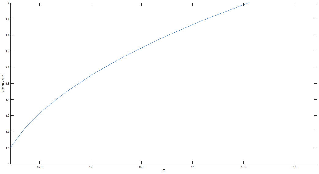
Figure 1 indicates that the equity warrant value is an increasing function with respect to the time T when other parameters remain unchanged. This is because the longer the time, the more likely it is to be executed and the higher the price of the equity warrant. This law is common sense in the financial markets.

Example 1.

Let $N=50, T-t=3, M=100, k=1, S_t=100, {\sigma }_s=0.04, J=50, r=0.04, \mu =0.02$. Then, based on approximations $V_t\approx N{S}_t$ and $\sigma \approx {\sigma }_s$, the value of the equity warrant is

$$\begin{array}{c}\hfill f_w=16.83.\end{array}$$

5. Conclusions

The value of an equity warrant was examined within the structure of uncertainty probability in this paper. In light of the supposition that the firm’s worth follows an uncertain differential equation, the model of equity warrants for an uncertain stock model was inferred with the strategy for uncertain analysis.

References

- Black, F.; Scholes, M. The pricing of options and corporate liabilities. J. Political Econ. 1973, 81, 637–654. [Google Scholar] [CrossRef] [Green Version]
- Liu, B. Uncertainty theory. In Uncertainty Theory; Springer: Berlin/Heidelberg, Germany, 2007; pp. 205–234. [Google Scholar]
- Liu, B. Some research problems in uncertainty theory. J. Uncertain Syst. 2009, 3, 3–10. [Google Scholar]
- Chen, X. American option pricing formula for uncertain financial market. Int. J. Oper. Res. 2011, 8, 32–37. [Google Scholar]
- Chen, X.; Gao, J. Uncertain term structure model of interest rate. Soft Comput. 2013, 17, 597–604. [Google Scholar] [CrossRef]
- Chen, X.; Liu, Y.; Ralescu, D.A. Uncertain stock model with periodic dividends. Fuzzy Optim. Decis. Mak. 2013, 12, 111–123. [Google Scholar] [CrossRef]
- Xiao, W.; Zhang, W.; Xu, W.; Zhang, X. The valuation of equity warrants in a fractional Brownian environment. Phys. A Stat. Mech. Appl. 2012, 391, 1742–1752. [Google Scholar] [CrossRef]
- Kremer, J.W.; Roenfeldt, R.L. Warrant pricing: Jump-diffusion vs. Black–Scholes. J. Financ. Quant. Anal. 1993, 28, 255–272. [Google Scholar] [CrossRef]
- Zhang, W.G.; Xiao, W.L.; He, C.X. Equity warrants pricing model under Fractional Brownian motion and an empirical study. Expert Syst. Appl. 2009, 36, 3056–3065. [Google Scholar] [CrossRef]
- Tversky, A.; Kahneman, D. Advances in prospect theory: Cumulative representation of uncertainty. J. Risk Uncertain. 1992, 5, 297–323. [Google Scholar] [CrossRef]
- Tversky, A.; Kahneman, D. Advances in prospect theory: Cumulative representation of uncertainty. In Readings in Formal Epistemology; Springer: Cham, Switzerland, 2016; pp. 493–519. [Google Scholar]
- Yao, K. No-arbitrage determinant theorems on mean-reverting stock model in uncertain market. Knowl. Based Syst. 2012, 35, 259–263. [Google Scholar] [CrossRef]
- Zhang, Z.; Liu, W.; Sheng, Y. Valuation of power option for uncertain financial market. Appl. Math. Comput. 2016, 286, 257–264. [Google Scholar] [CrossRef]
- Zhang, Z.; Liu, W.; Ding, J. Valuation of stock loan under uncertain environment. Soft Comput. 2017, 22, 5663–5669. [Google Scholar] [CrossRef]
- Liu, B. Fuzzy process, hybrid process and uncertain process. J. Uncertain Syst. 2008, 2, 3–16. [Google Scholar]
- Liu, B. Uncertaint Theory: A Branch of Mathematics for Modeling Human Uncertainty; Springer: Berlin/Heidelberg, Germany, 2010. [Google Scholar]
- Chen, X.; Ralescu, D.A. Liu process and uncertain calculus. J. Uncertain. Anal. Appl. 2013, 1, 3. [Google Scholar] [CrossRef] [Green Version]
- Yao, K.; Chen, X. A numerical method for solving uncertain differential equations. J. Intell. Fuzzy Syst. 2013, 25, 825–832. [Google Scholar] [CrossRef]
Figure 1.
Equity warrant price with respect to time.
Publisher’s Note: MDPI stays neutral with regard to jurisdictional claims in published maps and institutional affiliations. |
© 2022 by the author. Licensee MDPI, Basel, Switzerland. This article is an open access article distributed under the terms and conditions of the Creative Commons Attribution (CC BY) license (https://creativecommons.org/licenses/by/4.0/).
Share and Cite
MDPI and ACS Style
Shokrollahi, F. Equity Warrants Pricing Formula for Uncertain Financial Market. Math. Comput. Appl. 2022, 27, 18. https://doi.org/10.3390/mca27020018
AMA Style
Shokrollahi F. Equity Warrants Pricing Formula for Uncertain Financial Market. Mathematical and Computational Applications. 2022; 27(2):18. https://doi.org/10.3390/mca27020018
Chicago/Turabian StyleShokrollahi, Foad. 2022. "Equity Warrants Pricing Formula for Uncertain Financial Market" Mathematical and Computational Applications 27, no. 2: 18. https://doi.org/10.3390/mca27020018