AutoML for Feature Selection and Model Tuning Applied to Fault Severity Diagnosis in Spur Gearboxes

Abstract

Gearboxes are widely used in industrial processes as mechanical power transmission systems. Then, gearbox failures can affect other parts of the system and produce economic loss. The early detection of the possible failure modes and their severity assessment in such devices is an important field of research. Data-driven approaches usually require an exhaustive development of pipelines including models’ parameter optimization and feature selection. This paper takes advantage of the recent Auto Machine Learning (AutoML) tools to propose proper feature and model selection for three failure modes under different severity levels: broken tooth, pitting and crack. The performance of 64 statistical condition indicators (SCI) extracted from vibration signals under the three failure modes were analyzed by two AutoML systems, namely the H2O Driverless AI platform and TPOT, both of which include feature engineering and feature selection mechanisms. In both cases, the systems converged to different types of decision tree methods, with ensembles of XGBoost models preferred by H2O while TPOT generated different types of stacked models. The models produced by both systems achieved very high, and practically equivalent, performances on all problems. Both AutoML systems converged to pipelines that focus on very similar subsets of features across all problems, indicating that several problems in this domain can be solved by a rather small set of 10 common features, with accuracy up to 90%. This latter result is important in the research of useful feature selection for gearbox fault diagnosis.

1. Introduction

Gearboxes are crucial devices in industrial processes, as they play an important role in power transmission. Then, fault detection and diagnosis in such devices are attracting growing interest in researches, with focus on fault severity assessment. In particular, when a fault is starting, the first stages of the failure mode are not easy to detect, in most cases, and the incipient fault is not advised until reaching severe stages that can cause damages to other devices, decrease the performance of the process, and produce economical losses [1,2].

Vibration signal is one of the most informative signals commonly used to determine the health condition of rotating machines [3]. Once a vibration signal is available, data-driven approaches can offer signal processing techniques to tackle the problem of fault detection and diagnosis by identifying certain signal characteristics in time, frequency or time-frequency domains, as proposed in [4] for gearboxes.

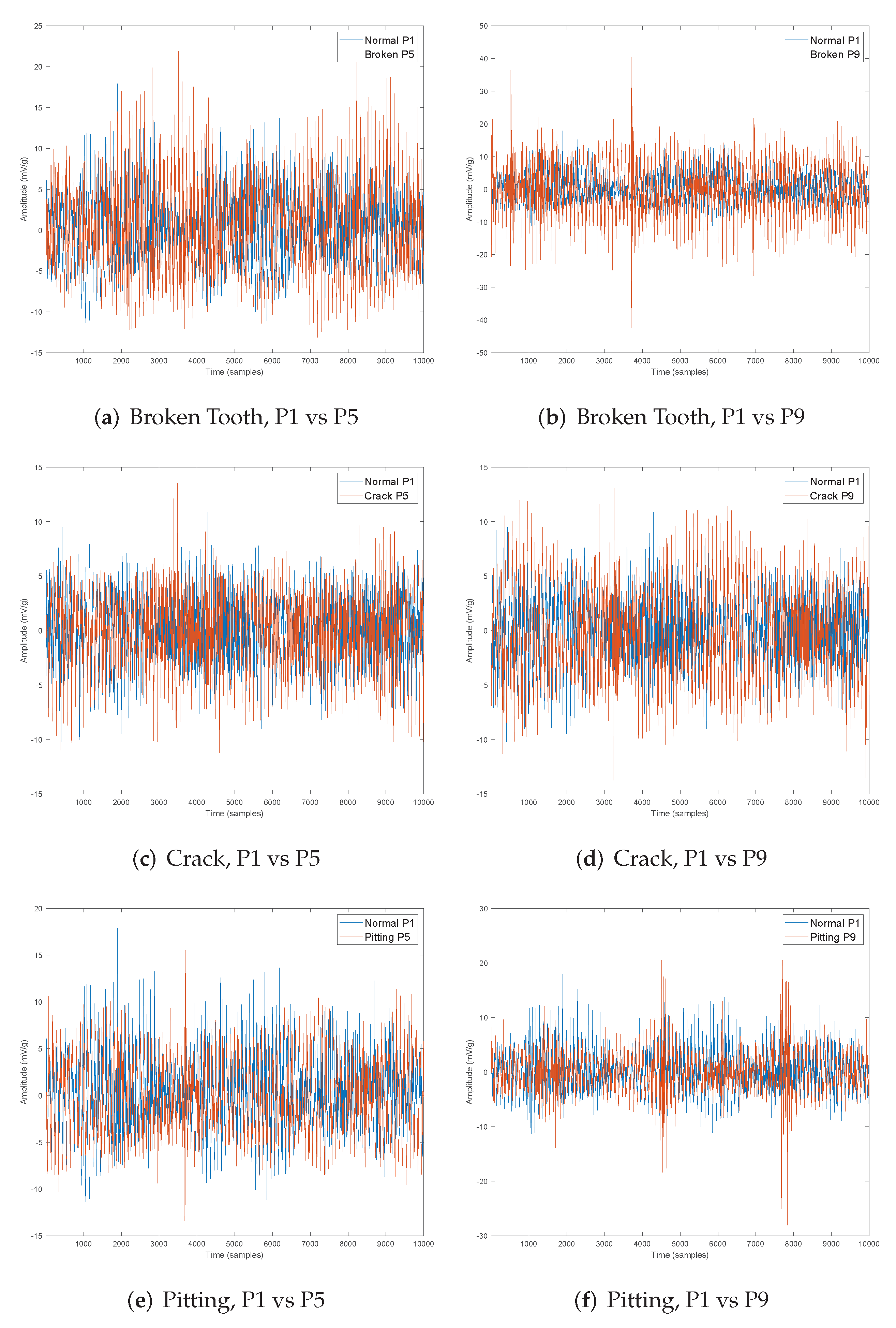
Particularly, gearboxes exhibit nonlinear and chaotic behavior [5], and these characteristics are enhanced in the presence of faults [6,7,8]. Then, the identification of informative characteristics in the vibration signal produced by faulty conditions is not easy to accomplish in gearboxes by using standard signal processing, and usually requires expert knowledge. Additionally, previous studies have visually shown that the vibration signal behavior is non-monotonic to the fault severity increment in helical gearboxes [9,10]; that is, the signal amplitude does not increase with the fault. Under this scenario, Machine Learning (ML) approaches can address properly the task of fault detection and diagnosis. Moreover, signal processing permits different characterization of the vibration signal useful for the application of ML-based approaches providing high-performance solutions, commonly being the supervised fault classification.

ML-based classifiers using the k-nearest neighbor method (KNN) [11,12,13,14], artificial neural networks (ANN) [15,16,17,18] and support vector machines (SVM) [19,20,21,22,23], are frequently developed to propose fault classification models. Random Forest (RF) and Decision Trees (DT) are also reported as fault classifiers for gearboxes because of their powerful performance in cases where only a few samples are available and high dimensional feature spaces [24,25,26,27,28].

The performance of a conventional ML-based fault classification model is highly dependent on the input feature quality, avoiding the well-known curse of dimensionality, and the selection of the best classification model. Particularly, feature selection is a stage that must be carefully accomplished after features extraction is performed on the vibration signal. Statistical condition indicators (SCI) serve as features extracted from the vibration signal in the time domain, some of them being closely related to the vibration analysis such as the root-mean-square, standard deviation, kurtosis, skewness, among others [29]. Other features are related to the biomedical field to analyze surface electromyography signals [30,31]. The availability of a large set of features makes both feature selection or the mining for new features a process that is not easily generalized.

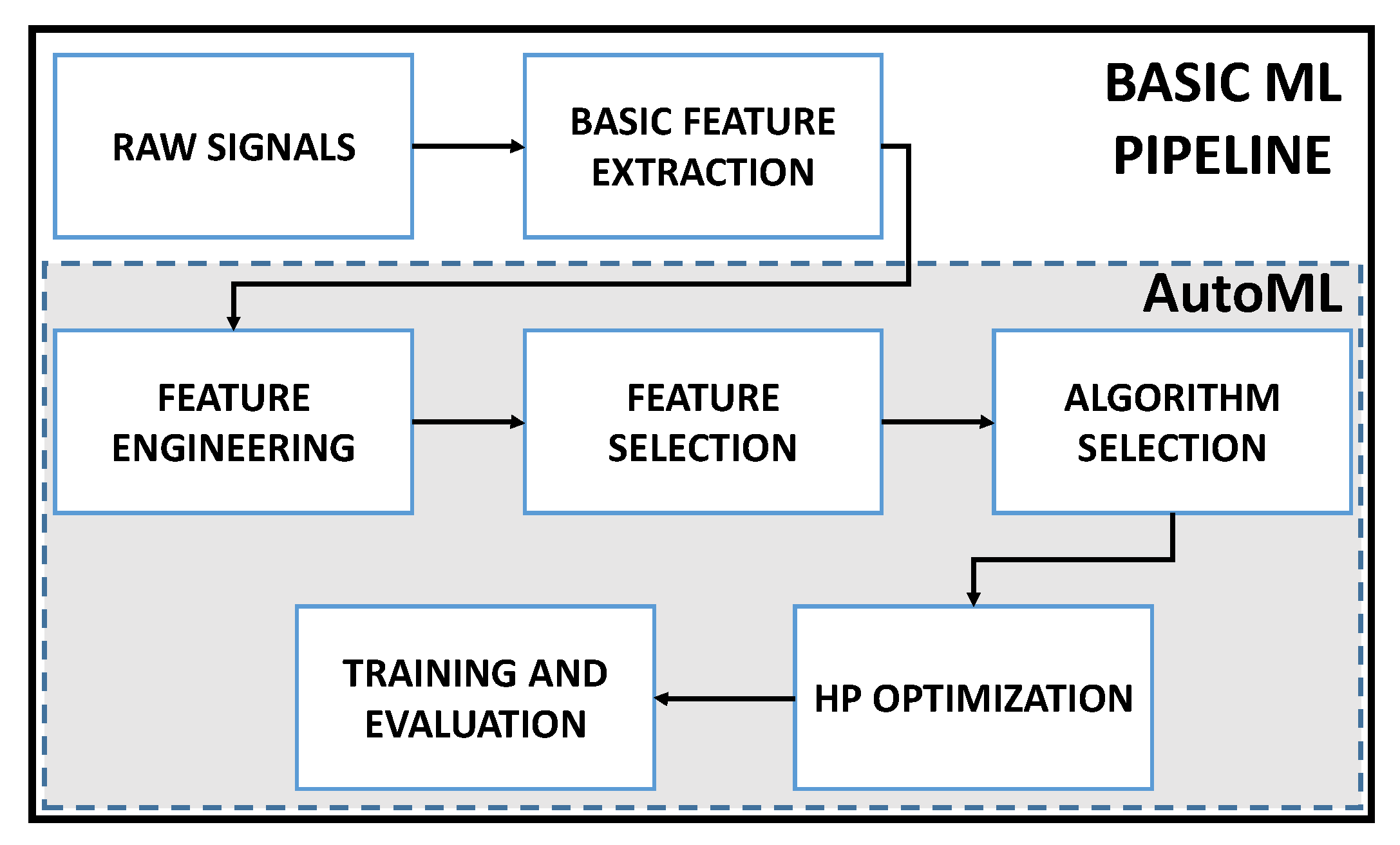
Although the recent applications of Deep Learning (DL) models to fuse the stages of feature extraction and selection are being widely reported [9,32,33,34,35,36,37,38], the selection of fault-related features like SCI extracted from the raw vibration signal is still a field of interest, mainly due to the easy understanding of such SCI. Moreover, the necessity of developing the whole ML pipeline, including not only feature engineering and selection but also classification model selection, hyperparameter optimization and validation, is currently a challenge in ML system development, called Automated Machine Learning (AutoML) [39,40].

According to the case study and the related dataset, for example, fault classification of gearboxes under different failure mode severity or multi-fault scenarios, where different failure modes are combined, the ML-based approach requires the development of a new pipeline for each scenario, that is, feature engineering and model adjustment. In most cases, this process requires exhaustive training plans, including greedy searching on feature and parameter spaces which demands computational efforts and optimization algorithms to obtain a proper classification model as mentioned previously. This is why, the development of ML pipelines automatically is nowadays highly required in practical problems associated to high dimensional feature spaces and complex model requirements. The evaluation of the different computational tools providing this support is well received by the ML-based engineering applications community in helping to choose the proper model.

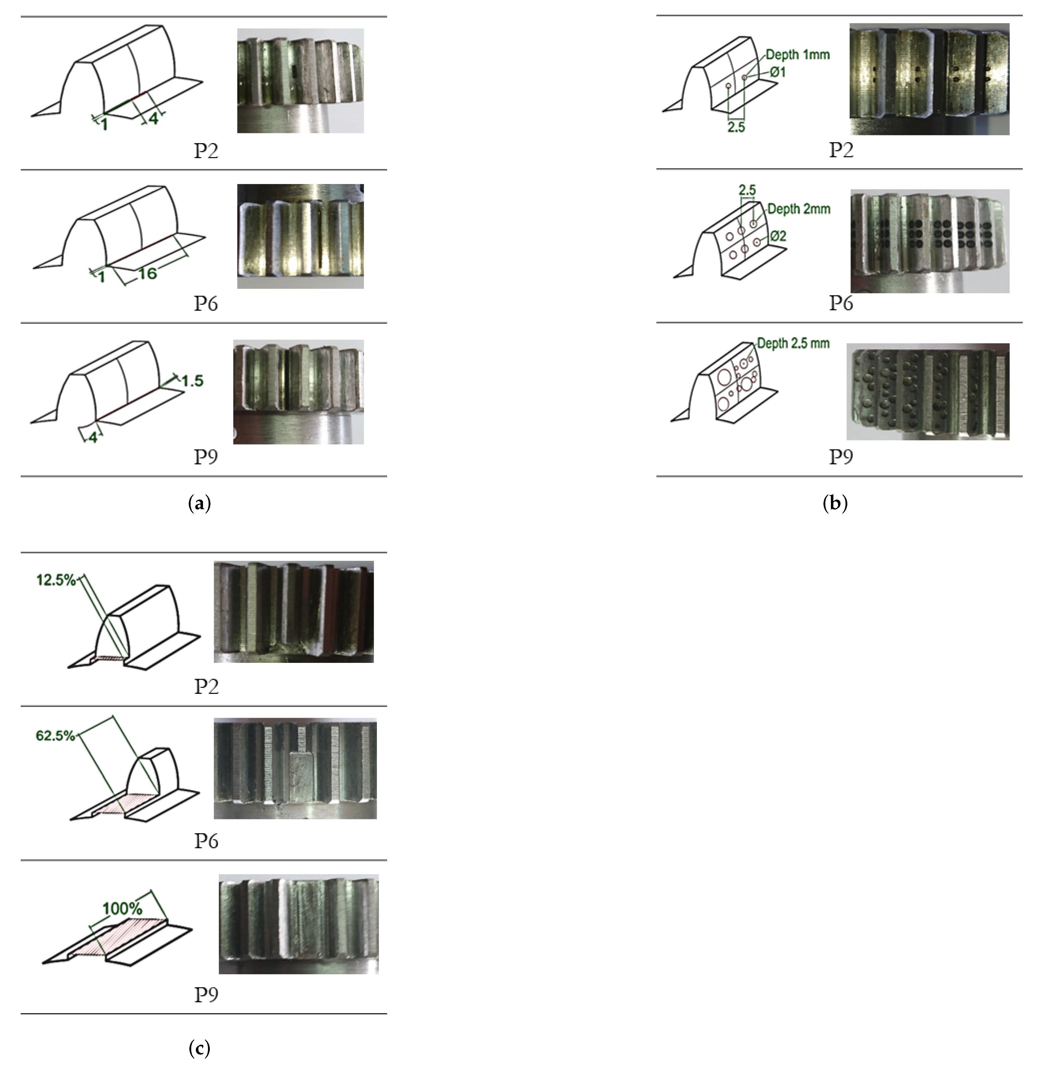
To face the automated development of ML pipelines systematically, this paper presents the application of two AutoML systems for fault severity classification, with evaluation and comparison from an empirical perspective. Particularly, the paper is focused on the feature selection stage, including feature engineering over SCI extracted from vibration signals related to the fault severity of three failure modes in gears, which are pitting, crack and broken tooth. In the following, SCI are named statistical features or features. The application of AutoML in the field of Prognosis and Health Management (PHM) is a more difficult challenge as the industrial equipment, particularly rotating machines, usually work under complex and time varying conditions of load and speed. Then, new contributions in this field are required.

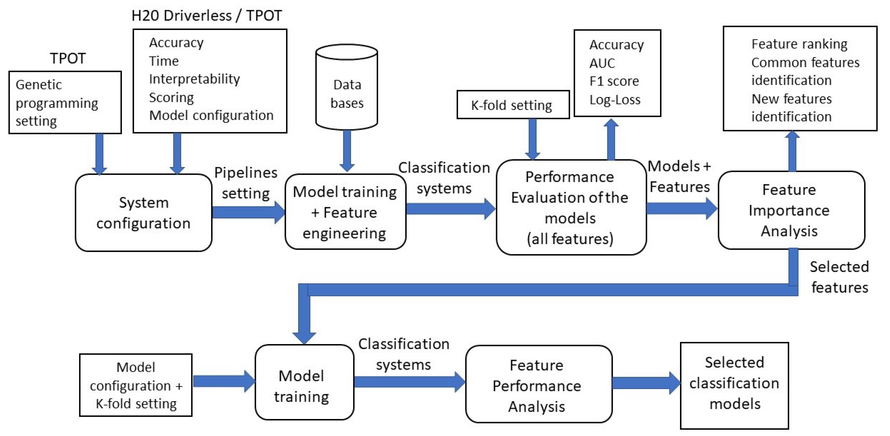
The goal is the comparison of the informative capability between the original statistical features, through the performance evaluation of the ML classifiers proposed by the AutoML systems. The experimental framework uses the software tools H2O Driverless AI which is equipped with evolutionary algorithms to perform feature engineering and selection, and TPOT, which also uses an evolutionary search to build tree-based ML pipelines. Both tools are relatively simple and straightforward to use, offering basic and intuitive configurations for generating different types of pipelines using state-of-the-art techniques and implementations.

Results of the evaluation and comparison between H2O DAI and TPOT show that both platforms select common features regardless of the selected model. For some failure modes, TPOT reduces the feature space but increase it in others. Moreover, accuracy when using the whole feature space, without feature selection, remains very close for the pipelines created by both platforms. Regarding H2O DAI, the informative capability of ten time-domain vibration signal-related statistical features is highlighted, which are enough to obtain proper classification performance.

Moreover, not only are the best features identified for each failure mode, but a common set of features reports proper performance to classify all the failure modes. This is an important contribution in the field of fault severity classification in gearboxes, for which the search for a common set of features for several failure modes in the same machine are still under research.

The rest of the paper is organized as follows. Section 2 presents the background about the AutoML as an emerging area in ML, and the description of the failure modes in gearboxes under study in this paper. Section 3 discusses the previous works regarding the feature analysis for fault severity assessment in gearboxes by using vibration signals mainly, and recent applications of AutoML on this domain. 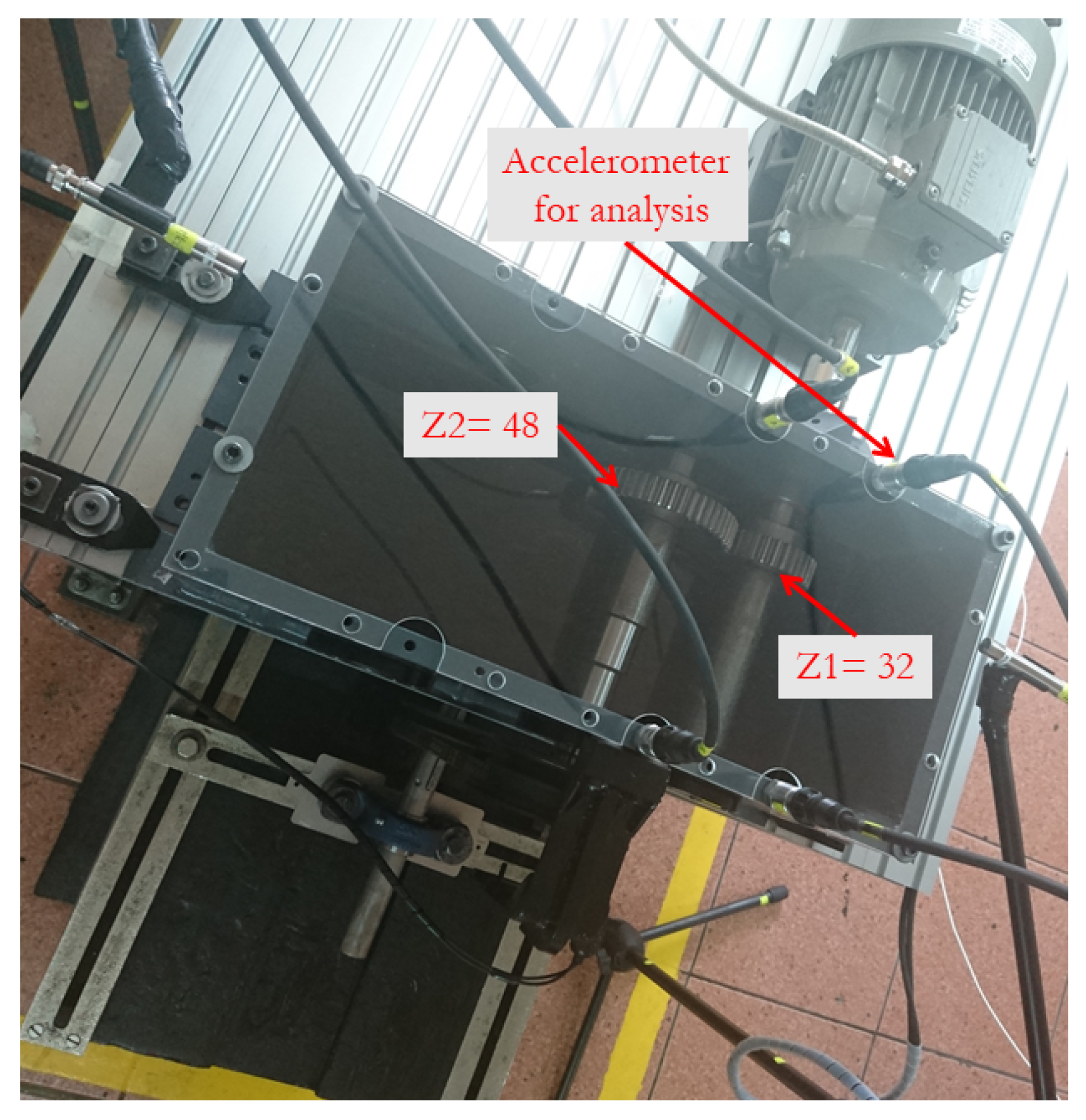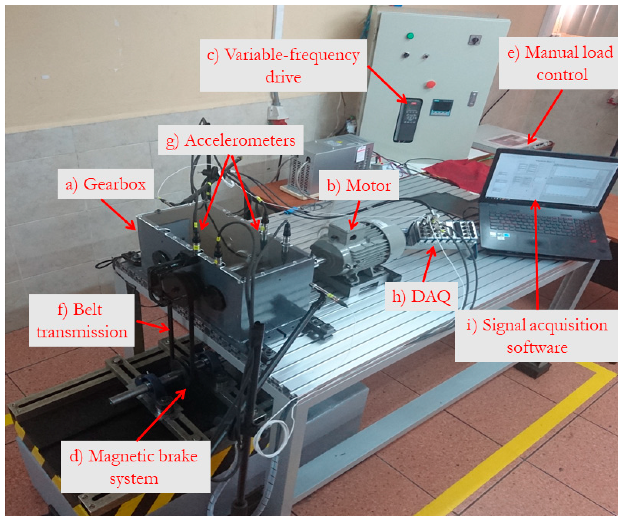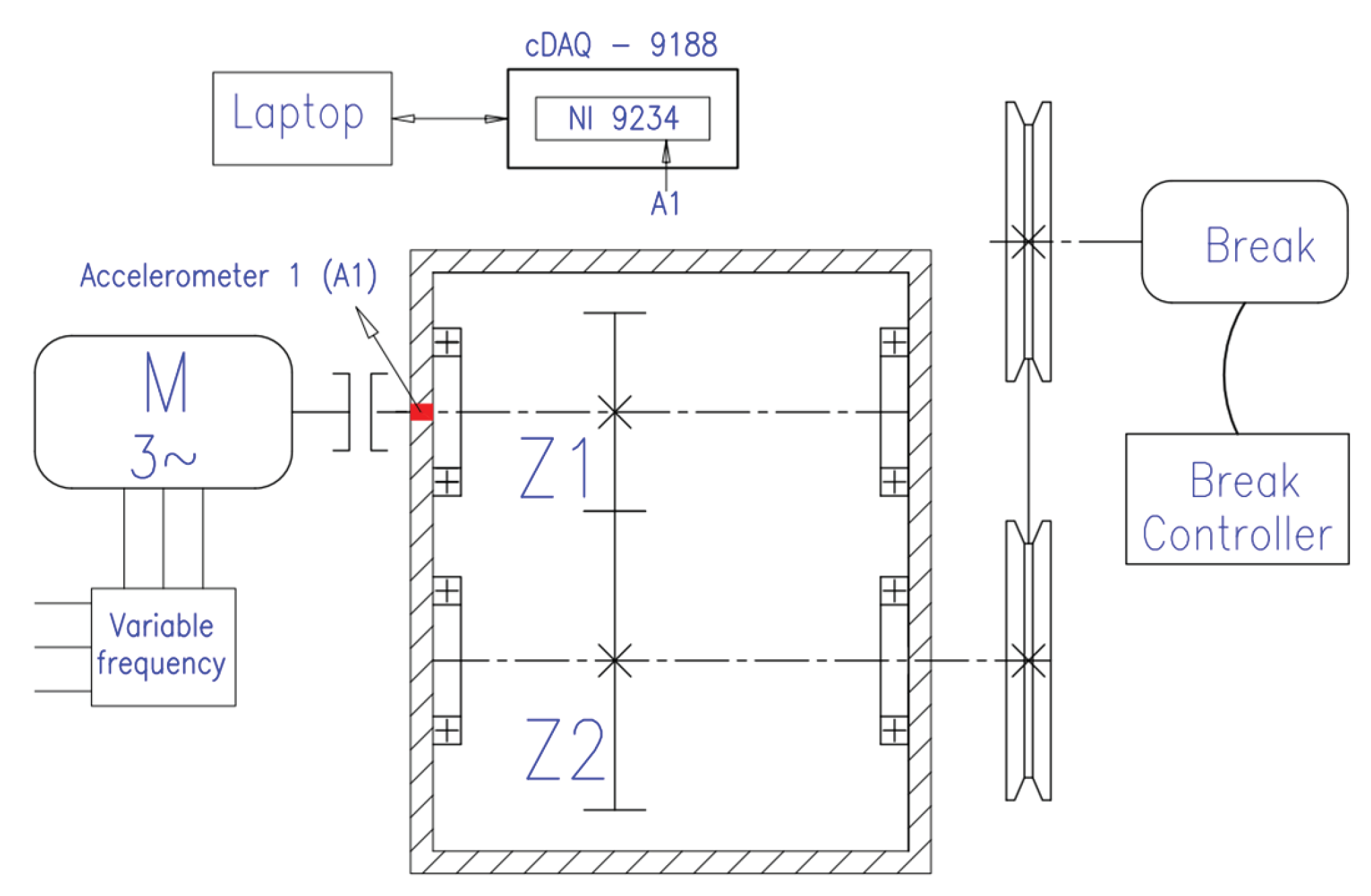Section 4 describes the test bed of the different cases study, the collection of the data set for each case and the corpus generations. Section 5 details the experimental framework and results by using the AutoML software H2O Driverless AI. Section 6 is devoted to the discussion, and finally Section 7 summarizes and concludes the paper.

2. Background

This paper presents an analysis of the applicability of AutoML in the automatic diagnosis of faults in rotating machinery, namely industrial gearboxes. Therefore, this section is intended to provide an overview of both domains, with the former covered in Section 2.1 and the latter discussed in Section 2.2.

2.1. Overview of AutoML

ML is everywhere now, with successful applications in diverse domains such as automatic programming [41] and the prediction of complex chemical processes [42], and the list of examples grows every day. This success, however, has created the need to simplify and accelerate the development of problem-specific ML deployments. Among the different strategies being taken, two paradigms are particularly promising: Transfer Learning [43,44,45] and AutoML [39,40,46,47,48,49,50,51]. The former entails using a model generated on a source task to solve a target task, simplifying learning on the target and making it more efficient. The latter, on the other hand, employs a search process to discover large model architectures [49,50,51] or to automatically derive complete ML pipelines [46,47,48]. Moreover, recent techniques are even hybridizing both methods for the construction of Deep Learning models [52].

While Transfer Learning opens up a wide range of possibilities in the domain of interest of the present work, such questions are left for future research. The focus of this paper is on AutoML. To understand AutoML, it is first necessary to review what a ML pipeline consists of. While different problems might require slight variations of the general case, a typical ML pipeline includes: (1) Feature Engineering; (2) Feature Selection; (3) Model/Algorithm selection; (4) Hyper-parameter optimization; and, finally, (5) Training and Evaluation [39,40]. In fact, some AutoML systems even facilitate model deployment for real-world use [48]. Each of the stages in a ML pipeline is a research area in and of itself, characterized by large combinatorial search spaces and highly complex and non-linear interactions. However, in general, it is not possible to determine the optimal approach for each stage based on the description or data of a particular ML task, much less the optimal configuration of a complete pipeline.

The general goal of AutoML is to simplify the design process of a ML pipeline, by automatically determining how to instantiate a ML pipeline based on a problem’s training data and a user-defined objective or scoring function. A general ML pipeline is presented in Figure 1, highlighting the elements that are usually addressed by an AutoML system. One of the most widely used variants of AutoML is Neural Architecture Search (NAS), which deals with the automated design of neural networks with a search process. While NAS has a long history [53,54], it has recently had a resurgence thanks to the intrinsic difficulty of developing Deep Neural Networks manually [49,50,51]. However, NAS is very specific to Deep Networks, focusing primarily on the Model/Algorithm selection part of the ML pipeline. The most ambitious version of AutoML are systems that cover most of the elements of the ML pipeline. Such systems work under the assumption that it is necessary to consider the interactions of all the stages in a ML pipeline; that is, an optimal pipeline will exhibit synergy among most, if not all, of the stages. To do so, it is necessary to solve a complex optimization problem, which requires performing a search within all possible ML pipelines. Given the complexity of such a search space, this type of AutoML systems often employ heuristic or meta-heuristic algorithms, such as Evolutionary Algorithms (EAs) [55].

Two such AutoML systems are TPOT [47] and H2O Driverless AI [48], with the former being an open-source academic software and the latter a commercial product specifically designed for industrial use (Driverless AI by H2O also offers academic versions of the software). TPOT is built on top of Scikit-learn [56], and while H2O is not, both share many of the underlying ML algorithms. TPOT uses genetic programming (GP), a form of EA, such that ML pipelines are coded using variable size tree structures. GP is the main search procedure in TPOT, indeed it can be seen as a basic GP system with a highly specialized primitive set and search space [55]. H2O Driverless AI, on the other hand, also uses EAs to perform Feature Engineering and Feature Selection, a task for which EAs are known to produce good results in difficult ML problems [45]. However, it employs a wider variety of mechanisms to generate the final pipeline, including Bayesian optimization for hyperparameter tuning and a large set of predefined engineered features from which the system can extend a problems feature space. In this work, we evaluate both systems to perform our experimental evaluation of AutoML because of their general simplicity and straightforward usage, where the user only needs to set very basic and intuitive configurations. Such is the goal of an AutoML system, to simplify the design process of a ML pipeline. Finally, it is important to highlight that the goal of this work is not specifically to compare the systems, even though their relative performances are contrasted. Our approach is to leverage the information produced by the ML pipelines produced by each system to better understand the feature selection problem in the domain of fault diagnosis in gearboxes, helped by this kind of AutoML systems.

2.2. Faults in Gearboxes

A gear is a toothed wheel usually attached to a rotating shaft. In a gear train, the teeth of one gear engage the teeth on the other gear. Gears and gear trains are important mechanical power transmission devices in industrial applications to produce speed and torque conversions from a rotating power source to another device. Gearboxes may work under constant or varying operation conditions of load and speed. According to the assembly of gear wheels, gear trains can be classified as a simple gear train, compound gear train, reverted gear train and planetary gear train [57]. In this work, the experimental test bed is a simple gear train assembled as a one-stage spur gearbox, with a number of teeth, Z1 and Z2, as shown in Figure 2.

In heavy machinery, complex multistage gearboxes are used and the interaction of the gearbox elements with the working environment can drive the gears to faults that may cause significant economic losses. For that reason, fault diagnosis in gears has been the subject of intensive research [57].

One of the most dangerous damages in gears is the crack at the tooth root, that is caused because of significant changes in tooth stiffness [58]. A physical simulation of a man-made crack is shown in Figure 3a, where a different length and depth of crack throughout the base of the tooth were implemented. Tooth pitting is another common failure mode of a gearbox, which can appear at several levels according to pitted areas: slight micro pitting, macro pitting, macro pitting over 50%–100% of the gear tooth surface, and macro pitting over all the gear tooth surface [59]. Tooth pits can be simulated like circles of different diameter, depth and several number of holes over the tooth surface. A physical simulation of man-made pitting is shown in Figure 3b, where pits with different diameter and depth were implemented. Finally, another important research topic is the analysis of the effect of a broken tooth on the gearbox vibration, which is caused by an excessive impact load or unstable load. Under this fault, the size of the contact surface between the meshing teeth is decreased. In addition, the tooth becomes shorter and the contact length along the in volute profile of the damaged tooth is also decreased [60]. A physical simulation of the man-made broken tooth is shown in Figure 3c, where a different percentage of tooth loss was implemented. The simulated physical failure modes were implemented at the Vibrations Laboratory of the Universidad Politécnica Salesiana (UPS-Ecuador), and they are used in this work for generating the dataset of vibration signals.

3. Previous Work

Fault severity assessment in gears by using ML has been widely reported. This section is devoted to approaches using feature extraction by calculating statistical features, and focused on the problem of feature selection, and also recent approaches using artificial features extracted from DL models.

In [12], the identification of five different gear crack levels is performed by using features obtained from Wavelet Packet Decomposition (WPD). The first set of features is composed by 620 statistical features calculated from the wavelet coefficients at different levels, which are then reduced to seven significant principal components. KNN is used as a classifier and compared to other statistical models such as linear discriminant analysis, quadratic discriminant analysis, classification and regression trees, and naive Bayes classifier. Another approach to crack fault level identification is discussed in [13] by considering 25 features extracted from the time and frequency domains. A two-stage feature selection and weighting technique via Euclidean distance evaluation is proposed to select sensitive features and to weigh the selected features according to their sensitivity to each fault level. The Weighted K-Nearest Neighbor (WKNN) classifier is adopted to identify three gear crack levels under different loads and motor speeds.

Four different crack levels are detected in [61] by using statistical features and decision trees (DT). Similar work using DT and ARMA feature extraction from the vibration signals is presented in [62]. Ordinal rough approximation operators based on fuzzy covering and feature selection algorithms for ordinal classification are proposed in [63] for gear crack level identification. Finally, a DL approach using a Long Short-Term Memory (LSTM) based recurrent neural network is discussed in [64], to detect tooth crack growth at different stages, where the vibration signal is the input to the LSTM network. The LSTM prediction error is used as a measure of fault severity.

The detection of localized pitting damages in a worm gearbox by a vibration visualization method and ANNs is presented in [18]. Twelve statistical features are calculated from vibration signals in time and frequency domains for multi-class recognition, where each class is related to a severity level. In [29], a pitting severity assessment is tackled with supervised learning using an SVM-based ranking model that learns the ordinal information contained in the dataset. Thirty-four statistical features were calculated from vibration signals in the time and frequency domain, among others specifically designed for gearbox damage diagnosis. Three levels of damage were estimated. The approach in [65] uses Stacked Auto Encoders (SAE) for unsupervised feature extraction, feature reduction based on QR decomposition is then applied on the feature matrix provided by the SAE to obtain low dimensional data feeding an unsupervised K-means clustering.

Fault severity in broken tooth is also tackled by different approaches. The approach in [9] introduces Stacked Convolutional Autoencoders (SCAE) together with a Deep Convolutional Neural Network (DCNN) as a method for unsupervised hierarchical feature extraction for fault severity assessment in a helical gearbox. In that proposal, statistical features are not extracted, but the artificial ones are provided by the DCNN after training with initialization parameters given by an SCAE. These features feed a multilayer perceptron for classification. Another approach is provided in [38], where artificial features are provided by a CNN. The spectrogram of the vibration signal is used as the input to the CNN, the output of the last convolutional layer is connected to one softmax layer and finally, these outputs feed an SVM-based decision layer. An approach based on fuzzy transition is developed in [10] to predict the broken tooth severity in helical gearboxes. This is accomplished by two steps: a set of statistical features extracted from the vibrations signal are uses as input for a static fuzzy model to compute the weights of fuzzy transitions (WFT), and then a dynamic equation using WFT predicts the next degradation state of the rotating device. All the previous works focus on the same dataset related to ten severity damages of broken tooth in helical gearboxes.

Research on AutoML arises as a way to face the challenge of automating the Combined Algorithm Selection and Hyper-parameter tuning, called CASH by [66], and recent applications can be found. The review in [67] tackles the use of AutoML for developing smart devices to obtain auto generated embedded code ready to test and execute. An Automated Hyperparameter Search-Based Deep Learning Model for Highway Traffic Prediction is performed by AutoML in [68]. In the field of process monitoring, ref. [69] uses AutoML to optimize the parameters of a soft-sensor for monitoring the lysine fermentation process. The authors in [70] propose in the future research that the AutoML approach could be used for parameter optimization of a Variational Auto Encoder for nonlinear process monitoring.

However, ML-based fault diagnosis has just started to be analyzed under this approach with only a few works in the field of fault diagnosis for rotating machines. In [71] an approach using the Google DeepMind Team method called Neural Architecture Search (NAS) with reinforcement learning is proposed, as an AutoML tool for the automated search of a multiscale cascade CNN applied to the fault diagnosis of the gearbox data set of the PHM 2009 Data Challenge. In particular, two problems were addressed: fault detection and fault severity classification. Inspired by the NAS method, in [72] a neural network architecture automatic search method based on reinforcement learning is applied to rolling bearing fault diagnosis for two cases studies: the Case Western Reserve University (CWRU) bearing dataset and the locomotive bearing data set. Inspired by AutoML approaches, a self-optimizing module is proposed in [73] to dynamically adjust the knowledge base selection and parameter setting for training an Extreme Learning Machine based on physical knowledge. The self-optimizing module was applied on the CWRU bearing dataset.

4. Case Study

This section introduces the test bed and the experimental plan to acquire the database of vibration signals from three gearbox failure modes: pitting, crack and broken tooth. Next, details of the dataset are provided.

4.1. Experimental System and Data Acquisition

The real test bed available at the Universidad Politécnica Salesiana is shown in Figure 4, where realistic conditions of load and speed can be configured. The test bed is composed by a one stage gearbox (a) with spur gears, an induction motor (b) Siemens 1LA7 096-6YA60 2Hp 1200 rpm under variable speed controlled by a variable-frequency driver (c), and a magnetic brake system (d) for manual load control (e) via belt transmission (f). The four accelerometers (g) are IMI Sensor 603C01, 100 mV/g, placed in a vertical manner. The data acquisition cards (h) are National Instrument NI 9234 and cDAQ-9188, including anti-aliasing filtering with a sample frequency of 50 KS/s and, finally, the laptop with signal acquisition software (i) developed in Labview and Matlab.

The spur gears in the gearbox are made from steel E410, with a center distance of 90 mm, the ratio Z1/Z2 of the teeth number is 32/48, the module is 2.25 and the pressure angle is 20${}^{\circ }$. The vibration signals were collected with all four accelerometers, but this work only analyses the vibration signals collected from the accelerometer (A1) placed over Z1 in a vertical manner, as shown in Figure 5. The accelerometer (A1) provides the most informative vibration signal because it is close to the motor [74].

Three failure modes are considered, namely pitting, crack and broken tooth, each one configured on the gear Z1, as detailed in

Table 1. Severity level characteristics of the three failure modes.

Label	Severity Level	Severity Level	Severity Level
	Pitting	Crack	Broken Tooth
P1	N	N	N
P2	Holes: 2	Depth: 1 mm	12.5%
	Diameter: 1 mm	Width: 1 mm
	Depth: 1 mm	Length: 4 mm
	4.1%	4.9%
P3	Holes: 2	Depth: 1mm	25.0%
	Diameter: 1.5 mm	Width: 1 mm
	Depth: 1.5 mm	Length: 8 mm
	7.3%	9.8%
P4	Holes: 4	Depth: 1 mm	37.5%
	Diameter: 1.5 mm	Width: 1 mm
	Depth: 1.5 mm	Length: 10 mm
	14.7%	12.3%
P5	Holes: 4	Depth: 1mm	50.0%
	Diameter: 2 mm	Width: 1 mm
	Depth: 2 mm	Length: 12 mm
	23.1%	14.7%
P6	Holes: 6	Depth: 1 mm	62.5%
	Diameter: 2 mm	Width: 1 mm
	Depth: 2 mm	Length: 16 mm
	34.6%	19.7%
P7	Holes: 6	Depth: 1 mm	62.5%
	Diameter: 2.5 mm	Width: 1 mm
	Depth: 2.5 mm	Length: 20 mm
	49.91%	25%
P8	Holes: 8	Depth: 2 mm	87.5%
	Diameter: 2.5 mm	Width: 1.5 mm
	Depth: 2.5 mm	Length: along the tooth
	66.5%	50.0%
P9	Holes: irregular	Depth: 4 mm	100%
	Diameter: irregular	Width: 1.5 mm
	Depth: 2.5 mm	Length: along the tooth
	83.1%	100%

. For pitting, the severity level is related to the number of holes, their diameter and depth. For cracks, the severity level is related to the depth, width and length of the crack throughout the tooth. The broken tooth was implemented as a percentage of transverse breakage on the tooth. Vibrations signals were collected for nine severity levels for each failure mode, where P1 labels the Normal (N) or healthy state, and P2 to P9 label each fault severity level. An example of the vibration signals in the time domain of each failure mode in normal conditions, severity levels P2 and P9, is presented in Figure 6. These figures show the change of the vibration amplitude, but this change is not monotonic regarding the severity level. Details about these failure modes are given in Section 2.2.

4.2. Dataset

The dataset of vibration signals were collected under the following conditions:

• The time length of each example is 10 s. Then, the signal is composed by 500,000 samples, according to the sample frequency of the DAQ card;
• The motor rotates at constant speeds of 180 rpm, 720 rpm and 960 rpm;
• The constant load was configured for no-load (0 N m), and loads generated with constant voltage application on the magnetic brake on 5 VDC (1.44 Nm) and 10 VDC (3.84 Nm);
• Each example configured under different speed and load were repeated 15 times.

Therefore, each severity level is composed by 135 examples and the whole dataset considering nine severity levels has 1215 examples. After that, 64 statistical features over the time domain of the vibration signal were extracted for each example to build the corpus matrix. The time domain offers a suitable condition indicator with easy interpretability. Some statistical features are mean, variance, standard deviation, kurtosis, skewness, energy, absolute mean, crest factor, norm entropy, Shannon entropy, sure entropy, among others. Detailed definitions of each condition indicator can be found in [29,30,31]. Then, the corpus is a 1215 × 64 matrix.

5. Experiments and Results

This section presents our general methodology to evaluate both the AutoML tools used in this paper, and the implementation details and the main findings. The methodology is presented in Figure 7, where processes (rounded squares), inputs and outputs (squares) are stated. In all of the work presented, it is important to always consider that there are three specific case studies that are analyzed, namely pitting, crack and broken tooth, each of the gearbox faults studied in this paper. The section is divided into two main subsections, each one devoted to one of the AutoML systems considered in this work.

5.1. AutoML with H2O Driverless AI

The experimental approach presented in this paper is focused on characterizing the performance of AutoML in each case study. This is done by analyzing H2O performance at different levels. First, we focus on basic generalization or testing performance, the most common approach towards evaluating ML solutions. Second, we evaluate the incidence of the Feature Engineering process on AutoML performance. It is widely understood that Feature Engineering is essential to obtain optimal performance with many ML algorithms [45]. Third, we evaluate the Feature Selection performed by AutoML, by analyzing the estimated feature importance provided by H2O and evaluating the impact that these features have on predictive accuracy. Finally, we will qualitatively compare in Section 6 the performance of the obtained AutoML results with those previously published in this domain The goal is to illustrate the differences and similarities of the AutoML pipelines relative to the standard development of ML pipelines.

5.1.1. System Configuration

H2O Driverless AI (DAI) offers an elementary user interface and control settings. In this work, we are using the version 1.6.5 of DAI, running on an IBM Power 8 HPC server, with two CPUs and 160 CPU cores, 512 GB RAM and two NVIDIA Tesla P100 GPUs with 16 GB RAM each. There are basically four elements that need to be configured by the user to perform the AutoML process, these are ( We do not cover the complete setup process, only the most relevant aspects for our study; for a detailed description please see [48] and visit the online documentation):

1.

Accuracy [1–10]: This setting controls the amount of search effort performed by the AutoML process to produce the most accurate pipeline possible, controlling the scope of the EA and the manner in which ensemble models are constructed. In all of our experiments, we set this to the highest value of 10;

2.

Time [1–10]: This setting controls the duration of the search process and allows for early stopping using heuristics when it is set to low values. In all of our experiments, we set this to the highest value of 10;

3.

Interpretability [1–10]: Guaranteeing that learned models are interpretable is one of the main open challenges in ML [75], which can be effected, for example, by model size [76]. DAI works under the assumption that model interpretability can be improved if the features used by the model are understandable to the domain expert, and if the relative number of features is kept as low as possible. This setting controls several factors, including the use of filtering features selection on the raw features, and, more importantly for our study, the amount of Feature Engineering methods used. In this work, we evaluate two extreme conditions for this setting, for each case study we perform two experiments, using a value of 1 and 10. A value of 10 filters out co-linear and uninformative feature, while also limiting the AutoML process to only use the original raw features of the problem data. On the other hand, the lower value uses all of the raw features and constructs a large set of new features using a variety of Feature Engineering methods;

4.

Scoring: Depending on the type of problem, regression or classification, DAI offers a large variety of scoring functions that are to be optimized by the underlying search performed by the AutoML system, such as Classification Accuracy or Log-Loss for classification. In this work, we choose the Area Under the Receiver Operating Characteristic Curve (AUC), where optimal performance is achieved with a value of 1, and 0 otherwise. Since all case studies are multi-class problems, this measure is computed as a micro-average of the ROC curves for each class [77].

All of the other DAI settings are left to their default values, of which one in particular merits further explanation. As mentioned before, one of the tasks that an AutoML algorithm must determine is the ML model or algorithm to use for a given dataset. DAI offers the following options: XGBoost, Generalized Linear Models, LightGBM, Follow the Regularized Leader and RuleFIt Models. After initial exploratory experiments, we observed that under all our experimental conditions, and for each case study, DAI always chose XGBoost as the learning algorithm. Therefore, XGBoost is only considered in all the experiments reported below. XGBoost is an implementation of gradient boosted decision trees, that is highly efficient, particularly on GPU-enabled systems [78]. It is widely considered to be a state-of-the-art algorithm, that consistently outperforms most other techniques on a wide variety of domains. Finally, DAI does not only consider single models, but also attempts to build ensembles of several models, an approach that often outperforms single model approaches [79]. The ensemble of XGBoost models are linearly combined to produce the final output.

5.1.2. Evaluation of AutoML Pipelines

Given the three case studies (Pitting, Crack and Broken Tooth), and the two experimental configurations (Interpretability set to 1 and Interpretability set to 10), we have a total of six sets of experimental results. DAI performs 3-fold cross validation to compute the performance scores, and presents averages of performing this process 3 times.

Table 2. Summary of experimental results for each problem (BT = Broken Tooth, Interpret = Interpretability and Acc = Accuracy). Testing performance is shown as averages and the standard deviation in parentheses. Model Size is given for the final ML pipeline found.

Configuration		Testing Performance				Model Size
Problem	Interpret.	Acc.	AUC	F1	Log-Loss	Features	Ensemble	Time
Pitting	1	0.99(0.0025)	0.99(0.0002)	0.97(0.0116)	0.09(0.0185)	177	4	19
Pitting	10	0.99(0.0021)	0.99(0.0005)	0.96(0.0009)	0.12(0.0253)	27	1	8.5
Crack	1	0.99(0.0023)	0.99(0.0001)	0.98(0.0106)	0.08(0.0176)	131	4	18.5
Crack	10	0.99(0.0015)	0.99(0.0002)	0.98(0.0007)	0.08(0.0197)	25	2	14.8
BT	1	0.98(0.0027)	0.99(0.0003)	0.95(0.0124)	0.17(0.0161)	1019	3	19.5
BT	10	0.98(0.0040)	0.99(0.0002)	0.94(0.0180)	0.17(0.0556)	15	2	14.7

summarizes the results for each experiment, focusing on the following performance metrics: Classification Accuracy, AUC, F1 Measure and Log-Loss, all of which are standard measures in the ML literature. These measures are given as averages over all test folds in the cross validation process, and the standard deviation is given in parentheses. The next two columns present the details on model size, given by the number of features used and the number of components in the final ensemble (In some cases the number of components in the final ensemble was larger than what we report in Table 2, but some models had a zero weight, so they were omitted from the final result). It is worthwhile to mention, once again, that while size is not equivalent to complexity or interpretability, in practice it often sufficiently commensurate to be used as a useful approximation [76]. The final column specifies the amount of computation time required for each experiment (in hours).

There are some notable results in Table 2. First, in terms of generalization performance, all of the ML pipelines produce very strong results. Second, the Interpretability setting does not seem to have a significant effect on performance, with almost identical results for both settings. Third, this setting does affect the number of features used and the running time of the experiments. It is clear that using an Interpretability setting of 1 does increase the number of features, in some cases quite drastically (Broken Tooth in particular), but it does not generate a similar performance increase. This phenomenon is well studied in the EA literature, and it is known as bloat [76]. While widely studied, and a variety of methods used to control it, it is obviously not addressed in this state-of-the-art AutoML system.

5.1.3. Analysis of Feature Importance

While feature engineering did not lead to substantial improvements in classification accuracy, however, the AutoML feature importance estimation and feature selection process are also evaluated.

Table 3. Feature importance computed by DAI on each problem, for each of the features used in this study. Features not on this list had a zero value in all three problems. Dark gray rows indicate that a feature was used in all three problems, light gray in two, and white in at least one.

Feature	Pitting	Crack	Broken Tooth	Average
$x_1$	1	1	1	1
$x_5$	0.07	0	0	0.02
$x_6$	0.92	0.63	0.93	0.88
$x_7$	0.52	0.77	0.20	0.49
$x_8$	0.50	0.71	0.90	0.70
$x_9$	0	0.14	0.57	0.23
$x_{10}$	0.06	0	0	0.02
$x_{11}$	0	0.64	0	0.02
$x_{12}$	0.05	0.18	0	0.07
$x_{13}$	0.51	0	0.61	0.37
$x_{15}$	0.17	0.65	0	0.27
$x_{16}$	0.14	0	0	0.04
$x_{17}$	0.09	0	0	0.03
$x_{19}$	0.51	0.38	0	0.29
$x_{20}$	0.52	0.18	0	0.23
$x_{21}$	0.11	0.30	0	0.13
$x_{22}$	0.05	0	0.97	0.34
$x_{24}$	0.25	0	0	0.08
$x_{26}$	0	0.44	0	0.14
$x_{27}$	0.63	0.70	0.52	0.61
$x_{28}$	0.06	0.72	0	0.26
$x_{30}$	0	0	0.49	0.16
$x_{33}$	0	0	0.20	0.06
$x_{35}$	0.27	0.16	0.65	0.36
$x_{39}$	0.05	0.19	0	0.08
$x_{41}$	0.52	0.65	0.94	0.70
$x_{42}$	0.27	0.19	0	0.09
$x_{45}$	0	0.62	0	0.20
$x_{54}$	0.24	0.56	0.19	0.33
$x_{58}$	0.05	0	0.55	0.20
$x_{61}$	0.39	0.68	0.22	0.43
$x_{62}$	0	0.18	0	0.06
$x_{63}$	0	0.15	0	0.05
$x_{64}$	0.05	0.77	0	0.27

presents a summary of the feature importance scores assigned by DAI to each of the features used in this study, which are given in the range of $[0,1]$, when setting $Interpretability=10$. Features that are assigned a value below $0.003$ are not used by the ML pipeline found in a particular problem, and those features with such a value in all three pipelines are omitted from the table. Notice that the number of features that meet these criteria for each problem is well below the total number of available features: 26 for pitting, 15 for Broken Tooth and 24 for crack.

Moreover, features that were used in the pipeline of all three problems (feature importance values greater than $0.003$ in all pipelines) are highlighted in gray (nine features), these are: $x_1$, $x_6$, $x_7$, $x_8$, $x_{27}$, $x_{35}$$x_{41}$, $x_{54}$, and $x_{61}$. Features that are only used in at least two of the pipelines are in light gray (12 features), and features that are used once are in white (12 features). The final column of Table 3 presents the average Feature Importance score assigned by DAI to each feature, considering the score from the pipeline obtained from each problem. These results show that there is substantial agreement in which features are informative in this domain, irrespective of the specific type of fault.

Taking into consideration the results in Table 2, there are several observations that can be made regarding feature importance and the DAI results that did employ Feature Engineering (Interpretability = 1). These results show that feature engineering produces a larger set of informative features, compared to the original set of features. For instance, we can focus on the top 50 features determined by DAI, and analyze them based on their feature importance value to characterize their statistical distribution, as summarized in

Table 4. Feature importance values for the top 50 features found for each problem by DAI.

Configuration		Feature Importance
Problem	Interpret.	Min	Max	Median	Mean	Std
Pitting	1	0.149	1	0.212	0.259	0.152
Pitting	10	0.114	1	0.183	0.233	0.147
Crack	1	0.281	1	0.414	0.462	0.180
Crack	10	0.003	1	0.052	0.166	0.248
BT	1	0.003	1	0.003	0.182	0.319
BT	10	0.003	1	0.062	0.237	0.301

(Note that for the experiments with Interpretability = 10 some features (in some cases most) did not achieve a feature importance value greater than $0.003$, and were thus omitted from the analysis in Table 3. However, since DAI does not provide the feature importance value for these features, it was considered to be equal to $0.003$ for this analysis). These results clearly show that the feature engineering process did produce a larger set of informative features, compared to the original set of raw features. We can also analyze the type of features used by DAI when setting Interpretability = 1, as summarized in

Table 5. Percentage of types of features used by DAI on each problem, based on the 50 features with the highest feature importance scores.

Problem	Original	CD	CTE	Interaction	TSVD
Pitting	48%	32%	0%	18%	2%
Broken Tooth	32%	30%	0%	36%	2%
Crack	8%	52%	4%	36%	0%

, again focusing on the top 50 features for each problem. The table summarizes the percentage of features generated by different Feature Engineering heuristics; these are:

• Original: The original features in the dataset;
• Cluster Distance (CD): Uses a subset of features to cluster the samples, and uses the distance to a specific cluster as a new feature;
• Cluster Target Encoding (CTE): Also cluster the data, but computes the average value of the target feature of each cluster as a new feature;
• Interaction: Uses feature interactions as new features, based on simple arithmetic operations, namely addition, subtraction, division, and multiplication;
• Truncated SVD (TSVD): This heuristic trains a truncated SVD model on a subset of the original features, and uses the components of the SVD matrix as new features for the problem.

It appears that the original features and the CD and Interaction heuristics produce most of the informative features used by the DAI models. However, as shown in Table 2, these features did not lead to increased performance in the studied problem instances. Suggesting, once again, that these transformations are, in fact, reducing model interpretability without notably improving model accuracy.

5.1.4. Feature Importance and Classification Performance

To better understand how classification performance depends on the number of features used, two experiments were carried out. In both, an XGBoost classifier was evaluated on each problem using an increasing number of features, starting with the feature with the highest Feature Importance value and progressively adding the next highest and so on. In the first experiment, independent feature importance lists were used, as given by the DAI pipeline for each problem. For the second experiment, a common feature importance list was implemented, using the average importance value for each feature among the three problems. The values are presented in the Average column in Table 3.

This analysis allows us to characterize how the least important features impact classification accuracy. In these experiments, an 80%/20% training/testing split was carried out. Training was carried out using a Grid Search over hyperparameter space and 10-fold cross validation. Hyperparameter optimization considered the following hyperparameters and search ranges:

• Number of estimators ($n_{est}$): The number of weak-learners used by the XGBoost classifier. The search range is $\{50,100,150,200\}$;
• Learning rate ($lr$): Size of each bootstrapping step, and it is critical to prevent overfitting. The search range is $\{0.01,0.1,0.2,0.3\}$;
• Max Depth ($d_{max}$): Maximum depth of each weak-learner, which is represented as a decision tree. The search range is $[3,10]$;
• Feature Subsampling ($SS$): Represents the fraction of features that are subsampled by a particular learner. The search range is $[0.1,0.2]$;
• Gamma ($\gamma$): A regularization term that controls when a leaf is split in a weak-learner decision tree. The search range is $\{0,0.1,0.2\}$.

For the first experiment, the feature importance values for each problem are listed in Table 3. The results on the training and test set, for each number of features, are summarized in the first column of Figure 8, which shows the classification accuracy for each problem. What it is clear is that the highest accuracy is reached by all methods with 10 to 16 features, which is significant since it is less than the number of features used by the DAI pipelines from the Pitting and Crack problems. This suggest that further feature selection, at least in these two cases, can be beneficial. It is also important to note that this experiment is using a single XGBoost classifier, instead of the ensembles suggested by the DAI pipeline, but performance is nonetheless comparable. The second column of Figure 8 shows the optimal hyperparameter values found on each problem for each number of total features used, each one normalized to the range $[0,1]$.

In the second experiment, as stated above, features were added using a common list of features based on the average feature importance values. Results are summarized in Figure 9 and several observations are pertinent when compared with the results in Figure 8. First, it is clear that performance does not decrease when using a common set of features, suggesting that the same set of features can be used to solve all three classification tasks. Second, hyperparameter optimization behaves very similar, across all problems and in both experimental setups. When using a few features, a large learning rate and deep trees are preferable, while more estimators, shallower trees and a smaller learning rate is better when using more features.

5.2. AutoML with TPOT

TPOT incorporates several similar basic elements as H2O does, which are feature transformation, feature engineering, feature selection, parameter optimization and modeling. However, it takes a different approach to do so, using a form of evolutionary search called Genetic Programming [47], and building on top of the well-known ML library Scikit-learn [56]. TPOT basically uses four types of pipeline elements, namely preprocessors, decomposition operators, feature selection and modeling. Preprocessors include various types of scaling techniques for input data, as well as basic feature engineering methods based on polynomial expansions of the input features. Decomposition operators include different forms of PCA, while feature selection techniques include recursive feature elimination (RFE) or filtering techniques such as SelectFwe, which is based on the family wise error of each feature [56]. For classification problems, modeling techniques include KNN, linear SVM, logistic regression, Gradient Boosting, Extra Tree classifiers and XGBoost, to name a few.

TPOT is configured to maximize classification accuracy as well as to minimize model complexity (given by the size of the pipeline). Since these two objectives can be potentially in conflict, TPOT employs a multi objective criteria to guide the search for the best ML pipeline for a given problem.

While TPOT does not include such a rich set of explicit feature engineering methods, it achieves the same type of results by employing stacking of models. In summary, stacking allows TOT to concatenate the output of several models in such a way that all the outputs from a particular model can be used as additional features to train another model which is further downstream in the pipeline. For instance, a Gradient Boosting model will produce m probabilistic outputs for each sample, where m is the number of classes; that is, the probability that a particular sample belongs to each class. This output vector can be concatenated with the original input features to form an extended feature set for another ML model.

5.2.1. TPOT Configuration and Results

The same datasets and cross validation procedure was used with TPOT as was done with H2O. However, the configuration of the system is notably different, with the underlying Genetic Programming algorithm requiring a set of specific hyperparameters to perform the run. For the presented experiments, we used the same configuration suggested in [47]. The average cross validation testing performance (accuracy) on each problem was: 0.99 for pitting, 0.98 for crack and 0.96 for Broken Tooth. Comparing these results with those presented in Table 2 shows that overall, the performance of the ML pipelines produced by both AutoML systems are quite similar. However, given the different approaches towards ML pipeline generation, the pipelines generated by TPOT are more heterogeneous than those produced by H2O.

TPOT Pitting Pipeline

For this problem, TPOT produced the most complex pipeline, which consisted of:

• First, an RFE feature selection step that reduced the feature space to hold the number of original features;
• A filtering of the features using SelectFwe, which left a total of 27 original features. It is of note that the number of features used in this pipeline is the same as those used by H2O on the same problem (see Table 2 for Pitting with Interpretability set to 10);
• Feature transformation by PCA, followed by a robust scaling;
• Finally, modeling was carried out by the Extra Tree classifier with 100 base learners.

TPOT Crack Pipeline

For this problem, TPOT produced the following pipeline:

• The pipeline stacked two models in this pipeline. The first model is a Multilayer Perceptron (MLP) with a learning rate of 1 and 100 hidden neurons;
• The outputs from the MLP were concatenated with the original feature set and used to train the second model, a Gradient Boosting classifier with learning rate 0.5, max depth of 7, minimum sample split of 19 and 100 base learners.

TPOT Broken Tooth Pipeline

For this problem, TPOT produced the following pipeline:

• The pipeline stacked two models in this pipeline. The first model is a Gradient Boosting classifier with learning rate 0.5, max depth of 4, minimum sample split of 10 and 100 base learners;
• The second model is a linear SVM classifier, with a squared hinge loss function, and L1 regularization.

It is noticeable that, unlike H2O, TPOT does not converge to XGBoost models, but does use a decision tree-based model in all three pipelines. Moreover, TPOT reduces the feature space on pitting, but increases the feature space with stacking on the other two problems.

5.2.2. Analysis of Feature Selection and Feature Importance

Unlike H2O, TPOT does not generate an explicit feature ranking or feature importance score, a notable and useful feature of the former method. However, it is possible to analyze the pipelines produced in each problem, and determine the relative feature importance assigned by the TPOT pipelines. In the following analysis, we will compare the feature selection and feature importance values produced by the TPOT pipelines relative to the results obtained by the H2O pipelines when using Interpretability = 10. In particular, we focus on the set of common features, those chosen in all three problems by the H2O pipelines; these are the following nine features from Table 3: $x_1$, $x_6$, $x_7$, $x_8$, $x_{27}$, $x_{35}$$x_{41}$, $x_{54}$, and $x_{61}$.

For the Pitting problem, there are two feature selection operators applied to the original data. After this filtering process, a total of 27 features were used to perform the classification. Relative to the common set of features found by H2O, seven of the nine features (77%) are also used by the TPOT pipeline in this problem, with the only exceptions being $x_8$ and $x_{27}$.

For the Crack problem, we can obtain a feature importance score from the Gradient Boosting classifier. It is important to remember that the Gradient Boosting classifier used a combination of synthetic features generated by the MLP and the original raw features. Based on this, we can rank the top 25 features used by the Gradient Boosting classifier, the same number of features used by the H2O pipeline. This ranking shows that all the top-ranked features are from the original feature set, without any of the synthetic features generated by the MLP. Moreover, among the top 25 features, the 9 common features from H2O are included (77%), with the only exceptions being $x_{35}$ and $x_{61}$.

Finally, we can perform the same analysis for the BT problem, considering the top 15 features (based once again on the H2O results). In this case, we use the relative feature importance produced by both stacked models on the original feature set, namely the Gradient Boosting and linear SVC. In this case, the overlap with the common features produced by H2O is 8 out of 9 (88%), with the only exception $x_{27}$.

These results show that, overall, both AutoML pipelines converge to a very similar set of features for all problems, clearly indicating which features are more relevant in this domain.

6. Discussion

The previous section shows the proper performance of the original time-domain condition indicators for fault severity classification with the model obtained by the AutoML systems. The results are compared to alternative ones obtained by the authors when the best set of features and classification model is obtained by manually adjusting the classification parameters and taking the individual ranking provided by the feature ranking algorithm [80,81].

In [80], the same dataset of the pitting damage was analyzed for vibration signals and a subset of 24 time-domain condition indicators. Feature selection was conducted by using Chi-square-based ranking and a KNN classifier. Results show that 6 features can provide over 95% of accuracy and 12 features offer over 96%.

The method proposed in [81] was adopted to perform feature selection by using relief-based feature ranking and tested on a RF classifier, with the same dataset used in this work. Results are show in

Table 6. Accuracy by using RF-based classifier and feature ranking with RelieF.

Number of Features	Pitting	Broken Tooth	Crack
1	0.32	0.29	0.32
2	0.56	0.52	0.55
3	0.80	0.80	0.82
4	0.88	0.89	0.93
5	0.92	0.91	0.94
6	0.92	0.93	0.95
7	0.93	0.93	0.96
8	0.92	0.94	0.97
9	0.94	0.95	0.97
10	0.93	0.96	0.96
11	0.94	0.97	0.97
12	0.95	0.97	0.97
13	0.96	0.97	0.97
14	0.96	0.97	0.97
15	0.96	0.96	0.97
16	0.96	0.96	0.97
17	0.97	0.96	0.97
18	0.96	0.97	0.97
19	0.97	0.97	0.97
20	0.97	0.97	0.96

and Figure 10.

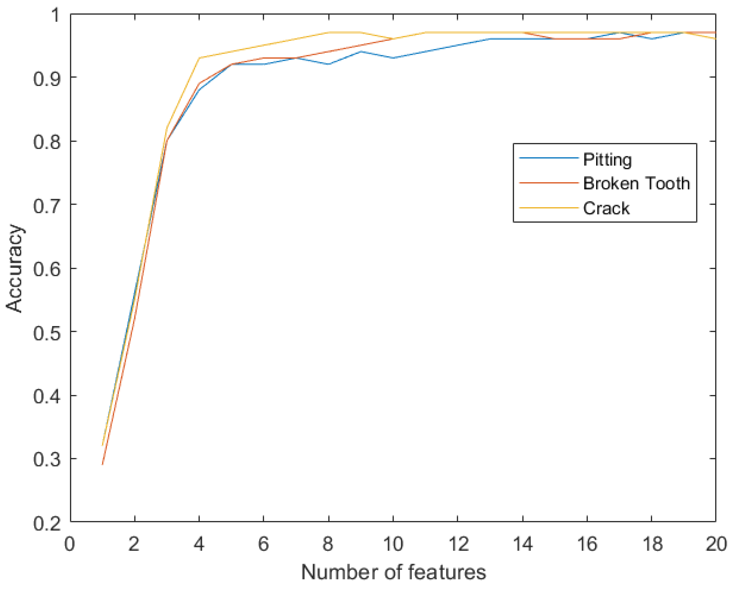
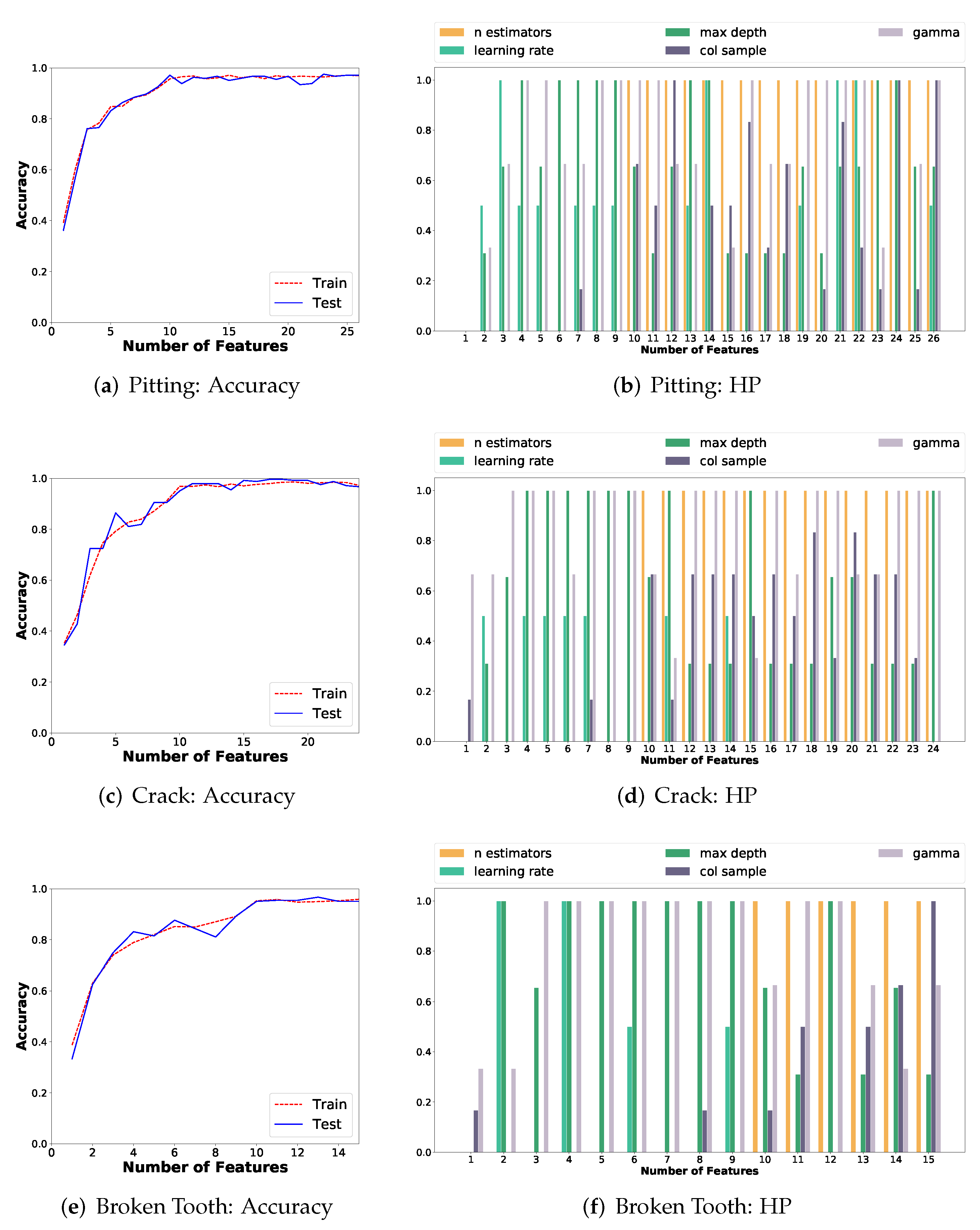
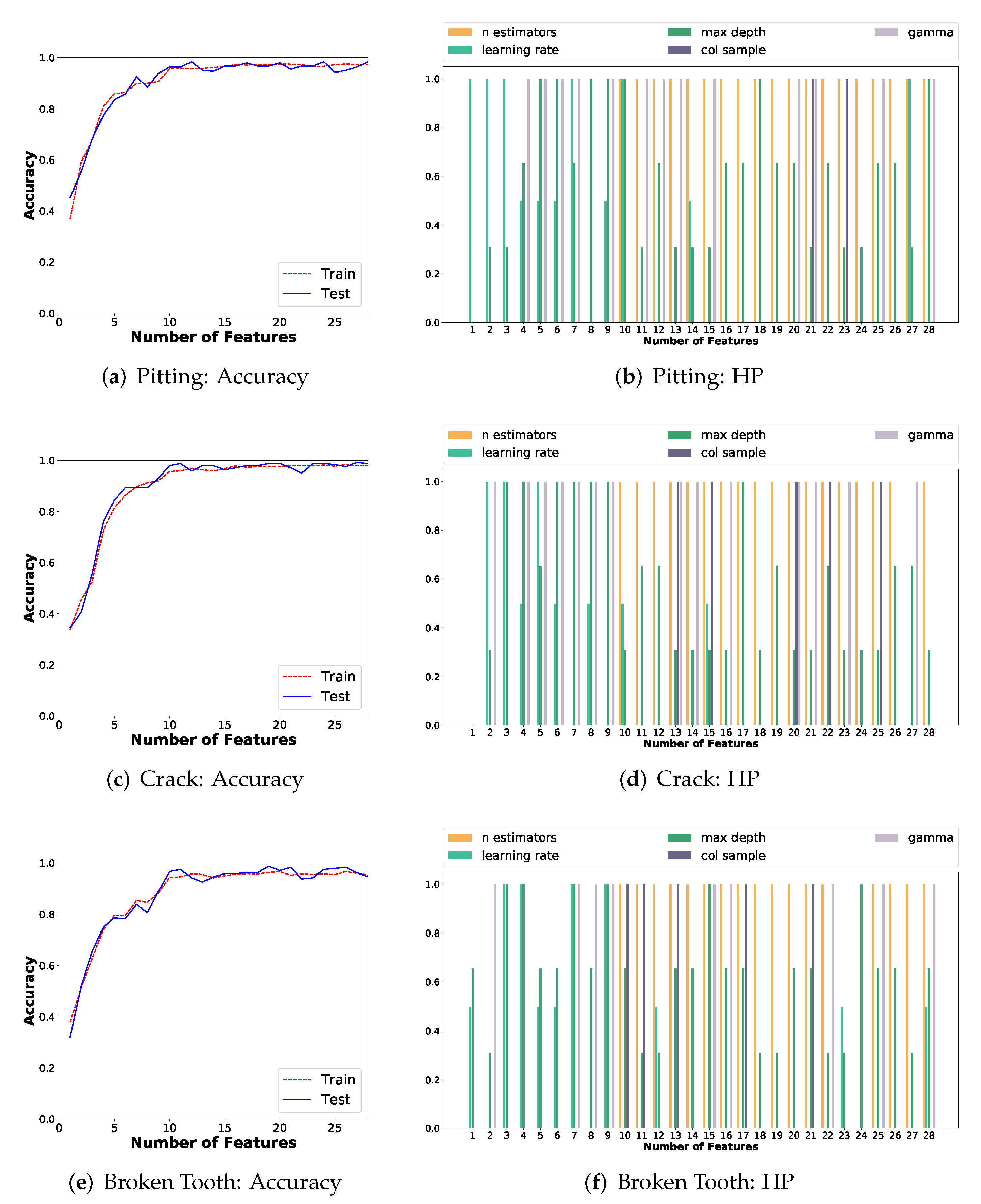
Results in Table 6 show that, for all the three failures modes, the accuracy remains above 97% with more than 13 features. By comparing to Figure 8, this trend is similar, and the accuracy is around 96% for pitting, 98% for crack, and 95% for Broken Tooth, when test examples are used. By comparing to Figure 9, when common features are used, the average accuracy over 98% is attained for pitting, 96% for crack and 97% for Broken tooth, by using over 13 features and test examples.

These results are similar for feature selection and classification using AutoML. The aggregate value of using AutoML is that the search is guided by an optimization problem, simplifying the underlying design process of the ML pipeline. However, at least on the tested problems, the overall performance of the resulting pipeline is not substantially different from those achieved by the standard pipeline design approach. On the other hand, given the simplified approach to ML development, this work was able to show that the same set of features can be used to solve three different fault diagnosis problems in gearboxes, which was previously unknown and not reported by other works in our knowledge.

7. Summary and Conclusions

This paper presents the application of two AutoML systems, H2O DAI and TPOT, for obtaining fault severity ML pipelines for spur gears under three different failures modes at different severity levels. The case study in this work is for fault severity assessment in gearboxes, treated as classification problems for three failure modes: pitting, crack and broken tooth. Fault severity assessment in gearboxes is not a trivial problem, as the gearboxes are mechanical systems with high non-linear and chaotic behaviors that usually work under changes in load and speed.

The use of AutoML to solve fault detection in gearboxes has not been previously reported in the literature, making this work the first to show the power of this approach to generate optimized ML models for this problem. Both AutoML systems are easy to use and provide both optimization modules and feature engineering modules (H2O explicitly, while TPOT mainly does this implicitly), which simplifies the design process of specialized ML pipelines.

The results and main conclusions in this paper are summarized in two ways. Regarding the general results of using AutoML in this domain:

• The setting of H2O DAI in the process of feature engineering is more explicit for the user. This is particularly useful when testing the creation of new features;
• Results of the evaluation and comparison between H2O DAI and TPOT show that both platforms select common features, regardless of the selected model by each platform. The size of the feature space used by each system varies, and neither of them is consistently more or less efficient in this regard;
• Classification accuracy when using all the features, without feature selection, remains very close for both systems, over 96%;
• The accuracy achieved by AutoML can be increased relative to a hand-tuned classification model, particularly by adjusting the feature selection technique.

Regarding the feature analysis of the generated AutoML pipelines, we can state the following:

• Time-domain statistical features are highly informative. This is verified by the fact that the feature engineering methods provided by the AutoML platforms do not substantially increase the classification accuracy of the ML pipelines. This particularity was identified because of the use of AutoML, and this discovery reduces the requirements of computing other complex features beyond the informative ones;
• Classification accuracy over 90% is obtained with 10 features, and over 95% with more than 13 features, for each failure mode, when problem-specific features are selected based on the relative feature importance. The use of AutoML permitted to set the proper number of features, and this directly improves the generalization capability of the ML model for fault diagnosis;
• Common features for all three failures modes can be selected based on average values of feature importance across all problems. These common features are highly informative as they achieve a classification accuracy over 96%. Moreover, the common set of features are ranked as highly informative for all problems by both AutoML systems. The analysis and use of the same set of features for all three failure modes has not been previously reported in the literature;
• The accuracy of the classifiers obtained by AutoML are highly competitive with the state-of-the-art in this domain, reaching 96% of accuracy and even 99% in some failure modes. For comparison, accuracy by manual design of ML pipelines has been reported of up to 97% on the same datasets. This result verifies the power of the pipelines created from AutoML.

Future works can be focused on testing other AutoML platforms, like Neural Architecture Search (NAS) developed by Google DeepMind Team, to evaluate neural network architectures or a Bayesian approach, such as Auto-Sklearn [82], for the case study presented in this work.