1. Introduction
Forest fires are currently the main menace to the sustainability of forest ecosystems and its biodiversity, in particular, and for the environment in general. This is especially true in the Mediterranean climate regions in the context of climate change scenario. The sustainability of rural landscapes is also endangered due to the effects of fire in all landscape mosaics (forest, silvo-pastoral, agro-silvo-pastoral, orchards, crops, etc.), with the consequent economic losses, and, when the urban mosaic is affected, with human and patrimonial losses [
1,
2,
3,
4]. Traditionally, research on wildfires focused on two main objectives: the prediction of the fire spreading rate and the estimation of the released heat from the flame front [
5]. Attempts to model fire behaviour mathematically go back to 1946, with Fons [
6].
Fire behaves according to three interacting physical factors: fuel availability (morphological and physiological characteristics of vegetation), weather (wind speed and direction, temperature, and relative humidity) and terrain (slope and aspect) [
7,
8]—along this article we will refer to such factors as FWT conditions. Based on the knowledge of a land patch regarding these factors, and data on the initial fire condition it’s possible to calculate an average value for the fire spreading rate [
9]. Fire models such as Rothermel’s [
10] predict fire’s local behaviour and use fuel model parameters as input. Fuel models, such as [
11,
12] and those presented by NFDRS, are sets of input parameters that describe the inherited characteristics that have been found in certain fuel types in the past. Additionally, the environmental parameters of wind, slope, and expected moisture changes can also be superimposed on these fuel models [
10].
One of the existing strategies for fire spreading mitigation is the implementation of fire-breaks. A fire-break is a gap in the vegetation and combustible material that prevents the fire from advancing. It’s a very important structure in confining the burned area as well as delaying the spread of the fire [
13,
14], thus facilitating the combat.
As a complementary effort to mitigate fire spread consequences, our goal is to establish an efficient fire-break structure, i.e., with an optimal relation between cost and effectiveness.
Due to limitations of experimental work at a large scale, our strategy consists on building a spatial multilayer network from bottom to top, focusing on understanding fire behaviour only locally and evaluating the range of its spreading at the landscape scale. In this structure, the landscape network is constituted by several local networks, but only the dynamics of the latter are studied with greater detail. Here, we define local scale as the range in which one is able to delimit a land patch with a well-known (measurable) set of characteristics; we define landscape scale as the scale at which each patch of land is the element of study.
We start by defining each node of the landscape network as a land patch, whose border is previously delimited, regardless of its contour shape. Within each node, we study fire behaviour locally, according to the set of characteristics of the associated land patch. We divide the node into a grid of cells, and run simulations in a cellular automaton with a dynamics, where the correspondence of states is .
As we run the local simulations, the output is the time durations of the several spreading processes from the ignition point to the neighbouring patches. The average spreading time for each pair of nodes parametrizes the associated edge of the landscape network.
Attempts to model fire spreading using Complex Networks and cellular automata with different approaches are known [
14,
15,
16,
17]. For instance, in [
15], a methodology to simulate the propagation of forest fires is presented using multiplex networks. Here, three stacked layers are presented, representing the ground, surface and crown possible levels of fire development. Each node of the multilayer represents a group of trees and the spreading dynamics within it obeys to a diffusion process. In [
14], the authors use cellular automata modelling as a computational approach to identify efficient fuel break partitions for fire containment, and study the efficiency of various centrality statistics. Here, is assumed flat terrain and a single vegetation type. In [
16], the same authors present a two-level approach where the dynamics of fire spread are modelled as a random Markov field process on a directed network. The cellular automata model used to parametrize the edge weights considers GIS meteorological and landscape information data.
Our approach differs from the existing literature in the sub-model used within the multilayer network model [
18,
19,
20,
21,
22,
23]. Here, the intended structure is a network of networks. We also aim for a larger spatial extent to which our model can be applied, which is based on a previous land recognition and categorization. In this regard, with the presented model there is a demand for the inclusion of other areas of expertise, namely, land monitoring. We present the first of a series of works that focuses on the establishment of the model. The main goal of the overall study is to establish a fire-break structure, by selecting a set of edges of the constructed network of networks whose removal mitigates fire spread, whether by reducing the probability of node infection or by delaying its advance. The application of a network of networks to a real geography, the refinement of land characterization and the establishment of a fire-break structure is considered in further work.
This paper is organized as follows. In
Section 2, we introduce the guidelines of our model and get into more detail with local SIR dynamics. The cases for the
homogeneous and
heterogeneous grid are described, as well as the
influence of a vectorial component. We also represent the landscape network as the network of networks that we aim to construct based on local dynamics. Materials used throughout the study are listed in
Section 3. Results are shown in
Section 4. Here, we present a particular patch layout with different class values, as a way to distinguish different FWT conditions for each patch. We present the simulation results on the spreading process occurred in a cellular automata and the resulting average spreading time values as parameters of the landscape network. We construct the landscape network for this particular patch layout and take network measures.
Section 5 and
Section 6 explain the main highlights so far and in a near future, given the current continuity of this study.
2. Mathematical Model
2.1. Overall Model Description
As said in
Section 1, the purpose is to construct a spatial multilayer network from bottom to top, meaning that the local set of land characteristics and its correspondent fire spreading dynamics define the landscape network structure. The constituting layers are the different scales at which spreading dynamics are evaluated. We define
local scale as the range in which one is able to delimit a land patch with a well-known (measurable) set of characteristics; we define
landscape scale as the scale at which each patch of land is the element of study.
The network nodes are defined by grouping certain land areas, of variable size, with some characteristics in common, in patches. As a consequence, each patch has its own fire spreading dynamics, and may be studied independently from the the overall network, based on its FWT conditions. This divide-to-rule strategy circumvents the impossibility of prediction and monitoring of local phenomena at the landscape scale.
Thus, the division of the land in patches with different sets of characteristics defines the vertex layout of the landscape network, while the dynamics within each patch dictate the strength of its connections. The more homogeneous a patch of land is in its characteristics, the more accurate the model will be.
We do not present any particular requirement for the definition of these patches, only that they must represent a delimited surface of a certain geographical area, such that there is no point of land that does not belong to any patch. The result is a wide landscape area divided into (irregular) patches. The parameters that we attribute to each node are the area and the fire spreading rate, calculated from the land patch characteristics. We study local dynamics in
Section 2.2 and we present the built landscape network in
Section 4, according to the results obtained.
2.2. Local SIR Dynamics
We study fire behaviour locally within each node
p, given its area
and the average rate of spread,
. We choose a square lattice to divide the node in a grid of
cells and run a
dynamics for the spreading process, where the correspondence of states is
. Thus, we have a list of states
that associate the possible state values
to each cell of the grid,
,
. The area of the node is the sum of every cell’s area,
, which we assume to be equal,
One of the conditions we impose is that the higher the spreading rate associated to that patch of land, the lower the resolution needed for the simulations, therefore, the larger the area of each cell. This condition arises to spare computational demand and is expressed as
where
represents the time the fire lingers in each one of the cells. Equations (
1) and (
2) can be also expressed as
where
, since what interests us is the direction of highest velocity. This choice is due to the fact that we intend to model a fire that has evolved into a
quasi-steady state condition (where the behaviour of one fire front is independent from the behaviour of the front on the opposing side) [
10]. Additionally, we are motivated by the practicality of meeting the fire in advance in order to fight it.
The transition probability is the probability of a cell
burning through the contamination of cell
, and is given by
where
is the amount of heat generated by cell
(as a simplification, we assume that the heat generated by the whole cell
contributes for contamination, but in fact, only the heat generated by the fire front adjacent to cell
should be taken into account),
is the burning potential of cell
(which is mainly related to fuel availability) and
is a vectorial component that influences (speeds up or slows down) the fire rate of spread along the
direction. Examples of factors that may contribute to
are wind and slope.
In the spreading dynamics on a square lattice, the rules for changing the state
of every cell
along the process can be expressed as
where rule
, the definition of transition probability
, implies that the burning probability of cell
at time
is only valid under the condition that cell
is burning at time
t. Rule
implies that cell
belongs to the Moore neighbourhood, of cell
, with coordinates
. The Moore neighbourhood of a cell
is given by the set of coordinate pairs
. Rule
indicates that a cell burning at time
t is going to burn down after
time units with probability 1. The choice of number
depends on the desired resolution in the number of cells,
, (Equation (
3)), whether the rate of spread is averaged to the patch (
), whether specified to each cell, (
). In this work, we consider only
, meaning that after the cell has been contaminated at time
t, it can already contaminate its neighbours in the next step, at
.
The scope of the local scale study contemplates three distinct cases: (1) the case where the rate of spread is the same for every cell within a patch, which is associated to a uniform fuel bed; (2) the case where one can distinguish different patches, with their own value of spreading rate, that we associate to possible variations in FWT conditions throughout the landscape; (3) the addition of a vectorial component representing either the wind or slope.
Note: for either of these cases, we don’t specify yet in the present article a method for the calculation of transition probabilities. Nonetheless, we emphasize that this is a work-in-progress, and we aim to synchronize data gathering to its respective analysis and computation.
2.2.1. Homogeneous Grid
In the simplest case, we assume a homogeneous grid. In the context of cellular automata, a forest is homogeneous if the rate of fire spread is the same for all cells [
17]. In our work, we consider the value of the rate of spread
for every cell
within each patch
p, i.e.,
.
We do not consider cell differentiation by environment conditions or any other external factors. We only assume that every cell has two intrinsic attributes: the potential to burn, given by
, and the amount of heat that it generates when it burns,
. We also assume that the fire always advances towards the neighbouring unburned cells, with no cessation criterion. Here, we propose that
values should be calculated according to the quantities
and
,
Quantities
and
are intimately related to the study of terrain properties (an example can be found in the work [
8]). In the absence of an external vectorial influence, such as wind or slope, which directly affects fire trajectory,
and therefore,
is not considered for the calculation of
.
After cell becomes infected, it is ready to infect the next neighbours after time units, as long as (as said previously, in this work we assume ).
When applying this model to a region prone to fire occurrence, land data should be gathered in a way that motivates the land division in patches as homogeneous as possible.
2.2.2. Heterogeneous Grid
In the case of an heterogeneous grid, based on our knowledge of the patch of land,
values are associated to each particular cell, from each particular patch,
where
p is the patch
is referring to.
In the case where different FWT conditions are considered, it is important to emphasize that not only the model of values varies with p, in general, as the calculations are independent from each other. This is one of the main advantages that outcomes from our work. Different patches p and q have their own suitable model for transition probabilities and each one should be treated regardless of the FWT conditions of its neighbours. This is an implication of our definition of the edges for the landscape network. Each edge that connects two nodes starts at the point of the ignition, wherever it is located in the patch, and ends at the beginning of the following node, at the border. In practice, the edge never represents any trajectory outwards the patch where it started, and therefore it never represents other FWT conditions but those of its own patch.
The layout with different FWT conditions for different patches motivates the multilayer network structure, precisely to organize as much as possible a very complex management problem.
Still in this case, we assumed the absence of any vectorial effects, that is, .
2.2.3. Influence of a Vectorial Component
With the influence of wind, we have
, the probabilities of fire spreading are biased towards the direction of the vectorial component,
. Thus,
Notice that this is not a cell attribute, but rather a measure of the interaction between neighbouring cells, that can be stronger or weaker, depending on the alignment of cells
and
with respect to
. We propose that
where
is the vector defined by the centroids of cells
and
. A negative value for
may also act as a spreading slowing down or even cessation mechanism.
The calculation of is out of the scope of this prototype study. In a real-case application we are able to gather some wind or slope-related data, for instance, and discuss with experts from the areas of forestry engineering, meteorology and civil protection forces the appropriate method to calculate , using the angle of slope and wind, both horizontal and vertical.
2.3. Landscape Network
The study carried out referring to local dynamics in
Section 2.2 has the purpose of generating a set of spreading time values as outputs of the dynamic simulations, given a specific fuel, terrain and weather conditions as inputs. The quantity
is defined as the time spent between the instant of the first ignition at node
p and the first ignition at neighbouring node
q. By attributing
to each edge
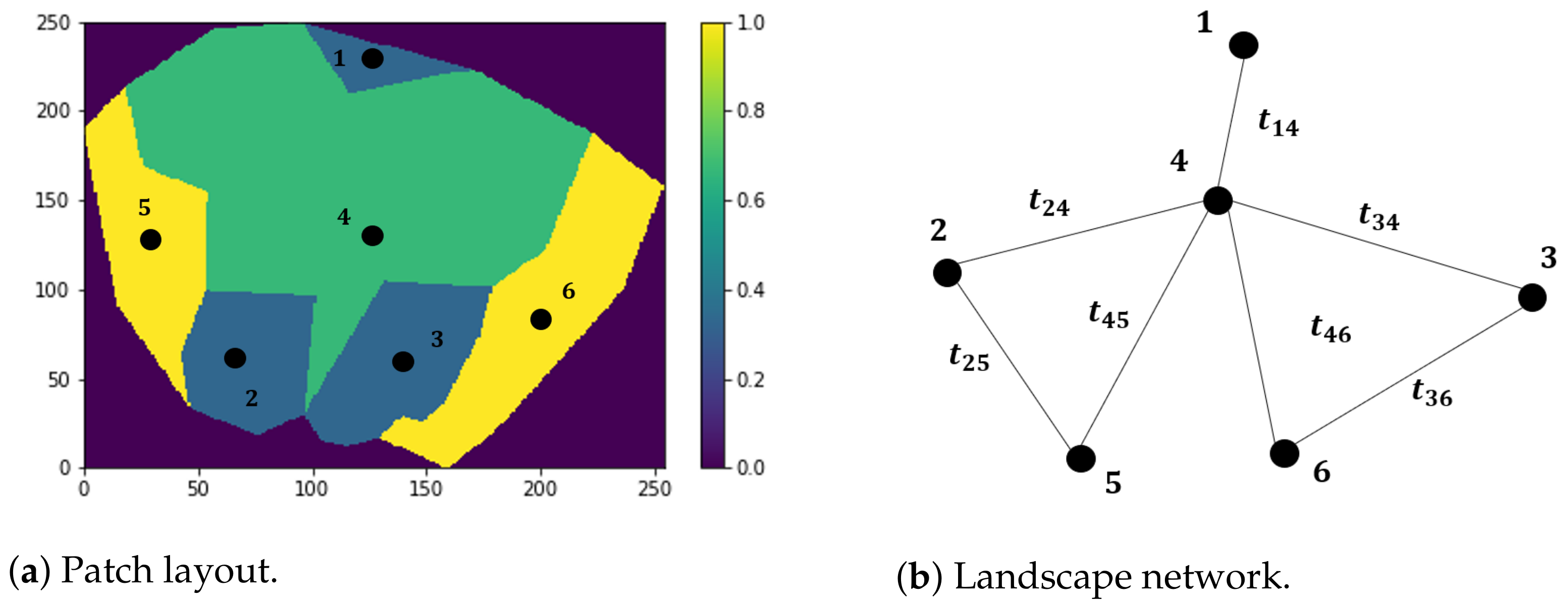
, we parametrize the landscape network, which is a graph representation of the layout of the land patches, as we can see in
Figure 1.
The shape of the border of each patch is only taken into account in cellular automaton simulations. Instead of attributing mean probability values to each edge of the landscape network, we consider instead the transition probabilities in each pair of cells . The resulting time values are affected by these probabilities. In addition, if a connection between two nodes is not suitable for fire spread, local transition probabilities will inhibit the process and the fire will never reach the respective neighbour. Thus, the network’s parametrization should account probability information which, in turn, depends on the accuracy of the study of the terrain.
Mathematically, our landscape network can be expressed as
This network is directional, but the direction of the edges is determined by the ignition point and the edge values, determined by local dynamics. Determining the path of the fire throughout the edges will always depend on the specific real-case application of the dynamics of each patch and their respective layout.
The ArcMap generated layout image comprises
polygons. Each polygon represents a land patch and can take one of the three possible class values. A class value is a generic attribute that we associated to each patch to characterize them. In a real-case scenario, this class value is substituted by a value that depends on FWT conditions, and affects the transition probability of each cell in the correspondent polygon. The adjacency matrix of this landscape network can be written as
and the time-weighted adjacency matrix is given by
In general, , but because the patch layout is fixed, G is symmetric, while is not symmetric in its values. For a certain pair of nodes , the path is different than the path , due to different patch characteristics and the randomness in the respective trajectories. The equivalence in a spread of a disease is the latency period, i.e., the time interval between the infection of an individual and the instant from when the individual becomes capable of infecting others. In this equivalence, each patch corresponds to an individual, the instant of infection is the instant of the first ignition and the instant when the individual infects others is the instant when the fire reaches other patches. Thus, we can consider the latency period as the time the fire travels from the first ignition at node p to its neighbour q.
The importance of representing a fire spreading dynamics on a network of networks is that each node may be treated individually, according to its own characteristics, but independently of the rest of the nodes. The knowledge of the spreading time is useful for the articulation of the protection forces when it comes to fighting the advancing fire.
One of the most common network measures that can contribute to this articulation is the geodesic distance, i.e., the shortest network distance between a pair of nodes, or the smallest value of
r such that
. In our case, we use propagation time, which is deeply related to distance. Thus, our
mean geodesic time from
p to
q, averaged over all nodes
q in the network is given as
where
is the time duration for fire spread from node
p to node
q and
n is the number of nodes of the landscape network. The average over all
of Equation (
10) is the mean time spent between all pairs of nodes, the average landscape spreading time,
The fire-break structure should act in a way as to interfere with the most likely and the quickest path of propagation of the fire.
Let us consider a region with a central response command (CRC), whose function is to detect, monitor and fight against forest fires in that region, using every means possible for the effect. Let us assume that the expected response time, , is defined as the time spent from the instant of the initial ignition until the instant that the any direct action against fire starts. We assume here that, at the moment of the ignition, the CRC is immediately aware of the fire occurrence and we do not consider any variable during the process of mobilization of CRC. For that specific region, we must verify , at least for the paths with the highest probabilities of fire spread. In the graph of that region, for instance, we need to sequentially cut the paths with the smallest . A fire-break structure must be implemented in order to satisfy this condition.
Other centrality measures are computed as well, such as degree, betweenness, closeness and eigenvector centralities,
where, in Equation (
12),
are the
entries of the adjacency matrix
G; in Equation (
13),
is the number of geodesic paths connecting nodes
i and
j and
is the number of
that pass through node
p; in Equation (
14),
is the shortest distance between nodes
p and
q; in Equation (
15),
is the largest eigenvector of
G.
3. Materials
We used ArcMap from ArcGIS Desktop, version 10.8.1.14362, to build the vector and raster files used in our study. Vector file images were converted to raster type in ArcMap and the correspondent vector data was stored in .csv files, under Microsoft Excel. The created files were then used as input in the python 3.8.
The ArcMap generated raster image—our prototype image—comprises a set of class values with a certain patch layout (
Figure 1a) and was converted in python 3.8 to a
matrix, with a direct correspondence between each entry (cell) and the image pixels.
Cellular automaton simulations were run in the terrain matrix, which results from the convolution of the ArcMap converted matrix with a random matrix, meaning that the transition probabilities were calculated using the class values associated to each patch and a random component. The initial ignitions took place at each patch, in a convenient set of coordinates, .
Computation of network measures, as well as graphs and plots not related to cellular automaton simulations, were carried out in Mathematica 12.2, generously offered by SYMCOMP 2021, the 5th International Conference on Numerical and Symbolic Computation: Developments and Applications, on 25–26 March, Évora, Portugal, under the Young Research Awards.
4. Results
We worked over an
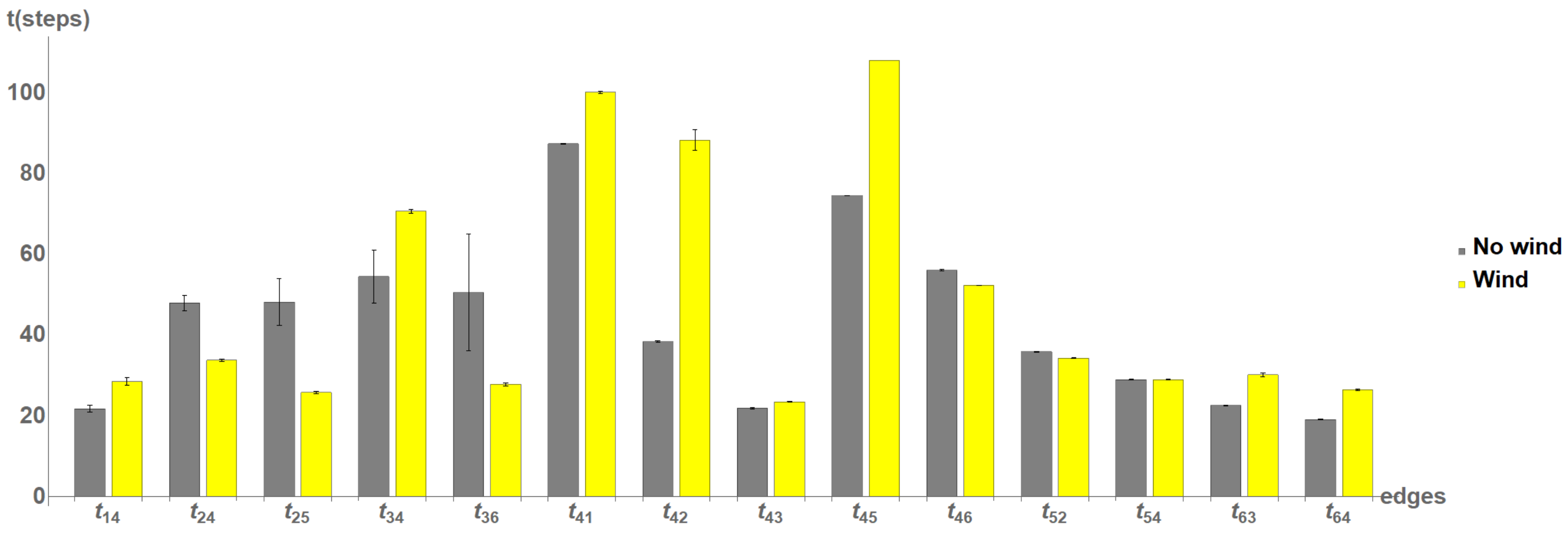
ArcMap generated raster image, whose patches are drawn polygons in the associated vector file (
Figure 2a). The patch layout was intentionally aiming for simplicity to ease computational simulations. Each patch has an irregular border and is represented by a numbered node. Different colours represent patches with different types of initial FWT conditions, mentioned in
Section 1, which are translated by a
class value, represented in the colour bar. As a prototype image, it can be applied to any geography, as long as the patches are rearranged according to the respective FWT conditions (e.g., layout of different vegetation types). This can be achieved by visual recognition through satellite monitoring data.
As said in
Section 3, the input image was converted into a
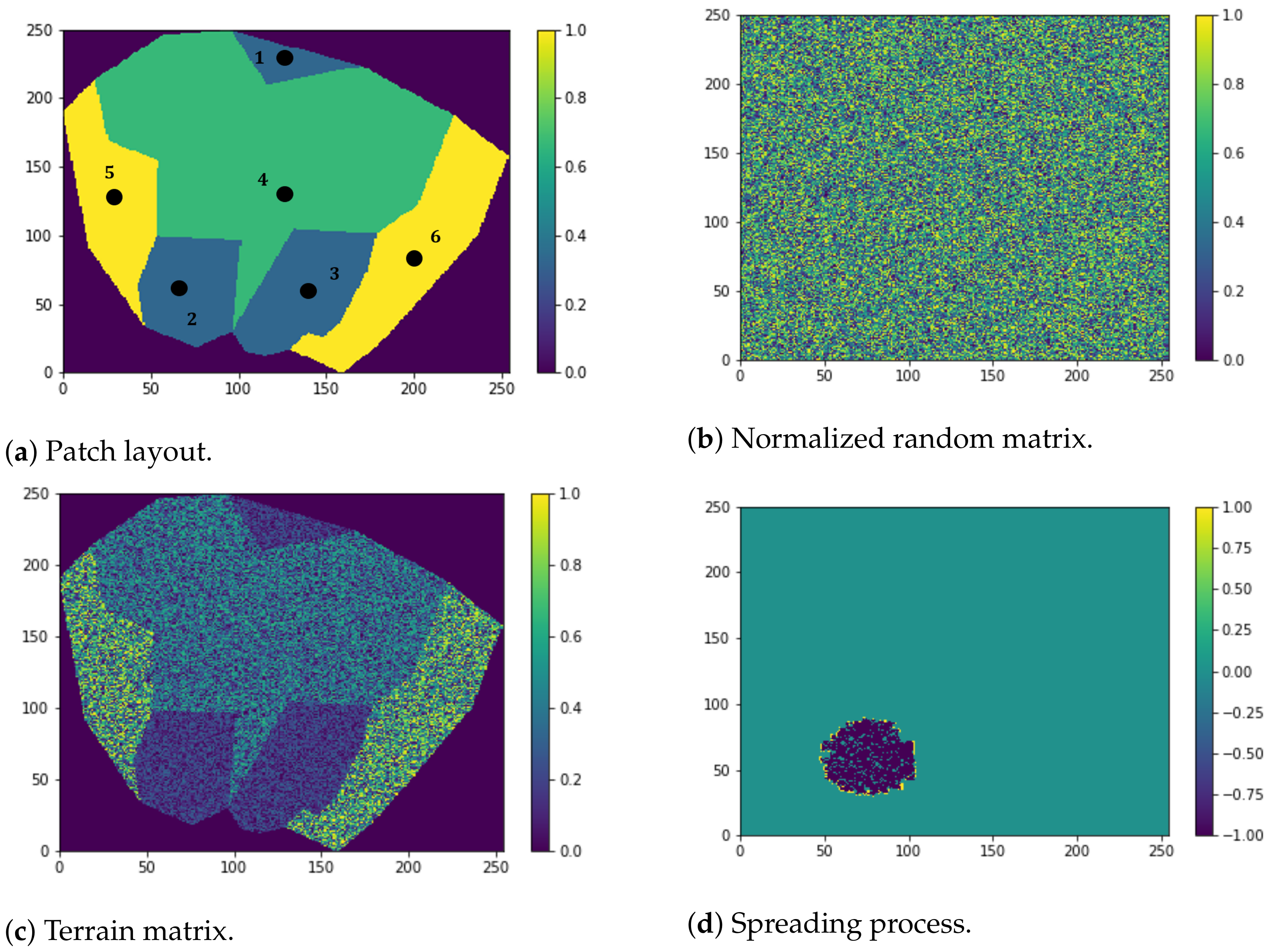
matrix. The matrix that reproduces the terrain more faithfully, in
Figure 2c, results from the convolution of matrices in
Figure 2a,b. The respective transition probabilities were used at every step of each spreading process to obtain
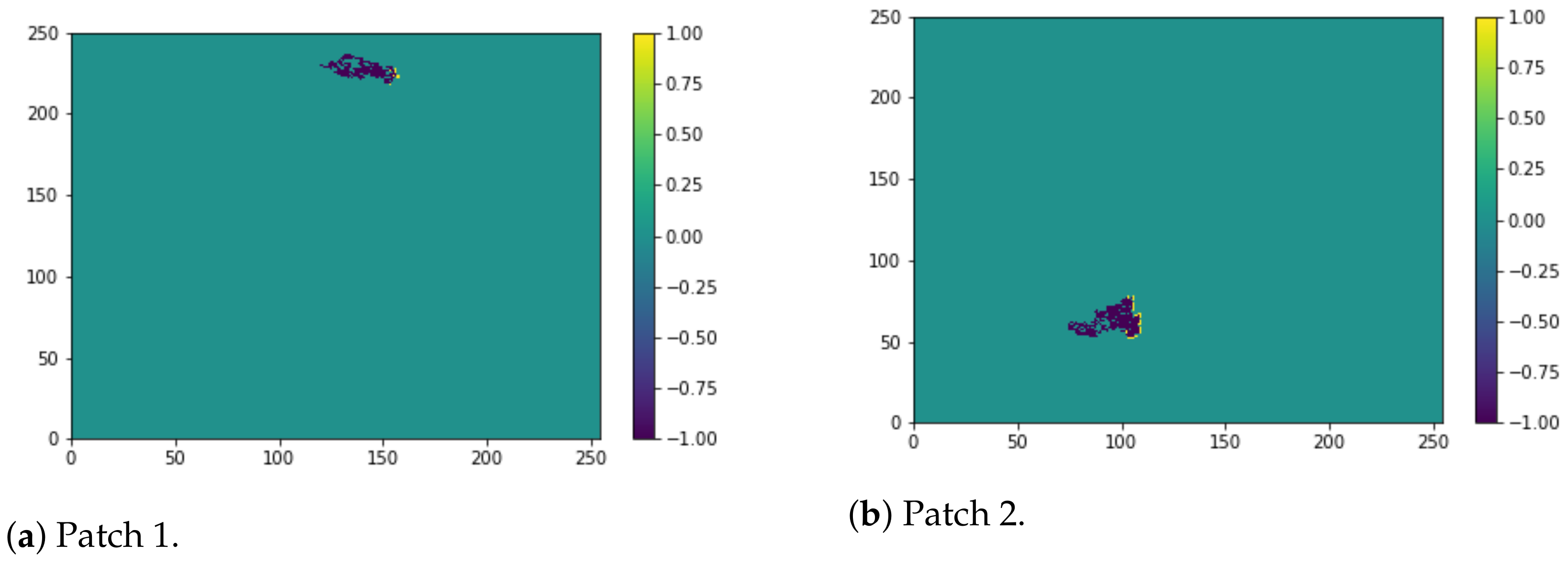
Figure 2d. The coordinates of each ignition point at each respective polygon are 1: (230, 120); 2: (60, 75); 3: (60, 140); 4: (125, 127); 5: (130, 25); 6: (90, 200).
4.1. Homogeneous Grid
For the homogeneous case in no-wind conditions, the convolution matrix attributes to each cell transition probabilities , where is the class value of polygon p, which translates its average rate of spread , and is a random number in that attributes randomness to the patch. The calculus of the value should include the parameters as the representative measures of FWT conditions, but in this prototype image, for simplicity, we use a random number.
The rules for fire contamination apply under the general condition , where is a random number generated at every step of the process and is a fixed value established previously, also between 0 and 1. We ran 100 simulations for values of from to in increments of and calculated the average time duration of the spreading process for each polygon. The break condition was the instant at which an infected cell no longer belonged to the patch at which the process took place.
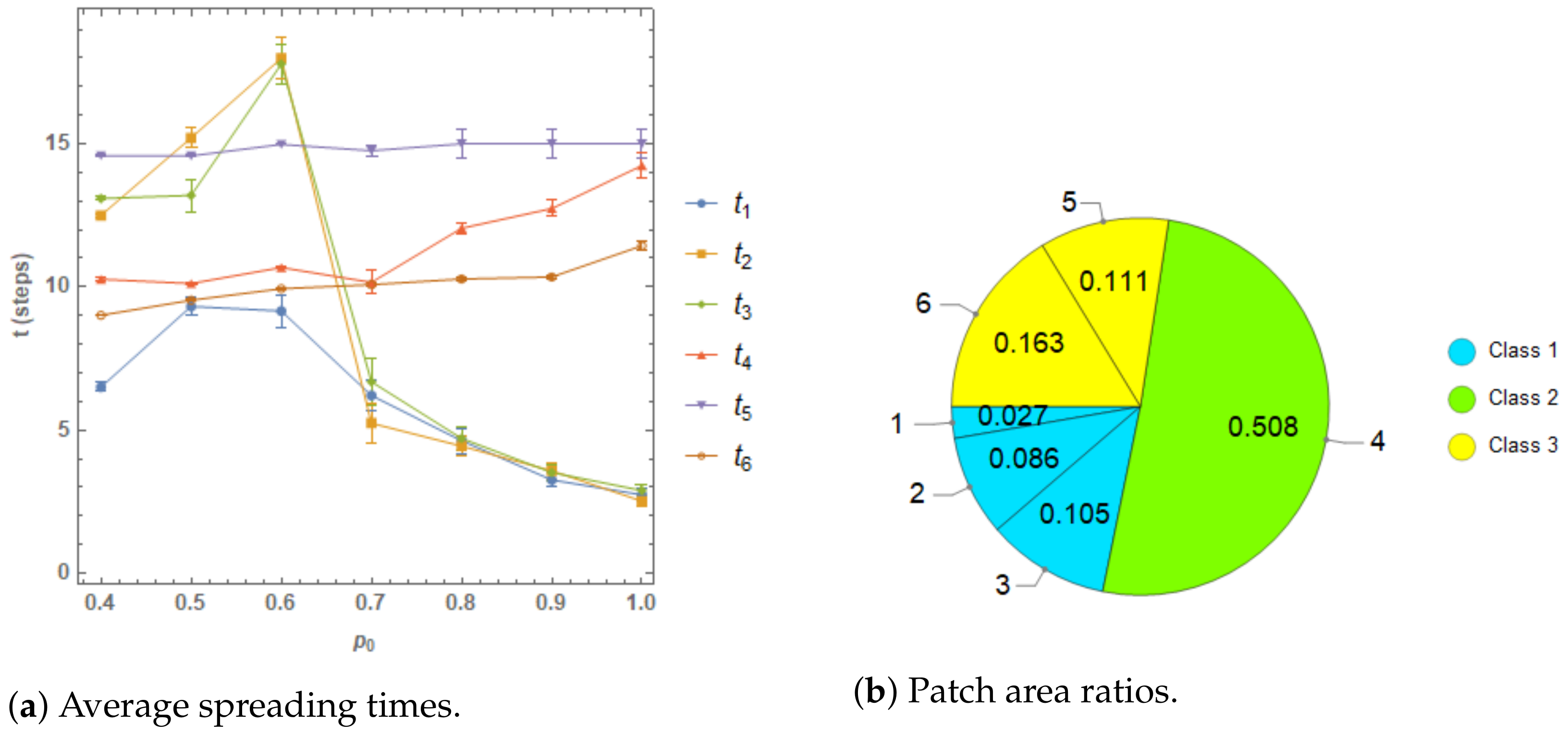
Figure 3a shows the time averages of the spreading process for each patch as function of
. Spreading time for patches 1, 2 and 3, with
,
, decreases with
and converges to approximately 3 time steps, most probably from the lack of burning cells for the next infection. We also observe an “inflection point” at
. The initial increase, from
to
is present in those three spreading simulations, but with lower values for
, which might be related to the fact that patch 1 has the smaller area among all the patches, as shown in
Figure 3b. Patch
, with
is approximately constant along
values. Patch
, with
, shows a slight increase with
, alongside with
, of
—the latter with the largest area.
Figure 3b shows the area of each patch in proportion to the sum of the area of all patches.
4.2. Heterogeneous Grid
The heterogeneous case is analogous to the homogeneous one, but we now consider different patches and, therefore, different values, translated by different . Each cell has, again, randomness associated . With different patches to consider, we now consider both ways of spreading between each pair of nodes, that is, , since the path taken by the fire is always in respect to the origin patch, with the original FWT conditions.
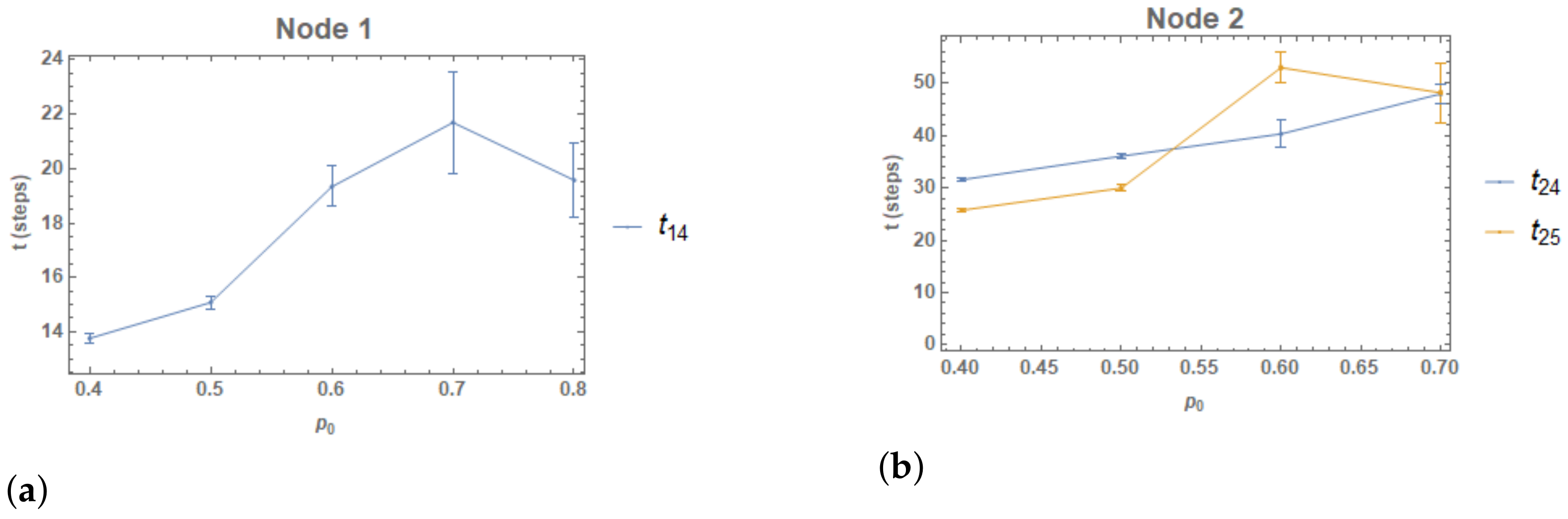
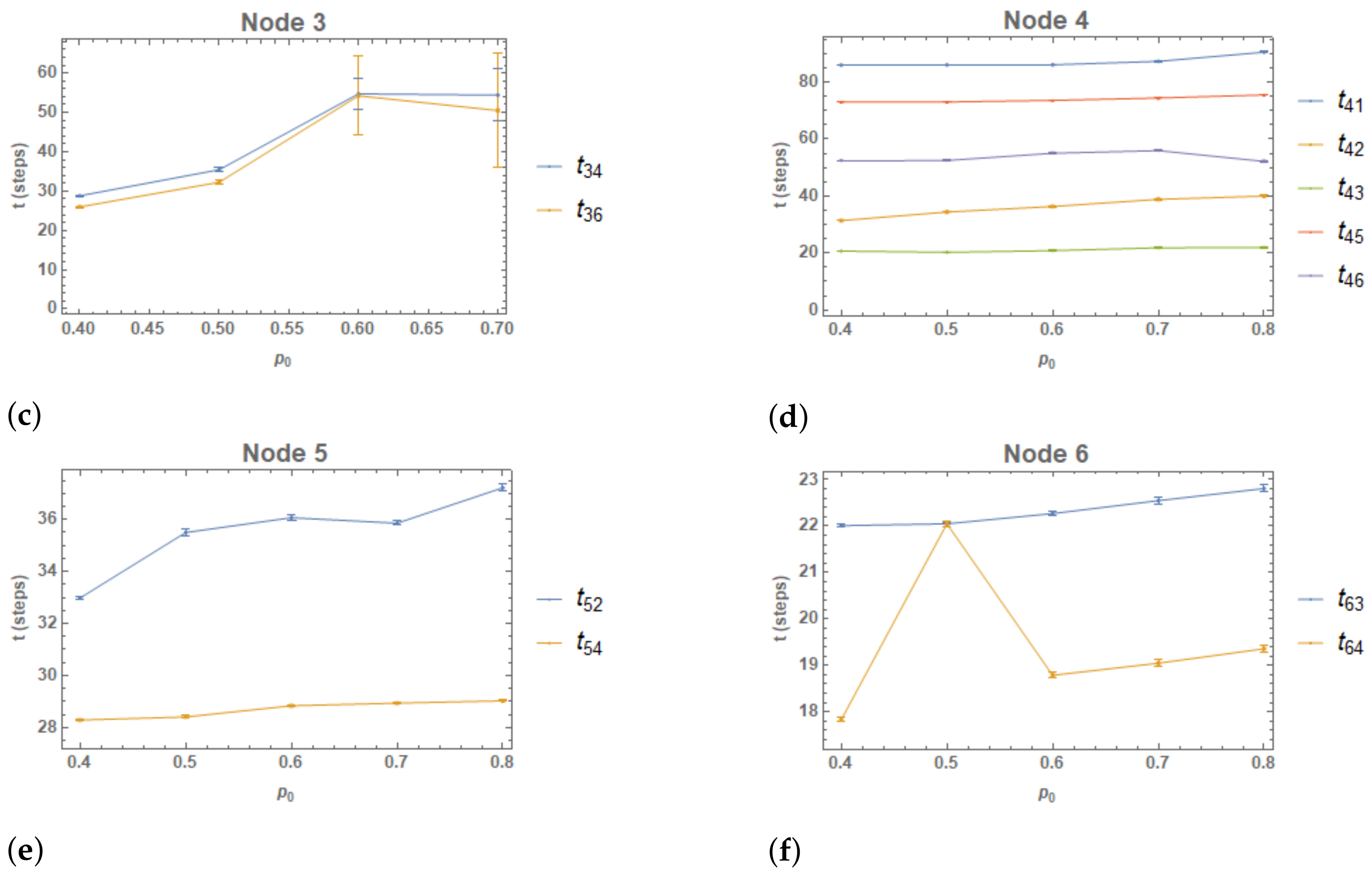
Figure 4 shows the evolution of the averaged spreading time for each node patch and for each directed edge, in number of steps. In general, average spreading time durations increase with
. Node 1 shows an irregular increase and also an increase in the standard deviation error. The edges of node 2 have approximately the same average slope. They differ in behaviour at
, and the error also increases with
. In node 3, the edges have a similar behaviour, but with an error that compromises the increasing pattern. The edges
have the lowest increase rate and the values
are approximately regularly spaced. Edges
and
differ in slope and behaviour throughout the range of
values. Edges
and
also differ in their behaviour, although from
onwards, the slope and constancy is similar, with different values of spreading time.
4.3. Influence of a Vectorial Component
Under the effect of a vectorial component, our condition to perform the simulations was , where represents the vectorial influence on the spreading process, with , ; works as a measure of the intensity of that influence; the random number introduces randomness into the whole process.
Cellular automaton simulations in
Figure 5 show the wind effect towards East, with
, for each patch of our prototype image. That effect is also represented in
Figure 6.
As the fire front is represented in yellow in
Figure 5, we see a right leaning tendency for the distribution of burning cells. For situations in
Figure 5c,d,f, we observe a well defined vertical line, in yellow, perpendicular to
, suggesting the saturation of the fire front in that direction. Each subfigure corresponds to a time step in one of 100 simulations for the respective node patch. Due to the randomness introduced, all of the outcomes referring to cell layout are different, so these images are merely illustrative of the spreading process simulations.
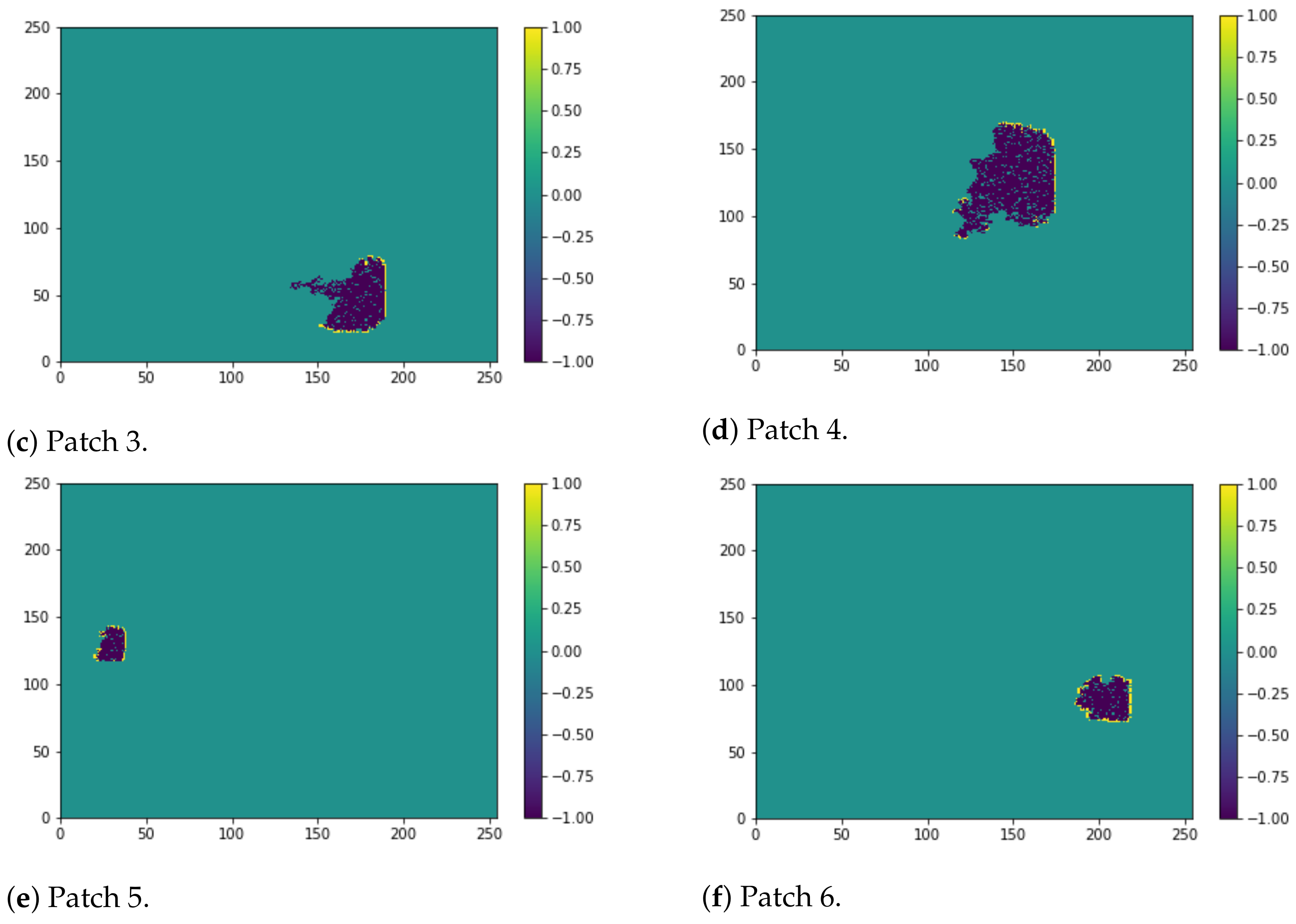
In the bar chart of
Figure 6, we can compare the average spreading time results for the no-wind and wind cases, which is also reflected in the relative increase in spreading time, in
Figure 7f.
4.4. Landscape Network
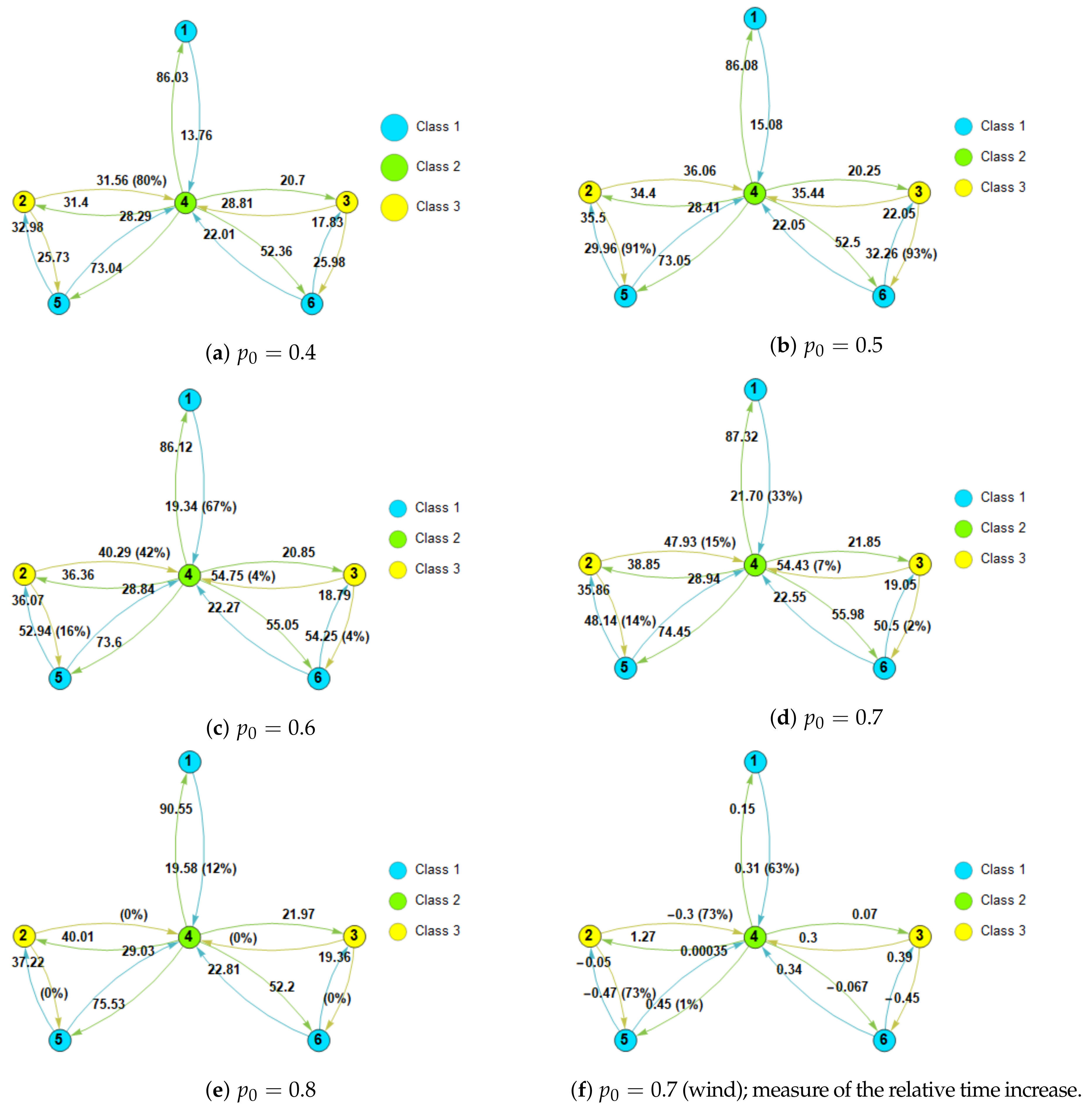
Based on the spreading time results from local dynamics, we build a representative network of the patch layout for different values of
, as shown in
Figure 7. The landscape networks are parametrized by the average spreading time values, as a result of given FWT conditions, which were translated by the parameter
in cellular automaton simulations. We also computed some overall network measures, such as the mean distance, edge connectivity, diameter and assortativity, listed in
Table 1, and the mentioned centrality measures, shown in
Figure 8.
By analysing
Table 1, we see that the mean distance, edge connectivity and diameter tend to increase, although for
these values are either null or invalid. This is because the success rate in the spreading process was null (shown in
Figure 7e as a null percentage,
) and, therefore, those connections were cut off. Negative values for assortativity naturally show a correlation between nodes of different degree, which is a direct consequence of the way the patches were drawn (ideally based on map observance and FWT conditions). The results for the presence of wind are the highest among all the results for these measures.
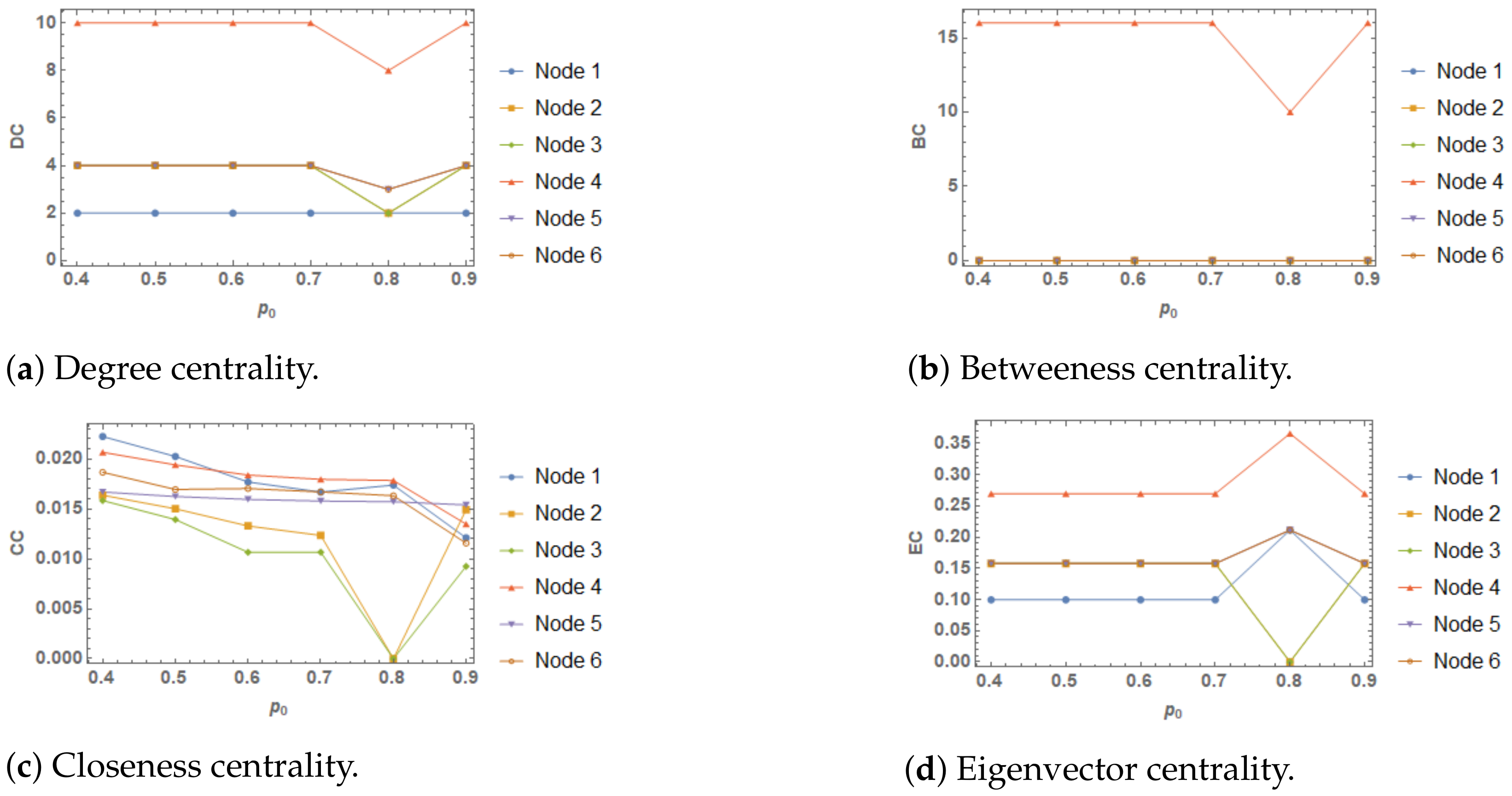
We computed the centrality measures (Equations (
12)–(
15)) using
Wolfram Mathematica software. The results for the nodes {1, 2, 3, 4, 5, 6} are shown in
Figure 8.
By analysing
Figure 8, the degree centrality shows the number of edges for each node, which only varies for the case where
, based on the null success rate of fire spread throughout the patch for nodes 2 and 3. This reflects on edges
,
,
and
being cut off.
While betweenness centrality is only non-null for node 4, closeness centrality shows a decreasing pattern with , with a null value for nodes 2 and 3, in the situation . Eigenvector centrality is constant with , but varies for every node in when .
5. Discussion
Results for the heterogeneous grid, where we only analyse the spreading process in a node patch, reveal the same decreasing tendency for patches 1, 2, 3, with
, for increasing values of
. Given the discrepancy of terrain values and
at each step, infection becomes more difficult, which leads to the break of the spreading process after approximately 3 time steps, as shown in
Figure 3a. Primarily, one should aim for such terrain conditions in order to achieve fire spread mitigation. Nodes 4, 5 and 6 don’t reveal a decreasing tendency, so there is a higher risk of infecting neighbours in comparison to other nodes, although in this analysis we lack the correlation with the area of each patch.
In the heterogeneous grid, for each node we associate a similar behaviour between edges, provided the class of the node, , is the same. The difference in average spreading time values is due to the distance from the ignition point to the next neighbour. A similar behaviour is observed in nodes 2, 3, 4 and 6, although the latter presents the edge , with an atypical spreading time point value for .
Cellular automaton simulations were visually monitored through images such as those presented in
Figure 2d and
Figure 5, which were generated every simulation, at every time step. This helped us control simulation results in terms of expected fire spread behaviour, based on the literature. For example, following [
10], typically, wildfires begin from a single source and spread outward, growing in size and assuming an elliptical shape with the major axis in the direction most favourable to spread, which we always observed for the homogeneous case, which is visually presented in
Figure 5. The presence of a vectorial component, such as wind or slope, clearly affects the average spreading time. In
Figure 7f we observe, for the left-right oriented edges, either a negative or a small value in terms of the relative increase when faced to
Figure 7d (
,
),
,
,
,
), while for the right-left oriented edges, a general increase in the same values (
,
,
,
,
,
). Values
and
don’t coincide with the tendency, with a success rate of
.
The landscape network is built based on average spreading time values. These values vary with the parameter , which could reflect, for instance, the variation in the vegetation over the seasons, and the presence of a vectorial component, such as wind or slope. The rate of success in fire spread, expressed as a percentage along the edges, varies according to each case. The implementation of a fire-break should act in such a way as to mitigate fire spread throughout the edges with lower values of and higher probability, especially in nodes with high centrality values. That depends on previous knowledge on FWT conditions. With this test case, with a random scenario for such conditions, we intend to expose the structure of our model, leaving the establishment of an adequate fire-break structure in a real-case scenario for further work.
This work shows a network model for predicting fire spread in specific terrain, fuel and weather conditions. Our multi-scale approach allows real-time simulations, which can be an added value for measures adopted by the civil protection forces and other competent authorities when fighting forest fires. Additionally, our model doesn’t specify a method for terrain characterization (satellite image recognition, land probing, terrain survey, etc.), therefore area and rate of spread, whether at the cell or at the patch range, are assessed by prior knowledge, usually available to authorities.
Results indicate the importance of transition probabilities from one cell to another, which we associated to fuel availability. Work has already been done with cellular automata to model fire spread [
14], although our focus is on average spreading time, in order to construct an effective landscape network. One advantage of dividing the land in patches is that it allows gathering information of smaller areas easier in comparison to larger ones, in general.
Computing the spreading time under different terrain, fuel availability and weather conditions may be an important contribution to time management in the event of a forest fire and may also help to mitigate the consequences of such phenomenon.
Although real-case applications are still in progress, it’s already possible to ensure a larger structure, given time values from local dynamics. In this context, a multilayer network structure is a possible solution for our approach of contributing for the mitigation of fire spread.
6. Further Work
In this article, we built a mathematical model and we implemented a test case. As a future work we intend to study specifically the geometry of the simulated fire front and burned area, to find the best configuration for patch layout.
In the most practical scope, we intend to apply this model to a specific geography, most preferably to a well-documented wildfire-prone region of the Globe. By simulating a real-case scenario, we can analyse more deeply the effect of and of every transition probability , as well as , when dealing with the presence of wind or slope. The formula for may depend strongly on the fire model, the associated fuel model in the respective geography, and the data gathering methods used.
Varying the coordinates of the initial ignition is also important, although its importance may be emphasized at the local scale. It’s specially important to vary the initial ignition when dealing with a real-time case simulation, with well-defined and well-known FWT conditions.
In a real-case scenario, after getting knowledge of the spreading times for a collection of connected patches, we intend to use the obtained time values to parametrize the landscape network. With the final structure of a networks of networks, we study its connectivity. The main goal is to gather cut-sets solutions (as fire-breaks) with the best relation cost-effectiveness.
The overall study will also be complemented by comparing spreading results with burned areas of previous fire events. This comparison should act as calibration factor for data refinement regarding FWT conditions. Although this comparison is possible, we also need to consider human intervention to stop the fire and its effect on the shape of the burned areas, which is a challenge to overcome. The information regarding human intervention is accessed through the civil protection forces.
Author Contributions
Conceptualization, M.C.G. and N.A.R.; methodology, S.P., M.C.G., N.A.R. and L.M.L.; software, S.P.; validation, S.P., M.C.G. and N.A.R.; formal analysis, S.P.; investigation, S.P.; resources, S.P., M.C.G. and N.A.R.; data curation, S.P.; writing—original draft preparation, S.P.; writing—review and editing, M.C.G., N.A.R. and L.M.L.; visualization, S.P.; supervision, M.C.G. and N.A.R.; project administration, M.C.G. and N.A.R.; funding acquisition, M.C.G. and N.A.R. All authors have read and agreed to the published version of the manuscript.
Funding
This research was partially sponsored with national funds through the Fundação Nacional para a Ciência e Tecnologia, Portugal-FCT, under projects UIDB/04674/2020 (CIMA) and UIDP/04683/2020 (ICT). Project CILIFO (Iberian Center for the Investigation and Fighting of Forest Fires) (0753_CILIFO_5_E), under which this study is currently being developed, is 75% financed by the Cross-border Cooperation Program Interreg VA Spain-Portugal–Interreg POCTEP (2014–2020).
Acknowledgments
The authors gratefully thank to Pedro Nogueira and João Ribeiro, from the University of Évora, to José Fernando Mendes, from University of Aveiro, to the institutions CIMA and ICT and finally to the project CILIFO.
Conflicts of Interest
The authors declare no conflict of interests.
References
- Nunes, L.J.R.; Meireles, C.I.R.; Pinto Gomes, C.J.; Almeida Ribeiro, N.M.C. Socioeconomic aspects of the forests in Portugal: Recent evolution and perspectives of sustainability of the resource. Forests 2019, 10, 361. [Google Scholar] [CrossRef] [Green Version]
- Young, J.A.; Evans, R.A. Population dynamics after wildfires in sagebrush grasslands. Rangel. Ecol. Manag. J. Range Manag. Arch. 1978, 31, 283–289. [Google Scholar] [CrossRef] [Green Version]
- Maselli, F.; Rodolfi, A.; Bottai, L.; Romanelli, S.; Conese, C. Classification of Mediterranean vegetation by TM and ancillary data for the evaluation of fire risk. Int. J. Remote Sens. 2000, 21, 3303–3313. [Google Scholar] [CrossRef]
- Fernández, C.; Vega, J.A.; Fonturbel, T.; Pérez-Gorostiaga, P.; Jiménez, E.; Madrigal, J. Effects of wildfire, salvage logging and slash treatments on soil degradation. Land Degrad. Dev. 2007, 18, 591–607. [Google Scholar] [CrossRef]
- Heymes, F.; Aprin, L.; Ayral, P.A.; Slangen, P.; Dusserre, G. Impact of wildfires on LPG tanks. Chem. Eng. Trans. 2013, 31, 637–642. [Google Scholar]
- Fons, W.L. Analysis of fire spread in light forest fuels. J. Agric. Res. 1946, 72, 93–121. [Google Scholar]
- Riaño, D.; Chuvieco, E.; Salas, J.; Palacios-Orueta, A.; Bastarrika, A. Generation of fuel type maps from Landsat TM images and ancillary data in Mediterranean ecosystems. Can. J. For. Res. 2002, 32, 1301–1315. [Google Scholar] [CrossRef]
- Menezes, I.C.; Freitas, S.R.; Lima, R.S.; Fonseca, R.M.; Oliveira, V.; Braz, R.; Dias, S.; Surový, P.; Ribeiro, N.A. Application of the Coupled BRAMS-SFIRE Atmospheric and Fire Interactions Models to the South of Portugal. Rev. Bras. Meteorol. 2021. [Google Scholar] [CrossRef]
- Ivanilova, T.N. Set probability identification in forest fire simulation. Annu. Rev. Autom. Program. 1985, 12, 185–188. [Google Scholar] [CrossRef]
- Rothermel, R.C. A Mathematical Model for Predicting Fire Spread in Wildland Fuels; US Department of Agriculture, Forest Service, Intermountain Forest & Range Experiment Station: Ogden, UT, USA, 1972; Volume 115.
- Anderson, H.E. Aids to Determining Fuel Models for Estimating Fire Behavior; US Department of Agriculture, Forest Service, Intermountain Forest and Range Experiment Station: Ogden, UT, USA, 1981; Volume 122.
- Scott, J.H. Standard Fire Behavior Fuel Models: A Comprehensive Set for Use with Rothermel’s Surface Fire Spread Model; US Department of Agriculture, Forest Service, Rocky Mountain Research Station: Fort Collins, CO, USA, 2005.
- O’Connor, T.G.; Uys, R.G.; Mills, A.J. Ecological effects of fire-breaks in the montane grasslands of the southern Drakensberg, South Africa. Afr. J. Range Forage Sci. 2004, 21, 1–9. [Google Scholar] [CrossRef]
- Russo, L.; Russo, P.; Evaggelidis, I.N.; Siettos, C. Complex network statistics to the design of fire breaks for the control of fire spreading. Chem. Eng. Trans. 2015, 43, 2353–2358. [Google Scholar]
- Buscarino, A.; Famoso, C.; Fortuna, L.; Frasca, M.; Xibilia, M.G. Complexity in forest fires: From simple experiments to nonlinear networked models. Commun. Nonlinear Sci. Numer. Simul. 2015, 22, 660–675. [Google Scholar] [CrossRef]
- Russo, L.; Russo, P.; Siettos, C.I. A complex network theory approach for the spatial distribution of fire breaks in heterogeneous forest landscapes for the control of wildland fires. PLoS ONE 2016, 11, e0163226. [Google Scholar] [CrossRef] [PubMed]
- Karafyllidis, I.; Thanailakis, A. A model for predicting forest fire spreading using cellular automata. Ecol. Model. 1997, 99, 87–97. [Google Scholar] [CrossRef]
- Grácio, M.C.; Fernandes, S.; Lopes, L.M. Full-commanding a network: The dictator. In Proceedings of the International Conference on Complex Networks and Their Applications, Cambridge, UK, 11–13 December 2018; pp. 505–511. [Google Scholar]
- De Domenico, M.; Granell, C.; Porter, M.A.; Arenas, A. The physics of spreading processes in multilayer networks. Nat. Phys. 2016, 12, 901–906. [Google Scholar] [CrossRef] [Green Version]
- Boccaletti, S.; Bianconi, G.; Criado, R.; Del Genio, C.I.; Gómez-Gardenes, J.; Romance, M.; Sendina-Nadal, I.; Wang, Z.; Zanin, M. The structure and dynamics of multilayer networks. Phys. Rep. 2014, 544, 1–122. [Google Scholar] [CrossRef] [PubMed] [Green Version]
- Kivelä, M.; Arenas, A.; Barthelemy, M.; Gleeson, J.P.; Moreno, Y.; Porter, M.A. Multilayer networks. J. Complex Netw. 2014, 2, 203–271. [Google Scholar] [CrossRef] [Green Version]
- Aleta, A.; Moreno, Y. Multilayer networks in a nutshell. Annu. Rev. Condens. Matter Phys. 2019, 10, 45–62. [Google Scholar] [CrossRef] [Green Version]
- Newman, M.E.J. The structure and function of complex networks. SIAM Rev. 2003, 45, 167–256. [Google Scholar] [CrossRef] [Green Version]
Figure 1.
(a) Layout of some irregular-shaped patches, numbered from 1 to 6. Different colours represent different class values, from 0 to 1 (vector image generated in ArcMap and converted into raster format); (b) graph representation of the patch layout, as the landscape network parametrized by time values tij distributed along the edges (i, j).
Figure 2.
(a) is an ArcMap generated image, where the polygons were manually drawn into a vector file, which was converted to a raster format thereafter, and then converted into a matrix; (b) is a python-generated matrix, with random entries between 0 and 1; (c) results from the convolution between matrices (a,b); and (d) is an example of a spreading process occurring in polygon 5 of the terrain matrix (c), with starting ignition at coordinates (60, 75). The state correspondence of the ith cell is unburned: si = 0, burning: si = 1, burned: si = −1.
Figure 3.
(a): average spreading time duration for patches {1, 2, 3, 4, 5, 6}. Each time unit represents a computational step. The horizontal axis represents an increase in p0 values. Each point series corresponds to the average spreading time over 100 simulations within a patch, starting from the each ignition point. The break condition for the spreading process was the time step at which an infected cell reached a neighbouring patch or the lack of burning nodes for infection in the next step. (b): representation of patch areas, in relation to the total layout.
Figure 4.
Average spreading time results for each patch. Each time series is in respect to each directed edge. Each point corresponds to a time value, averaged over 100 simulations within the patch it refers to.
Figure 4.
Average spreading time results for each patch. Each time series is in respect to each directed edge. Each point corresponds to a time value, averaged over 100 simulations within the patch it refers to.
Figure 5.
Spreading results in the cellular automaton , for and wind oriented towards East, with the vectorial component . In green, the unburned cells (), in yellow, the fire front () and in blue, the burned cells (). Each image corresponds to a specific time step in the sequence of 100 simulations.
Figure 6.
Average spreading time values for each of the edges . In gray, no wind situation; in yellow, the same simulations performed with the action of the wind. Simulations were performed for .
Figure 6.
Average spreading time values for each of the edges . In gray, no wind situation; in yellow, the same simulations performed with the action of the wind. Simulations were performed for .
Figure 7.
Graph schemes of the patch layout for different values of p0. Edge values correspond to averaged spreading time values. Graph from (f) is parametrized with the measure of time increase in relation to (d).
Figure 7.
Graph schemes of the patch layout for different values of p0. Edge values correspond to averaged spreading time values. Graph from (f) is parametrized with the measure of time increase in relation to (d).
Figure 8.
Centrality measures of the the landscape network for different nodes and different values of p0.
Figure 8.
Centrality measures of the the landscape network for different nodes and different values of p0.
Table 1.
Network measures.
Table 1.
Network measures.
| Graph Measures∖ | 0.4 | 0.5 | 0.6 | 0.7 | 0.8 | 0.7 (Wind) |
|---|
| Mean distance (time) | 55.175 | 59.9817 | 66.8983 | 68.9357 | - | 80.5607 |
| Edge connectivity | 13.76 | 15.08 | 19.34 | 21.7 | 0.0 | 28.43 |
| Diameter | 117.59 | 122.14 | 140.87 | 141.75 | - | 162.17 |
| Assortativity | | | | | | −0.704399 |
| Publisher’s Note: MDPI stays neutral with regard to jurisdictional claims in published maps and institutional affiliations. |
© 2021 by the authors. Licensee MDPI, Basel, Switzerland. This article is an open access article distributed under the terms and conditions of the Creative Commons Attribution (CC BY) license (https://creativecommons.org/licenses/by/4.0/).


