
On a Special Weighted Version of the Odd Weibull-Generated Class of Distributions


Abstract
:1. Introduction
1.1. Background
1.2. Motivations and Contributions
- (i)
- As a basic remark, in relation to , and , the analytical complexity of is quite acceptable, with the weight function remaining simple.
- (ii)
- Let us now underline the mathematical connections behind the functions , , , and . By virtue of the result in [21], the following logarithmic holds: for , which implies that . On the other side, for any , we have , which is equivalent to ; so,Therefore, the following chain of inequalities holds: , implying the following first stochastic dominance result:In this sense, the proposed WOW-G class can be seen as an alternative to the Weibull-X, Weibull-G, and MOW-G classes. This information is important enough to warrant an investigation of the WOW-G class.
- (iii)
- In relation to the literature on distribution theory, we notice that can be expressed aswith and . Therefore, the WOW-G class appears to be a subclass of the extended odd-G class championed by [22].
- (iv)
- Last but not least, the inverse function of is quite manageable; after some operations, we findwhere denotes the quantile function (qf) of the reference distribution. This implies that the qf of the WOW-G class has an analytical expression, which will be provided later.
1.3. Structure of the Paper
2. The WOW-G Class
2.1. Presentation
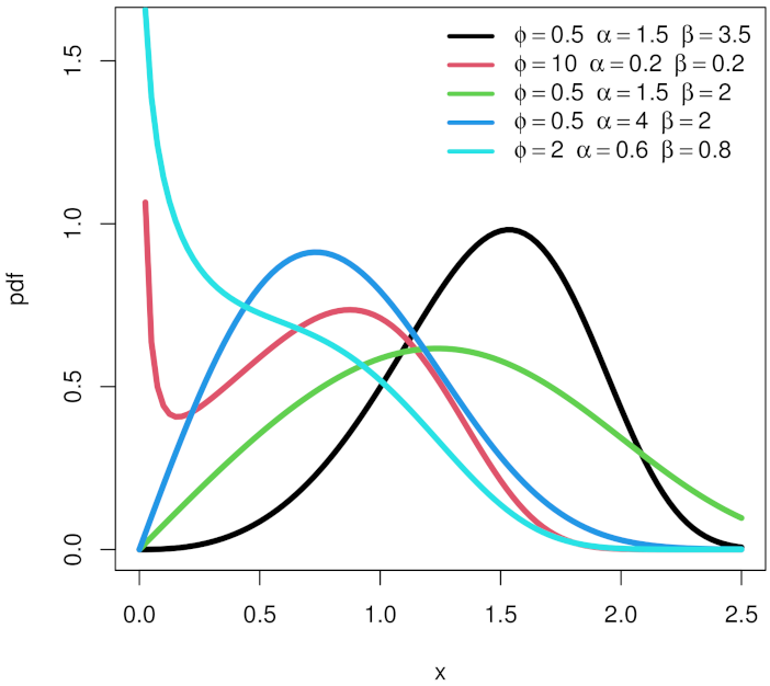
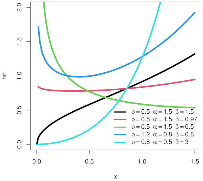
2.2. Some Examples
2.3. The WOWE Distribution
3. Theoretical Aspects
3.1. First-Order Stochastic Dominance
- For , we have ; the WOW-G class with parameter FOS dominates the WOW-G class with the parameter .
- There is no FOS property for the WOW-G class according to β.
- For any , and , we haveimplying the first result.
- For any , and , we haveThe sign of this function depends on the sign of the logarithmic term. The function is negative for x such that and positive for x such that ; the function is nonmonotonic with respect to for varying x; the FOS dominance property does not hold.
3.2. Quantile Function
3.3. Asymptotic and Form Analysis
3.4. Mixture Representation
3.5. Moments
4. Inferential Aspect
4.1. Parameter Estimation
4.2. Simulation
5. Data Analysis
5.1. Method
- (i)
- Akaike information criterion (AIC);
- (ii)
- Bayesian information criterion (BIC);
- (iii)
- consistent AIC (CAIC);
- (iv)
- Hannan–Quinn information criterion (HQIC);
- (v)
- Cramér-von Mises (W) statistic;
- (vi)
- Anderson–Darling (A) statistic;
- (vii)
- Kolmogorov–Smirnov (KS);
- (viii)
- p-value of the KS test.
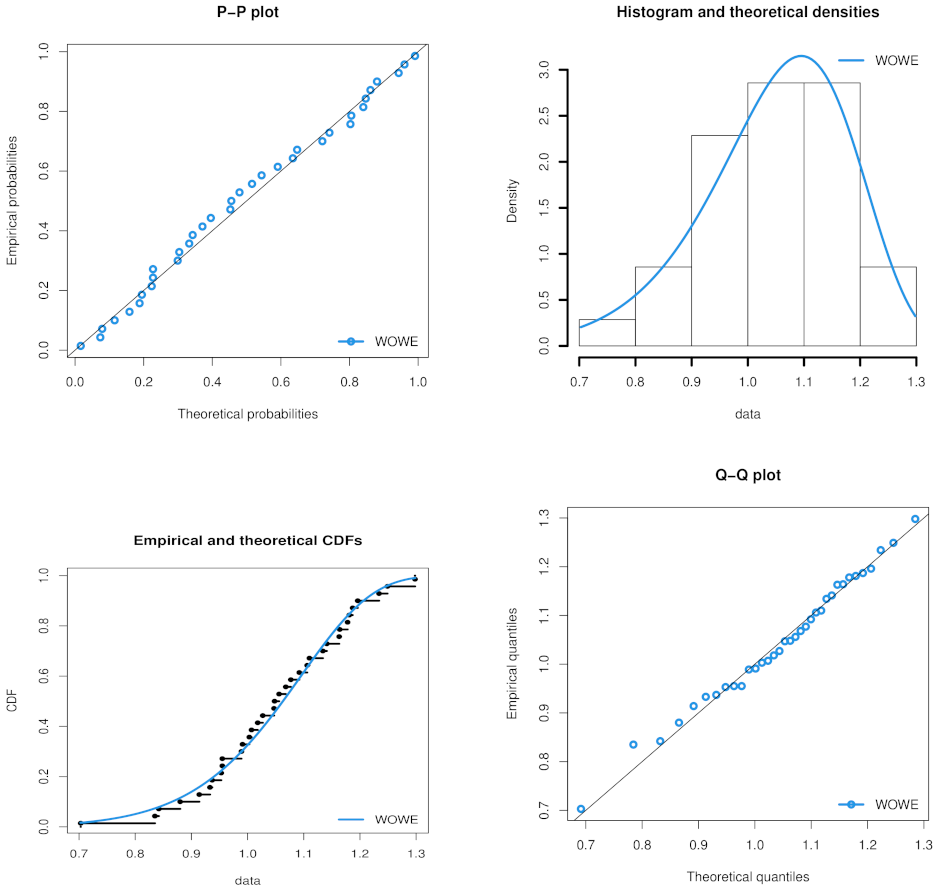
5.2. Fit of the Drilling Machine Data
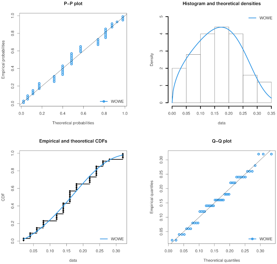
5.3. Fit of the Daily Precipitation Data
6. Conclusions
Author Contributions
Funding
Institutional Review Board Statement
Informed Consent Statement
Data Availability Statement
Acknowledgments
Conflicts of Interest
References
- Tahir, M.H.; Cordeiro, G.M. Compounding of distributions: A survey and new generalized classes. J. Stat. Distrib. Appl. 2016, 3, 1–35. [Google Scholar] [CrossRef] [Green Version]
- Brito, C.C.R.; Rêgo, L.C.; Oliveira, W.R.; Gomes-Silva, F. Method for generating distributions and classes of probability distributions: The univariate case. Hacet. J. Math. Stat. 2019, 48, 897–930. [Google Scholar]
- Cordeiro, G.M.; Silva, R.B.; Nascimento, A.D.C. Recent Advances in Lifetime and Reliability Models; Bentham Sciences Publishers: Sharjah, United Arab Emirates, 2020. [Google Scholar]
- Alzaatreh, A.; Famoye, F.; Lee, C. A new method for generating families of continuous distributions. METRON 2013, 71, 63–79. [Google Scholar] [CrossRef] [Green Version]
- Bourguignon, M.; Silva, R.B.; Cordeiro, G.M. The Weibull-G family of probability distributions. J. Data Sci. 2014, 12, 53–68. [Google Scholar] [CrossRef]
- Chesneau, C.; El Achi, T. Modified odd Weibull family of distributions: Properties and applications. J. Indian Soc. Probab. Stat. 2020, 21, 259–286. [Google Scholar] [CrossRef] [Green Version]
- Ahmad, Z.; Elgarhy, M.; Hamedani, G.G. A new Weibull-X family of distributions: Properties, characterizations and applications. J. Stat. Distrib. Appl. 2018, 5, 5. [Google Scholar] [CrossRef] [Green Version]
- Korkmaz, M.C. A new family of the continuous distributions: The extended Weibull-G family. Commun. Ser. A1 Math. Stat. 2018, 68, 248–270. [Google Scholar] [CrossRef]
- El-Morshedy, M.; Eliwa, M.S. The odd flexible Weibull-H family of distributions: Properties and estimation with applications to complete and upper record data. Filomat 2019, 33, 2635–2652. [Google Scholar] [CrossRef]
- Tahir, M.H.; Zubair, M.; Mansoor, M.; Cordeiro, G.M.; Alizadeh, M. A new Weibull-G family of distributions. Hacettepe J. Math. Stat. 2016, 45, 629–647. [Google Scholar] [CrossRef]
- Alizadeh, M.; Rasekhi, M.; Yousof, H.M.; Hamedani, G.G. The transmuted Weibull G family of distributions. Hacettepe J. Math. Stat. 2018, 47, 1–20. [Google Scholar] [CrossRef]
- Korkmaz, M.C.; Alizadeh, M.; Yousof, H.M.; Butt, N. The Generalized Odd Weibull Generated Family of Distributions: Statistical Properties and Applications. Pak. J. Stat. Oper. Res. 2018, 14, 541–556. [Google Scholar] [CrossRef] [Green Version]
- Alizadeh, M.; Jamal, F.; Yousof, H.M.; Khanahmadi, M.; Hamedani, G.G. Flexible Weibull generated family of distributions: Characterizations, mathematical properties and applications. Bucharest Sci. Bull. Ser. A Appl. Math. Phys. 2020, 82, 145–150. [Google Scholar]
- El-Morshedy, M.; Eliwa, M.S. Bivariate odd Weibull-G family of distributions: Properties, Bayesian and non-Bayesian estimation with bootstrap confidence intervals and application. J. Taibah Univ. Sci. 2020, 14, 331–345. [Google Scholar]
- El-Morshedy, M.; Eliwa, M.S.; Tyagi, A. A discrete analogue of odd Weibull-G family of distributions: Properties, classical and Bayesian estimation with applications to count data. J. Appl. Stat. 2021. [Google Scholar] [CrossRef]
- Alzaatreh, A.; Ghosh, I. On the Weibull-X family of distributions. J. Stat. Theory Appl. 2015, 14, 169–183. [Google Scholar] [CrossRef] [Green Version]
- Smith, R.L.; Naylor, J.C. A comparison of maximum likelihood and Bayesian estimators for the three-parameter Weibull distribution. Appl. Stat. 1987, 36, 358–369. [Google Scholar] [CrossRef]
- Birnbaum, Z.W.; Saunders, S.C. Estimation for a family of life distributions with applications to fatigue. J. Appl. Probab. 1969, 6, 328–347. [Google Scholar] [CrossRef]
- Bjerkedal, T. Acquisition of resistance in guinea pigs infected with different doses of virulent tubercle bacilli. Am. J. Hyg. 1960, 72, 130–148. [Google Scholar]
- Meeker, W.Q.; Escobar, L.A. Statistical Methods for Reliability Data; Wiley: New York, NY, USA, 1998. [Google Scholar]
- Topsoe, F. Some Bounds for the Logarithmic Function. Available online: https://rgmia.org/papers/v7n2/pade.pdf (accessed on 6 August 2021).
- Bakouch, H.S.; Chesneau, C.; Khan, M.N. The extended odd family of probability distributions with practice to a submodel. Filomat 2019, 33, 3855–3867. [Google Scholar] [CrossRef]
- Aarset, M.V. How to identify bathtub hazard rate. IEEE Trans. Reliab. 1987, 36, 106–108. [Google Scholar] [CrossRef]
- Shaked, M.; Shanthikumar, J.G. Stochastic Orders and Their Applications; Academic Press: New York, NY, USA, 1994. [Google Scholar]
- Gilchrist, W. Statistical Modelling with Quantile Functions; CRC Press: Abingdon, UK, 2000. [Google Scholar]
- Casella, G.; Berger, R.L. Statistical Inference; Brooks/Cole Publishing Company: Bel Air, CA, USA, 1990. [Google Scholar]
- Marinho, P.R.D.; Silva, R.B.; Bourguignon, M.; Cordeiro, G.M.; Nadarajah, S. AdequacyModel: An R package for probability distributions and general purpose optimization. PLoS ONE 2019, 14, e0221487. [Google Scholar] [CrossRef] [Green Version]
- R Development Core Team. R: A Language and Environment for Statistical Computing; R Foundation for Statistical Computing: Vienna, Austria, 2012. [Google Scholar]
- Hami Golzar, N.; Ganji, M.; Bevrani, H. The Lomax-exponential distribution, some properties and applications. J. Stat. Res. Iran 2016, 13, 131–153. [Google Scholar] [CrossRef] [Green Version]
- Nadarajah, S.; Kotz, S. The beta exponential distribution. Reliab. Eng. Syst. Saf. 2006, 91, 689–697. [Google Scholar] [CrossRef]
- Dara, S.T.; Ahmad, M. Recent Advances in Moment Distribution and Their Hazard Rates; LAP LAMBERT Academic Publishing: Chisinau, Moldova, 2012. [Google Scholar]
- Konishi, S.; Kitagawa, G. Information Criteria and Statistical Modeling; Springer: New York, NY, USA, 2007. [Google Scholar]
- Dasgupta, R. On the distribution of Burr with applications. Sankhya 2011, 73, 1–19. [Google Scholar] [CrossRef]
- Khaleel, M.A.; Ibrahim, N.A.; Shitan, M.; Merovci, F.; Rehman, E. Beta Burr type X with application to rainfall data. Malays. J. Math. Sci. 2017, 11, 73–86. [Google Scholar]
- Bilal, M.; Mohsin, M.; Aslam, M. Weibull-exponential distribution and its application in monitoring industrial process. Math. Probl. Eng. 2021, 2021, 13. [Google Scholar] [CrossRef]
- Klakattawi, H.S. The Weibull-gamma distribution: Properties and applications. Entropy 2019, 21, 438. [Google Scholar] [CrossRef] [Green Version]


| WOW-G | Reference | Domain | Num. of Par. | ||
|---|---|---|---|---|---|
| WOWU | Uniform | 3 | |||
| WOWTP | Topp–Leone | 3 | |||
| WOWE | Exponential | 3 | |||
| WOWIE | Inverse exp. | 3 | |||
| WOWW | Weibull | 4 | |||
| WOWLom | Lomax | 4 | |||
| WOWGu | Gumbel | 3 | |||
| WOWLog | Logistic | 3 |
| 7.7459 | 545.4638 | 42424.6700 | 3478367 | 22.0332 | 2.8681 | 9.3350 | |
| 18.12071 | 1206.8810 | 90740.4800 | 7265826 | 29.6398 | 1.4221 | 1.4814 | |
| 16.6674 | 481.3052 | 16555.54 | 630853.9 | 14.2654 | 0.6027 | 4.6662 | |
| 2.5418 | 23.3260 | 328.6222 | 5764.03 | 4.1067 | 2.6507 | 10.2090 | |
| 1.2709 | 5.8315 | 41.0777 | 360.2519 | 2.0533 | 2.6507 | 11.45969 | |
| 2.8451 | 9.2991 | 33.4134 | 128.8816 | 1.0974 | 0.0775 | 71.6438 | |
| 1.9195 | 4.0841 | 9.3549 | 22.6830 | 0.6319 | 242.1780 | ||
| 6.3961 | 42.1459 | 284.6251 | 1962.7610 | 1.1113 | 864.7704 |
| Sample Size | Actual Values | Average Estimate | Root-Mean-Square Error | ||||||
|---|---|---|---|---|---|---|---|---|---|
| 35 | 1.3 | 3.2 | 2.4 | 1.2811 | 4.4673 | 2.6784 | 5.1833 | 3.9974 | 0.8393 |
| 50 | 1.2842 | 4.1085 | 2.5299 | 4.4961 | 3.8963 | 0.7740 | |||
| 100 | 1.1629 | 3.3056 | 2.4306 | 0.6595 | 1.0978 | 0.6055 | |||
| 200 | 1.2056 | 3.2039 | 2.3994 | 0.5860 | 0.7956 | 0.5456 | |||
| 300 | 1.2439 | 3.1723 | 2.3765 | 0.5324 | 0.6722 | 0.5382 | |||
| 400 | 1.2819 | 3.1295 | 2.3384 | 0.5148 | 0.5818 | 0.5072 | |||
| 500 | 1.2917 | 3.1314 | 2.3424 | 0.4666 | 0.5356 | 0.4764 | |||
| 35 | 1.1 | 2.0 | 0.8 | 1.84938 | 2.9949 | 0.9004 | 0.8098 | 1.7134 | 0.2838 |
| 50 | 0.9228 | 2.4632 | 0.8454 | 0.7457 | 1.5873 | 0.2459 | |||
| 100 | 0.9688 | 2.0734 | 0.8018 | 0.6778 | 0.5467 | 0.1942 | |||
| 200 | 0.9901 | 2.0240 | 0.7975 | 0.6095 | 0.4079 | 0.1718 | |||
| 300 | 1.0162 | 2.0047 | 0.7929 | 0.5681 | 0.3475 | 0.1584 | |||
| 400 | 1.0364 | 1.9872 | 0.7880 | 0.5364 | 0.3013 | 0.1510 | |||
| 500 | 1.0421 | 1.9859 | 0.7904 | 0.4932 | 0.2768 | 0.1396 | |||
| 35 | 1.0 | 1.0 | 1.0 | 1.0292 | 1.6786 | 1.2355 | 0.9120 | 0.656O | 0.4432 |
| 50 | 0.7724 | 1.1494 | 1.0896 | 0.7139 | 0.4497 | 0.3299 | |||
| 100 | 0.8465 | 1.0294 | 1.0152 | 0.6871 | 0.2006 | 0.2584 | |||
| 200 | 0.8718 | 1.0119 | 1.0045 | 0.6354 | 0.1536 | 0.2312 | |||
| 300 | 0.9051 | 1.0022 | 0.9937 | 0.6097 | 0.1295 | 0.2182 | |||
| 400 | 0.9298 | 0.9955 | 0.9852 | 0.5828 | 0.1119 | 0.2096 | |||
| 500 | 0.9328 | 0.9945 | 0.9876 | 0.5453 | 0.1029 | 0.1957 | |||
| 35 | 1.5 | 1.1 | 0.2 | 1.3456 | 1.4467 | 0.3359 | 0.9688 | 0.7997 | 0.1097 |
| 50 | 0.9736 | 1.2720 | 0.2660 | 0.7394 | 0.5391 | 0.0915 | |||
| 100 | 1.1755 | 1.1355 | 0.2354 | 0.6736 | 0.2359 | 0.0721 | |||
| 200 | 1.2573 | 1.1111 | 0.2260 | 0.6151 | 0.1775 | 0.0650 | |||
| 300 | 1.3222 | 1.1011 | 0.2193 | 0.5559 | 0.1498 | 0.0602 | |||
| 400 | 1.3628 | 1.0966 | 0.2150 | 0.5105 | 0.1309 | 0.0560 | |||
| 500 | 1.3763 | 1.0953 | 0.2142 | 0.4779 | 0.1193 | 0.0534 | |||
| 35 | 0.5 | 1.5 | 0.5 | 0.8998 | 2.2134 | 0.5577 | 0.9878 | 1.9899 | 0.1567 |
| 50 | 0.6828 | 1.9401 | 0.4873 | 0.7175 | 1.0610 | 0.1288 | |||
| 100 | 0.6177 | 1.6527 | 0.4755 | 0.6509 | 0.3950 | 0.0963 | |||
| 200 | 0.5693 | 1.6051 | 0.4789 | 0.5981 | 0.2950 | 0.0822 | |||
| 300 | 0.5485 | 1.5815 | 0.4816 | 0.5581 | 0.2481 | 0.0717 | |||
| 400 | 0.5330 | 1.5633 | 0.4823 | 0.5341 | 0.2136 | 0.0664 | |||
| 500 | 0.5187 | 1.5555 | 0.4845 | 0.5035 | 0.1932 | 0.0592 | |||
| 35 | 0.6 | 0.8 | 0.4 | 0.8890 | 1.0999 | 0.5656 | 0.7868 | 0.6857 | 0.1200 |
| 50 | 0.6169 | 0.9284 | 0.4049 | 0.6858 | 0.3288 | 0.1163 | |||
| 100 | 0.6166 | 0.8408 | 0.3855 | 0.6614 | 0.1521 | 0.0877 | |||
| 200 | 0.5963 | 0.8261 | 0.3857 | 0.6169 | 0.1163 | 0.0773 | |||
| 300 | 0.6008 | 0.8178 | 0.3837 | 0.5953 | 0.0977 | 0.0713 | |||
| 400 | 0.5989 | 0.8118 | 0.3837 | 0.5840 | 0.0841 | 0.0685 | |||
| 500 | 0.5824 | 0.8096 | 0.3862 | 0.5504 | 0.0768 | 0.0629 | |||
| Models | MLEs with Related SEs in (.) | ||
|---|---|---|---|
| WOWE | 6.6212 | 0.4624 | 1.5122 |
| () | (3.0716) | (0.4375) | (0.4013) |
| MOWE | 0.2663 | 179.1942 | 1.7132 |
| () | (0.1012) | (6.7116) | (0.1830) |
| WE | 1.1042 | 18.6634 | 1.9670 |
| () | (0.2272) | (0.2837) | (0.1928) |
| WXE | 0.8830 | 2.1191 | 0.1622 |
| () | (4.2139) | (0.2462) | (0.7741) |
| LxE | 139.3275 | 20.4673 | 10.6675 |
| () | (2.0930) | (6.9044) | (2.6622) |
| BeE | 3.0295 | 67.1880 | 0.2722 |
| () | (0.5757) | (8.9695) | (2.2320) |
| LbE | 67.5728 | 0.9904 | - |
| () | (4.4556) | (0.7415) | - |
| E | 6.1274 | - | - |
| () | (0.8665) | - | - |
| Models | AIC | BIC | CAIC | HQIC | W | A | KS | p-Value | |
|---|---|---|---|---|---|---|---|---|---|
| WOWE | 0.0723 | 0.4303 | 0.0953 | 0.7542 | |||||
| MOWE | 0.1259 | 0.7675 | 0.1529 | 0.1928 | |||||
| WE | 0.0922 | 0.5626 | 0.1106 | 0.5733 | |||||
| WXE | 0.1052 | 0.6435 | 0.1099 | 0.5811 | |||||
| LxE | 0.0770 | 0.4609 | 0.1008 | 0.6888 | |||||
| BeE | 0.1816 | 1.0902 | 0.1540 | 0.1864 | |||||
| LbE | 0.1232 | 0.7526 | 0.1407 | 0.2753 | |||||
| E | 0.1831 | 1.0985 | 0.2806 | 0.00075 |
| Nature | Mean | Standard Deviation | Skewness | Kurtosis |
|---|---|---|---|---|
| Empirical | 0.1632 | 0.0810 | 0.0701 | |
| Estimated | 0.1629 | 0.0821 | 0.0712 |
| Models | MLEs with Related SEs in (.) | ||
|---|---|---|---|
| WOWE | 0.5808 | 22.7414 | 8.3177 |
| () | (0.4112) | (3.1489) | (1.6592) |
| MOWE | 0.1314 | 101.6124 | 2.4243 |
| () | (0.0311) | (3.7921) | (0.2997) |
| WE | 0.4535 | 24.2825 | 7.4265 |
| () | (0.4394) | (9.1518) | (1.8564) |
| WXE | 1.4962 | 9.4037 | 1.6514 |
| () | (2.7011) | (1.2307) | (2.8471) |
| LxE | 320.8721 | 1.8285 | 5.0865 |
| () | (8.8329) | (0.8373) | (0.6011) |
| BeE | 65.1220 | 67.3550 | 0.6490 |
| () | (9.7973) | (10.2652) | (1.4117) |
| LbE | 81.3686 | 6.4630 | - |
| () | (7.2559) | (3.2448) | - |
| E | 0.9544 | - | - |
| () | (0.1613) | - | - |
| Models | AIC | BIC | CAIC | HQIC | W | A | KS | p-Value | |
|---|---|---|---|---|---|---|---|---|---|
| WOWE | 0.0301 | 0.1839 | 0.0635 | 0.9989 | |||||
| MOWE | 18.6300 | 42.9953 | 47.6614 | 44.0342 | 44.8707 | 0.1200 | 0.4728 | 0.3556 | 0.0003 |
| WE | 0.0304 | 0.1853 | 0.0639 | 0.9978 | |||||
| WXE | 0.0269 | 0.1666 | 0.0624 | 0.9992 | |||||
| LxE | 0.1790 | 0.4377 | 0.2859 | 0.0065 | |||||
| BeE | 0.0276 | 0.2375 | 0.0685 | 0.9866 | |||||
| LbE | 14.7886 | 33.5091 | 36.6198 | 33.9523 | 34.6511 | 0.2290 | 0.8986 | 0.4365 | |
| E | 36.6323 | 75.2646 | 76.8200 | 75.3858 | 75.8015 | 0.2720 | 0.9343 | 0.5207 |
| Nature | Mean | Standard Deviation | Skewness | Kurtosis |
|---|---|---|---|---|
| Empirical | 1.0477 | 0.1309 | ||
| Estimated | 1.0411 | 0.1391 |
Publisher’s Note: MDPI stays neutral with regard to jurisdictional claims in published maps and institutional affiliations. |
© 2021 by the authors. Licensee MDPI, Basel, Switzerland. This article is an open access article distributed under the terms and conditions of the Creative Commons Attribution (CC BY) license (https://creativecommons.org/licenses/by/4.0/).
Share and Cite
Mi, Z.; Hussain, S.; Chesneau, C. On a Special Weighted Version of the Odd Weibull-Generated Class of Distributions. Math. Comput. Appl. 2021, 26, 62. https://doi.org/10.3390/mca26030062
Mi Z, Hussain S, Chesneau C. On a Special Weighted Version of the Odd Weibull-Generated Class of Distributions. Mathematical and Computational Applications. 2021; 26(3):62. https://doi.org/10.3390/mca26030062
Chicago/Turabian StyleMi, Zichuan, Saddam Hussain, and Christophe Chesneau. 2021. "On a Special Weighted Version of the Odd Weibull-Generated Class of Distributions" Mathematical and Computational Applications 26, no. 3: 62. https://doi.org/10.3390/mca26030062