Article

Preserving Geo-Indistinguishability of the Emergency Scene to Predict Ambulance Response Time

by
Héber H. Arcolezi
*,
Selene Cerna
,
Christophe Guyeux
* and
Jean-François Couchot
FEMTO-ST Institute, UMR 6174 CNRS, Université Bourgogne Franche-Comté (UBFC), 90000 Belfort, France
*
Authors to whom correspondence should be addressed.
Math. Comput. Appl. 2021, 26(3), 56; https://doi.org/10.3390/mca26030056
Submission received: 2 July 2021 / Revised: 2 August 2021 / Accepted: 2 August 2021 / Published: 4 August 2021
(This article belongs to the Special Issue Numerical and Evolutionary Optimization 2021)

Abstract

:
Emergency medical services (EMS) provide crucial emergency assistance and ambulatory services. One key measurement of EMS’s quality of service is their ambulances’ response time (ART), which generally refers to the period between EMS notification and the moment an ambulance arrives on the scene. Due to many victims requiring care within adequate time (e.g., cardiac arrest), improving ARTs is vital. This paper proposes to predict ARTs using machine-learning (ML) techniques, which could be used as a decision-support system by EMS to allow a dynamic selection of ambulance dispatch centers. However, one well-known predictor of ART is the location of the emergency (e.g., if it is urban or rural areas), which is sensitive data because it can reveal who received care and for which reason. Thus, we considered the ‘input perturbation’ setting in the privacy-preserving ML literature, which allows EMS to sanitize each location data independently and, hence, ML models are trained only with sanitized data. In this paper, geo-indistinguishability was applied to sanitize each emergency location data, which is a state-of-the-art formal notion based on differential privacy. To validate our proposals, we used retrospective data of an EMS in France, namely Departmental Fire and Rescue Service of Doubs, and publicly available data (e.g., weather and traffic data). As shown in the results, the sanitization of location data and the perturbation of its associated features (e.g., city, distance) had no considerable impact on predicting ARTs. With these findings, EMSs may prefer using and/or sharing sanitized datasets to avoid possible data leakages, membership inference attacks, or data reconstructions, for example.

1. Introduction

Ambulance response time (ART) is a key component for evaluating pre-hospital emergency medical services (EMS) operations. ART refers to the period between the EMS notification and the moment an ambulance arrives at the emergency scene [1,2], and it is normally divided into two periods: the pre-travel delay, from the notification to the ambulance dispatch, and the travel time, from the ambulance dispatch to arrival on-scene. In many urgent situations (e.g., cardiovascular emergencies, trauma, or respiratory distress), the victims need first-aid treatment within adequate time to increase survival rate [1,2,3,4,5,6] and, hence, improving ART is vital.
In many parts of the world, such as France, fire departments are responsible for many critical situations, including fires, hazards, severe storms, floods, as well as non-urgent and urgent EMS calls (e.g., traffic accidents, drowning). In this paper, we analyzed EMS operations of the Departmental Fire and Rescue Service of Doubs (SDIS 25), which has 71 centers currently deployed across the Doubs region in France to attend to its population. As noticed in [7,8], the SDIS 25 and fire departments in general, have been facing a continuous increase in the number of interventions over the years, which may have adverse consequences on ARTs. For instance, the pre-travel delay directly affects ARTs if there is a lack of human and material resources when a call is received. This means, if there is a lack of firefighters, ambulances, or both, ART may be higher than allowed and, hence, a breakdown in the SDIS 25 service occurs [9]. This inability to assist within the time limits impacts negatively both EMS and victims because the safety of a certain area or population will be at risk. Thus, there is a need for an intelligent ART prediction system, which can assist SDIS 25 (and EMS, in general) in the dispatching of ambulances.
Indeed, predicting ART is useful for many reasons. First, it can help in choosing the best center to provide the ambulance. At present, for SDIS 25, each city in the department is associated with an ordered list of centers with the needed engine to respond, so that the first centers are the most likely to provide a rapid and adequate response. This structure is mainly defined by the administrative policies of the organization, which considers, for example, the operational load (number of interventions) that the city represents, and according to this, the necessary armament that its nearest center should have, as well as the shortest distances and times between the centers and the cities. However, this structure varies very little over time, for example, when there is a creation or territorial modification of a city. Although it takes into account the actual travel distance (considering street structures, highways, etc.), it does not take into account the real-time state of road traffic, weather conditions, etc. Predicting ART would therefore make it possible to move from static center scheduling to dynamic scheduling. It would also make it possible to estimate the pre-travel delay partially and to see in advance whether, at a given moment, a center is at risk of running out of ambulances. In other words, it enables the anticipation of breakdowns and the redeployment of resources. Lastly, in the long term, it can be an element of a simulator to determine the evolution of response time and breakdowns during the creation or relocation of a center, the modification of resources by the center, etc.
One important factor of ART is the location of the intervention [2,3,10,11,12], e.g., in dense urban areas, the distance may be short, but the travel time may be longer due to traffic congestion. On the other hand, travel distance and travel time may be longer for rural areas. In other words, the location information is of great importance for the prediction of travel time and, naturally, ART [10,12]. However, the location of an emergency is also regarded as sensitive data because it can reveal who received care and for which reason. For example, by knowing that one intervention took place in front of the house of a debilitated person, attackers with auxiliary information may accurately infer that this person received care and (mis)use this information for their own good. Indeed, location privacy is an emerging and active research topic in the literature [13,14,15] as publicly exposing users’ location raises major privacy issues. A common way to achieve location privacy is by applying a location obfuscation mechanism. In [15], the authors proposed geo-indistinguishability (GI), which is based on the state-of-the-art differential privacy (DP) [16] model, to protect the location privacy of users. GI has received considerable attention due to its effectiveness and simplicity of implementation (e.g., Location Guard [17]).
In this paper, we propose to sanitize, independently, each emergency location data with GI before training any ML techniques to predict ARTs to protect the ML model against, e.g., membership inference attacks and data reconstruction attacks [18,19]. In our context, besides the own location, with the exact coordinates of both SDIS 25 centers and the emergency scenes, one can retrieve important features such as the distance and estimated travel time. However, if the location is sanitized via GI, many other explanatory variables (e.g., distance, travel time, city) would be ’perturbed’ too. In the privacy-preserving ML literature, training ML models with sanitized data is common practice [7,20,21,22,23,24,25], which is also known as input perturbation [26]. In contrast to objective [27] and gradient [28] perturbation settings, input perturbation is the easiest method to apply, and it is independent of any ML and post-processing techniques. We also remark that input perturbation is in accordance with real-world applications where EMS would only use and/or share sanitized data with third parties to train and develop ML-based decision-support systems.
To summarize, this paper proposes the following contributions:
  • Recognize the most influential variables when building accurate ML-based models to predict ART. This would allow other EMS to collect these variables and recreate our methodology or develop their own taking into account their policies.
  • Evaluate the effectiveness of several values of ϵ (i.e., the privacy budget) to sanitize emergency location data with GI and train ML-based models to predict ART. To the author’s knowledge, this is the first work to assess the impact of geo-indistinguishability on sanitizing the location of emergency scenes when training the ML model for such an important task. Although predicting ART is a means to allow EMS to save more lives, we notice that it is also possible to do so while preserving the victims’ location privacy.
Outline: The remainder of this paper is organized as follows. In Section 2, we describe the material and methods used in this work, i.e., the geo-indistinguishability privacy model, the data presentation (context, collection, and analysis), the sanitization of emergency scenes with GI, the ML models, and the experimental setup. In Section 3, we present the results of our experiments and our discussion. Lastly, in Section 4, we present the concluding remarks and future directions.

2. Materials and Methods

In this section, we revise the geo-indistinguishability privacy model (Section 2.1), we provide a description of the processing of interventions by SDIS 25 (Section 2.2), the data collection process (Section 2.3), the analysis of SDIS 25 ARTs (Section 2.4), the GI-based sanitization of emergency location data (Section 2.5), the ML models used for predicting ARTs (Section 2.6), and the experimental setup (Section 2.7).

2.1. Geo-Indistinguishability

Differential privacy [16] has been accepted as the de facto standard for data privacy. DP was developed in the area of statistical databases, but it is now applied to several fields. Furthermore, DP has also been extended to a local model (a.k.a. LDP [26]) in which users sanitize their data before sending it to the server. Although DP is well-suited to the case of trusted curators, with LDP, users do not need to trust the curator.
Geo-indistinguishability [15] is based on a generalization of DP developed in [29] and has been proposed for preserving location privacy without the need for a trusted curator (e.g., a malicious location-based service–LBSs). A mechanism satisfies ϵ -GI if for any two locations x 1 and x 2 within a radius r, the output y of them is ( ϵ , r ) -geo-indistinguishable if we have:
Pr ( y | x 1 ) Pr ( y | x 2 ) e ϵ r , r > 0 , y , x 1 , x 2 : d ( x 1 , x 2 ) r .
Intuitively, this means that for any point x 2 within a radius r from x 1 , GI forces the corresponding distributions to be at most l = ϵ r distant. In other words, the level of distinguishability l increases with r, e.g., an attacker can distinguish that the user is in Paris rather than London but can hardly (controlled by ϵ ) determine the user’s exact location. Although both GI and DP use the notation of ϵ to refer to the privacy budget, they cannot be compared directly because ϵ in GI contains the unit of measurement (e.g., meters).
On the continuous plane (as we consider in this paper), an intuitive polar Laplace mechanism has been proposed in [15] to achieve GI, which is briefly described in the following. Rather than reporting the user’s true location x R 2 , we report a point y R 2 generated randomly according to D ϵ ( y ) = ϵ 2 2 π e ϵ d 2 ( x , y ) . Algorithm 1 shows the pseudocode of the polar Laplace mechanism in the continuous plane. More specifically, the noise is drawn by first transforming the true location x to polar coordinates. Then, the angle θ is drawn randomly between [ 0 , 2 π ) (line 3), and the distance r is drawn from C ϵ 1 ( p ) (line 5), which is calculated using the negative branch W 1 of the Lambert W function. Finally, the generated distance and angle are added to the original location.
Algorithm 1 Polar Laplace mechanism in continuous plane [15]
1:
Input: ϵ > 0 , real location x R 2 .
2:
Output: sanitized location y R 2 .
3:
Draw θ uniformly in [ 0 , 2 π )
4:
Draw p uniformly in [ 0 , 1 )
5:
Set r = C ϵ 1 ( p ) = 1 ϵ W 1 p 1 e + 1
6:
Return: y = x + r cos ( θ ) , r sin ( θ )

2.2. Process Flow Description

The Departmental Fire and Rescue Service of Doubs currently has 71 centers deployed throughout the region of Doubs, France, serving a population of around 540,000 people. The focus of this paper is on interventions with victims that were further transported to hospitals. In these interventions, there was a need for an emergency and victim assistance vehicle (a.k.a. Véhicule de Secours et d’Assistance aux Victimes-VSAV). VSAVs are equipped with adequate material and personnel for first-aid treatment in urgent situations. In this paper, we interchangeably use the term ’ambulance’ when referring to VSAV.
The process of an intervention is briefly described in the following. First, an emergency call is received and treated by an operator. Next, the adequate crew/engine is notified (i.e., the starting date—SDate). Once the sufficient armament is gathered, the ambulance goes to the emergency scene. Upon arriving on-scene, the crew uses a mechanical system to report their arrival (i.e., the arrival date—ADate). We focus on the ART period, which is calculated as: A R T = A D a t e S D a t e .
The operation process to decide the adequate SDIS 25 center to attend the intervention depends on the exact location of the intervention. As stated previously, there is a city, a district, and a zone that jointly define a list of priority centers, which are responsible for the call. The reason for such a list is because a single center may not have sufficient resources at time SDate to attend an intervention. In this case, if the first center of the list does not have sufficient resources, another center(s) would be in charge of the call. Additionally, many situations may generate several victims (e.g., traffic accidents, floods). In these cases, a single intervention can require more than one ambulance, which can come from different centers depending on the availability of resources. This means different ARTs for the same intervention and, therefore, we focus on each ambulance in our analysis and predictions.
In addition, although in some countries the reason of the emergency may require a recommended ART [30], for SDIS 25, ART depends on the Zone as detailed in [9]. There are three zones: Z1 refers to urban areas, Z2 refers to semi-urban areas, and Z3 refers to rural ones. Therefore, SDIS 25 ambulances should arrive on-scene with A R T 10 minutes (min) on Z1 and with A R T 25 min on Z2 and Z3, i.e., including the pre-travel delay (gathering armament) and travel time. If these time limits are not reached, a breakdown in SDIS 25 services is generated [9]. The victim state may also be impacted negatively with high ARTs [1,5]. Lastly, SDIS 25 may also help other EMS outside the Doubs region, and in this case, there is no pre-defined ART limit by SDIS 25.

2.3. Data Collection

We used retrospective data of EMS operations recorded by SDIS 25. All interventions with victim that were attended by SDIS 25 centers with a VSAV and further transported to hospitals were eligible for inclusion. These data covered the period of January 2006 to June 2020. The main attributes of these data are described in the following:
  • ID is a unique identifier for each intervention;
  • SDate is the “Starting Date” of the intervention, which represents the time SDIS 25 took charge of the intervention after processing the call;
  • ADate is the “Arrival Date” of an ambulance on the emergency scene;
  • Center is the SDIS 25 center from which the ambulance left;
  • Location is the precise location (latitude, longitude) of the intervention;
  • Zone is either urban (Z1), semi-urban (Z2), or rural (Z3);
  • City is the municipality where the intervention took place. A city may have zero or more Districts.
Each ambulance represents one sample, i.e., a single intervention may have received one or more ambulances. The ART variable was calculated as A R T = A D a t e S D a t e . We excluded outlying observations with ART of less than 1 min and with ART of more than 45 min, which represented less than 1.4 % of the original number of samples.
Using SDate, we have added temporal information such as: year, month, day, weekday, hour, and categorical indicators to denote holidays, end/start of the month, and end/start of the year. Moreover, with the exact coordinates from both Center and emergency’s Location, we calculated the great-circle distance (https://en.wikipedia.org/wiki/Great-circle_distance, accessed on 2 August 2021) to add as a feature, which is the shortest distance between two points on the surface of a sphere. We used the great-circle distance since it is faster to be calculated than the Geodesic distance and more accurate than the Euclidean distance. Moreover, we have added the number of interventions in the past hour and the number of active interventions in the current hour. As also remarked in the literature [3,10], the number of interventions on previous hours might impact ART. In addition, external data that may affect ART were gathered from the following sources:
  • Bison-Futé [31] provides prediction of traffic level for the Doubs region as indicators ranging from 1 (regular flow) to 4 (extremely difficult flow) per day. We added these indicators according to SDate;
  • Météo-France [32] supplies historical weather information such as precipitation, temperature, wind speed, and gust speed. We added weather data per hour according to SDate;
  • OSRM API [33] gives the driving distance on the fastest route and its travel time duration. This way, with the coordinates from both Center and emergency’s Location, we added these two features, i.e., estimated travel time in minutes and driving distance in kilometers (km), for each ambulance.

2.4. Data Analysis

After removing outlying observations, the dataset at our disposal has 186,130 dispatched ambulances from SDIS 25 centers that attended 182,700 EMS interventions. The frequency on the number of dispatched ambulances per zone is 39.62 % (Z1), 33.38 % (Z2), 26.71 % (Z3), and 0.29 % (outside the Doubs region), respectively. Figure 1 illustrates the distribution of our variable of interest, namely ART, via three histograms with bins of 1 min for each zone within the Doubs region. One can notice that the ART distributions follow a typical right-skewed distribution also observed in other works/countries [3,34,35]. The mean and standard deviation (std) values for zones Z1, Z2, and Z3 are 8.79 ± 5.66 min, 11.43 ± 6.15 min, and 15.38 ± 6.41 min, respectively. SDIS 25 had about 79.52 % of the time A R T 10 min on zone Z1, and had about 95.76 % and 92.50 % of the time A R T 25 min on zones Z2 and Z3, respectively.
Figure 2 illustrates the total number of dispatched ambulances per hour (left-hand plot) and the cumulative ART in hours per day of the week and hour in the day (right-hand plot). One can notice that the total number of dispatched ambulances is notably related to the hour in the day, i.e., there were more interventions in working periods rather than between 0 h to 6 h. This behavior is also noticed in the works [12,35]. Moreover, as one can notice with the right-hand plot of Figure 2, from 8 h in the morning on, the cumulative ART starts to increase and remains high up to 19 h when it starts to decrease. Although this high cumulative ART can be linked with the high hourly demand, ambulances dispatched during working periods are also more likely to traffic congestion and, naturally, to undergo through longer travel time. Secondly, due to the number of interventions in a given hour, SDIS 25 centers may have taken more time to dispatch ambulances if their resources were in use in other incidents. A slightly different profile can be seen on weekends, with noticeable higher cumulative ARTs in the late night (0–6 h) and during some hours of the day too.
Summary statistics per year and per zone are shown in Table 1. The metrics in this table includes the total number of dispatched ambulances (Nb. Amb.), and descriptive statistics such as mean and standard deviation (std) values for the ART variable. We recall that for 2020, these statistics are up to June 2020 only. As also noticed in [7,8], the number of interventions increases throughout the years. The year 2010 presented high values in comparison with all other years, e.g., for Z1, the average ART was above the 10 min recommendation.

2.5. Preserving Emergency Location Privacy with Geo-Indistinguishability

To preserve the privacy of each emergency scene, we apply the polar Laplace mechanism in Algorithm 1 to the Location attribute of each intervention. This means, even if our dataset is per ambulance dispatch (i.e., 186,130 ambulances), we used the same sanitized value per intervention (i.e., 182,700 unique interventions). Although in [15] the authors propose two further steps to Algorithm 1, i.e., discretization and truncation, both steps can be neglected in our context. This is, first, because SDIS 25 may also help other EMS outside the Doubs region as we discussed in Section 2.2, and second, we assume that any location in the continuous plane can be an emergency scene. Although reporting an approximate location in the middle of a river may not have much sense in LBSs, in an emergency dataset with approximate locations, this may indicate an urgency for someone who drowned in the river, for example.
We used five different levels for the privacy budget ϵ = l / r , where l is the privacy level we want within a radius r. Table 2 exhibits the five different levels of privacy. For the sake of illustration, Figure 3 exhibits three maps of the Doubs region with the points of original location (left-hand plot), ϵ = 0.005493 -GI location (middle plot), and ϵ = 0.002747 -GI location (right-hand plot). As one can notice, with an intermediate privacy level ( l = ln ( 3 ) , r = 400 ), locations are more spread throughout the map while with a lower privacy level ( l = ln ( 3 ) , r = 200 ), locations approximate the real clusters.
With the new Location values of each intervention, we also reassigned the city, the district, and the zone when applicable. In addition, we recalculated the following features associated with it: the great-circle distance, the estimated driving distance, and estimated travel time. The latter two features were recalculated with OSRM API, which only considers roads, i.e., if the obfuscated location is in the middle of a farm, the closest route estimates the driving distance and travel time until the closest road. We also highlight that if the new coordinates of the emergency scene indicate a location closer to another SDIS 25 center, even in real life, it would not imply that this center took charge of the intervention. Therefore, the center attribute was not ‘perturbed’.
To show the impact of the noise added to the Location attribute, Table 3 exhibits the percentage of time that categorical attributes (zone, city, and district) were ‘perturbed’ (i.e., reassigned); the mean and std values of the great-circle distance attribute and its correlation with the ART variable (Corr. ART). In Table 3, we report the mean(std) values since we repeated our experiments with 10 different seeds (i.e., DP algorithms are randomized). Although we did not include the estimated driving distance and estimated travel time from OSRM API in this analysis, in preliminary tests, we noticed that these two features follow a similar pattern as the great-circle distance attribute.
From Table 3, one can notice that many features are perturbed due to sanitization of emergency’s location with GI. With high levels of ϵ (i.e., less private), the city and the zone suffer low ‘perturbation’. On the other hand, district is reassigned many times as it is geographically smaller than the others. When ϵ = 0.000866 , the city is already reassigned more than 50 % of the time and the district about 75 % of the time. Moreover, one can notice that the mean and std values of the great-circle distance increase as the ϵ parameter decreases (i.e., more private). Because ϵ = l / r , making l smaller and/or r higher, the stricter ϵ becomes, and therefore more noise is added to the original locations. Moreover, the correlation between the great-circle distance with the ART variable decreases proportionally as ϵ becomes smaller.

2.6. Machine-Learning Models

Four state-of-the-art ML techniques have been used in our experiments, to predict the scalar ART outcome in a regression framework. More precisely, we compared the performance of two state-of-the-art ML techniques based on decision trees, which are known for their high performance (and speed) with tabular data; a traditional and well-known neural network, and a classical statistical method that can perform both variable selection and regularization. These methods are briefly described in the following:
  • Extreme Gradient Boosting (XGBoost) [36] is a decision-tree-based ensemble ML algorithm that produces a forecast model based on an ensemble of weak forecast models (decision trees). XGBoost uses a novel regularization approach over standard gradient boosting machines, which significantly decreases model’s complexity. The system is optimized by a quick parallel tree construction and adapted to be fault-tolerant under distributed environments.
  • Light Gradient Boosted Machine (LGBM) [37] is a novel gradient boosting framework, which implemented a leaf-wise strategy. This strategy significantly reduces computational speed and resource consumption in comparison to other decision-tree-based algorithms.
  • Multilayer Perceptron (MLP) is an artificial neural network of the feedforward type [38]. These algorithms are based on the interconnection of several units (neurons) to transmit signals, which are normally structured into three or more layers, input, hidden(s), and output. We used the Keras library [39] to implement our deep learning models.
  • Least Absolute Shrinkage and Selection Operator (LASSO), a method of contracting the coefficients of the regression, whose ability to select a subset of variables is due to the nature of the constraint on the coefficients. Originally proposed by Tibshirani [40] for models using the standard least squares estimator, it has been extended to many statistical models such as generalized linear models, etc. We used the LASSO implementation from the Scikit-learn library [41].

2.7. Experiments

All algorithms were implemented in Python 3.8.8. To run our codes, we used a machine with Intel (R) Core (TM) i7-10750 CPU @ 2.60 GHz, 16 GB RAM, and a GPU with 1920 cores and 6 GB of RAM using Windows 10. Because in Table 3 there are low variations (i.e., small std values) on all features that depend on the sanitized location, we ran our experimental validation only once. In our experiments, each sample corresponds to one ambulance dispatch, in which we included temporal features (e.g., hour, day), weather data (e.g., pressure, temperature), traffic data, the emergency’s location (latitude and longitude in radians), and computable features (e.g., distance, travel time). The scalar target variable is the ART in minutes, which is the time measured from the EMS notification to the ambulance’s arrival on-scene. All numerical features (e.g., temperature) were standardized using the StandardScaler function from the Scikit-Learn library. Categorical features (e.g., center, zone, hour) were encoded using mean encoding, i.e., the mean value of the ART variable with respect to each feature. The target variable, namely ART, was kept in its original format (minutes) since no remarkable improvement was achieved with scaling.
Our experimentation considers the scenario in which EMS would perform both the sanitization of the dataset and the development of ML models. In this case, the objective is to have all ML models to be trained with ϵ -GI data to prevent, for example, membership inference attacks and data reconstruction attacks [18,19]. This also means that ML models will be trained with sanitized data and the testing set will use original data, as it would be if EMS deployed a decision-support system in real life. On the one hand, this would prevent having in real-life a sanitized location that would compromise the EMS response time. On the other hand, each time the model is re-fitted (or retrained), the new known data should also be sanitized with ϵ -GI. A different scenario could consider that both training and testing sets are sanitized, which corresponds to the case where EMS published the data openly or transmitted it to an untrusted party. This latter scenario was out of the scope of this paper and, thus, is left as future work.
With these elements in mind, we divided our dataset into training (years 2006–2019) and testing (six months of 2020) sets to evaluate our models. Thus, five models per ML technique (i.e., XGBoost, LGBM, MLP, and LASSO) were built to predict ART on each month of 2020 using the sanitized (training) datasets with different levels of ϵ -GI location data (cf. Table 2). All models were trained continuously, i.e., at the end of each month, the new known data were added to the training set after sanitization with ϵ -GI. Lastly, all models were tested with original data. In addition, for comparison, we also trained and evaluated one additional model per ML technique with original data. In this paper, the models were evaluated using the following regression metrics:
  • Root mean squared error (RMSE) measures the square root average of the squares of the errors and is calculated as: R M S E = 1 n i = 1 n y i y ^ i 2 ;
  • Mean absolute error (MAE) measures the averaged absolute difference between real and predicted values and is calculated as: M A E = 1 n i = 1 n | y i y ^ i | ;
  • Mean absolute percentage error (MAPE) measures how far the model’s predictions are off from their corresponding outputs on average and is calculated as: M A P E = 1 n i = 1 n y i y ^ i y i · 100 % ;
  • Coefficient of determination ( R 2 ) measures the proportion of the variance in the dependent variable that is predictable from the independent variable(s). An R 2 = 1 would indicate a model that fully captures the variation in ARTs;
in which y i is the real output, y ^ i is the predicted output, and n is the total number of samples, for i [ 1 , n ] . Results for each metric were calculated using data from the 6 months evaluation period. The RMSE metric was also used during the hyperparameters tuning process via Bayesian optimization (BO). To this end, we used the HYPEROPT library [42] with 100 iterations for each model. Table A1 in Appendix A displays the range of each hyperparameter used in the BO, as well as the final configuration used to train and test the models.

3. Results and Discussion

In this section, we present the results of our experimental validation (Section 3.1) and a general discussion (Section 3.2) including related work and limitations.

3.1. Privacy-Preserving ART Prediction

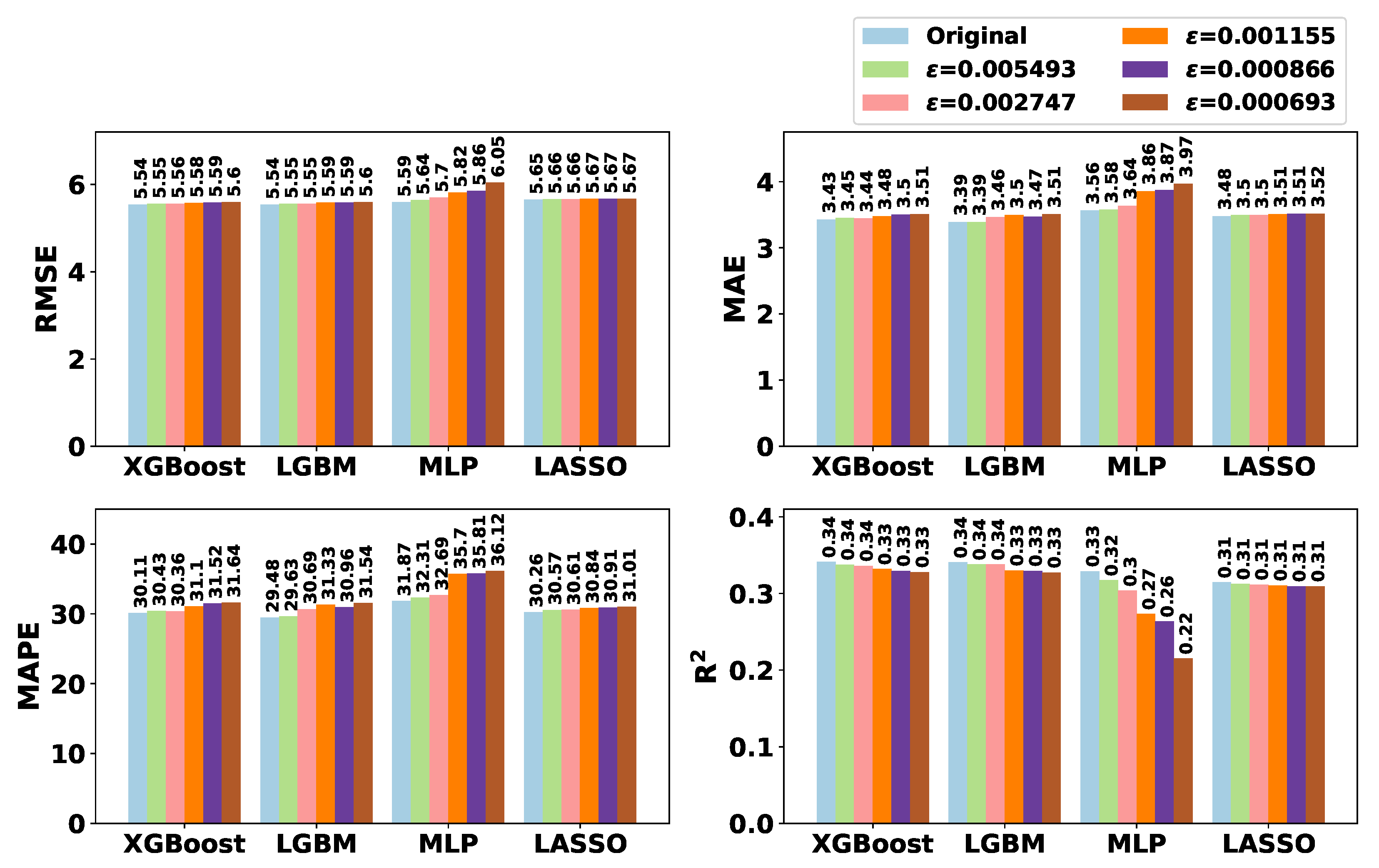
Figure 4 illustrates the impact of the level of GI for each ML model to predict ART according to each metric. As one can notice in this figure, for XGBoost, LGBM, and LASSO, there were minor differences between training models with original location data or sanitized ones. On the other hand, models trained with MLP performed poorly with GI-based data. In addition, by analyzing models trained with original data, while the smaller RMSE for LASSO is about 5.65, for more complex ML-based models, RMSE is less than 5.6, achieving 5.54 with XGBoost and LGBM. In comparison with the results of existing literature, lower R 2 scores and similar RMSE and MAE results were achieved in [11] to predict ART while using original location data only. With more details, Table A2 in Appendix A numerically exhibits the results from Figure 4.
Indeed, among the four tested models, LGBM and XGBoost achieve similar metric results while favoring the LGBM model. Thus, 
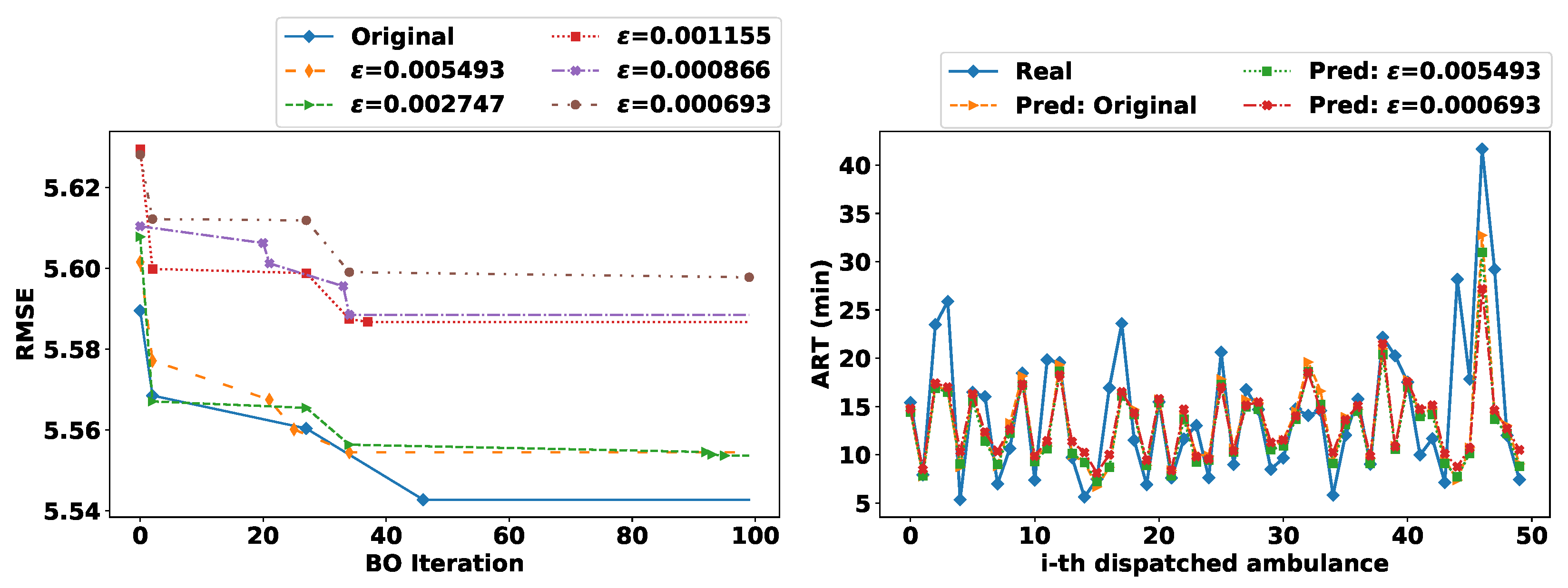
Figure 5 illustrates the BO iterative process for LGBM models trained with original and sanitized data according to the RMSE metric (left-hand plot); and ART prediction results for 50 dispatched ambulances in 2020 out of 8709 ones (right-hand plot) with an LGBM model trained with original data (Pred: original) and with two LGBM models trained sanitized data, i.e., with ϵ = 0.005493 (low privacy level) and with ϵ = 0.000693 (high privacy level).
As one can notice in the left-hand plot of Figure 5, once data are sanitized with different levels of ϵ -GI, the hyperparameters optimization via BO is also perturbed. This way, local minimums were achieved in different steps of the BO (i.e., the last marker per curve indicates the local minimum). For instance, even though ϵ = 0.002747 is stricter than ϵ = 0.005493 , results were still better for the former since, in the last steps of BO, three better local minimums were found. Moreover, prospective predictions were achieved with either original or sanitized data. For instance, in the right-hand plot of Figure 5, even for the high peak-value of ART around 40 min, LGBM’s prediction achieved some reasonable estimation. Although several features were perturbed due to the sanitization of the emergency scene (e.g., city, zone, etc.), the models could still achieve similar predictions as the model trained with original location data.
Furthermore, in terms of training time, for both original and sanitized datasets, the LASSO method was the fastest to fit our data. On the other hand, MLP models took the longest time to execute than all other methods. Between both decision-tree methods, LGBM models were faster than XGBoost ones. Lastly, the importance of the features, taking into account LASSO coefficients and decision trees’ importance scores were: averaged ART per categorical features (e.g., center, city, hour); OSRM API-based features (i.e., estimated driving distance and estimated travel time); the great-circle distance between the center and the emergency scene; the number of interventions in the previous hour, and the number of interventions still active. Immediately thereafter, it appeared the weather data, which were added as “real-time” features, i.e., using the date of the intervention to retrieve the features. Penultimate, the traffic data, which are indicators provided by [31] at the beginning of each year and, which might have shown more influence if they had been retrieved in real time. Finally, it appeared some temporal variables such as weekend indicators, start/end of the month, and the day of the year.

3.2. Discussion

The medical literature has mainly focused attention on the analysis of ART [3,34,43] and its association with trauma [2,30] and cardiac arrest [1,4,6], for example. To reduce ART, some works propose reallocation of ambulances [5,44], operation demand forecasting [5,7,8,22,45], travel time prediction [12], simulation models [35,46], and EMS response time predictions [11,12]. The work in [11] propose a real-time system for predicting ARTs for the San Francisco fire department, which closely relates to this paper. The authors processed about 4.5 million EMS calls using original location data to predict ART using four ML models, namely linear regression, linear regression with elastic net regularization, decision-tree regression, and random forest. However, no privacy-preserving experiment was performed because the main objective of their paper was proposing a scalable, ML-based, and real-time system for predicting ART. Besides, we also included weather data that the authors in [11] did not consider in their system, which could help to recognize high ARTs due to bad weather conditions, for example.
Currently, many private and public organizations collect and analyze data about their associates, customers, and patients. Because most of these data are personal and confidential (e.g., location), there is a need for privacy-preserving techniques for processing and using these data. Location privacy is an emergency research topic [13,14] due to the ubiquity of LBSs. Within our context, using and/or sharing the exact location of an emergency raises many privacy issues. For instance, the Seattle Fire Department [47] displays live EMS response information with the precise location and reason for the incident. Although the intention of some fire departments [11,47] is laudable, there are many ways for (mis)using this information, which can jeopardize users’ privacy. Even if the intervention’s 
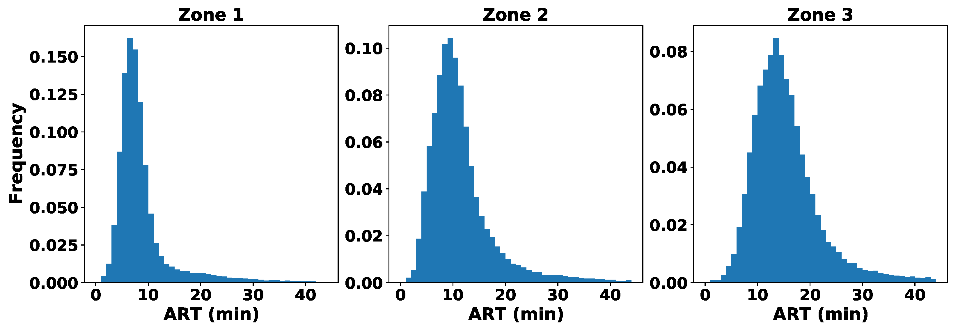
reason could be an indicator of the call urgency, we did not consider this sensitive attribute in our data analysis nor privacy-preserving prediction models. This is because, for SDIS 25, the ARTs limits are defined by the zone [9]. Additionally, we also did not include the victims’ personal data (e.g., gender, age) in our predictions or analysis since, during the calls, the operator may not acquire such information, e.g., when a third party activates the SDIS 25 for unidentified victims. This way, we focused our attention on the location privacy of each intervention.
To address location privacy, the authors in [15] proposed the concept of GI, which is based on a generalization [29] of the state-of-the-art DP [16] model. As highlighted in [
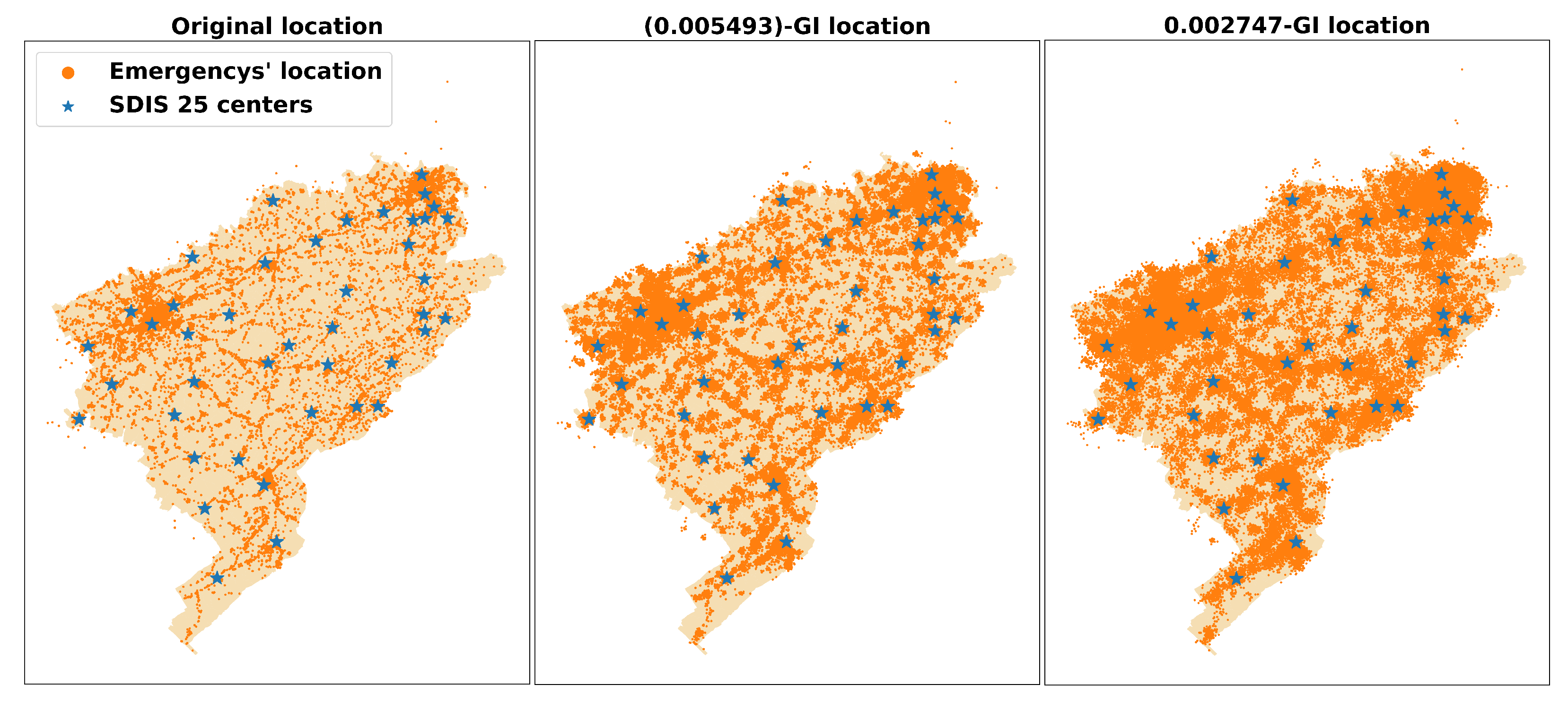
15], attackers in LSBs may have side information about the user’s reported location, e.g., knowing that the user is probably visiting the Eiffel Tower instead of swimming in the Seine river. However, this does not apply in our context because someone may have drowned, and EMS had to intervene. Similarly, even for the dataset with intermediate (and high) privacy in which locations are spread out in the Doubs region (cf. map with 0.005493 -GI location in Figure 3), someone may have been lost in the forest and EMS would have to interfere. For these reasons, using (or sharing datasets with) approximate emergency locations (e.g., sanitized with GI) is a prospective direction since many locations are possible emergency scenes. Indeed, we are not interested in hiding the emergency’s location completely since some approximate information is required to retrieve other features (e.g., city, zone, estimated distance) to use for predicting ART.
Moreover, learning and extracting meaningful patterns from data, e.g., through ML, play a key role in advancing and understanding several behaviors. However, on the one hand, storing and/or sharing original personal data with trusted curators may still lead to data breaches [48] and/or misuse of data, which compromises users’ privacy. On the other hand, training ML models with original data can also leak private information. For instance, in [18] the authors evaluate how some models can memorize sensitive information from the training data, and in [19], the authors investigate how ML models are susceptible to membership inference attacks. To address these problems, some works [7,20,21,22,23,24,25,49] propose to train ML models with sanitized data, which is also known as input perturbation [26] in the privacy-preserving ML literature.
Input perturbation-based ML and GI are linked directly with local DP [26] in which each sample is sanitized independently, either by the user during the data collection process or by the trusted curator, which aims to preserve privacy of each data sample. This way, data are protected from data leakage and are more difficult to reconstruct, for example. In [23,49], the authors investigate how input perturbation through applying controlled Gaussian noise on data samples can guarantee ( ϵ , δ ) -DP on the final ML model. This means, since ML models are trained with perturbed data, there is a perturbation on the gradient and on the final parameters of the model too.
In this paper, rather than Gaussian noise, the emergency scenes were sanitized with Algorithm 1, i.e., adding two-dimensional Laplacian noise centered at the exact user location x R 2 . In addition, this sanitization also perturbs other associated and calculated features such as: city, district, zone (e.g., urban or not), great-circle distance, estimated driving distance, and estimated travel time (cf. Table 3). As well as the optimization of hyperparameters, i.e., once data are differentially private, one can apply any function on it and, therefore, we also noticed perturbation on the BO procedure. Yet, as shown in the results, prospective ART predictions were achieved with either original or sanitized data. Furthermore, even with a high level of sanitization ( ϵ = 0.000693 ) there was a good privacy-utility trade-off. According to [50], if the mean absolute percentage error (i.e., MAPE) is greater than 20% and less than 50%, the forecast is reasonable, which is the results we have in this paper with MAPE around 30%.
Lastly, some limitations of this work are described in the following. We analyzed ARTs using the data and operation procedures of only one EMS in France, namely SDIS 25. Although it may represent a sufficient number of samples, other public and private organizations are also responsible for EMS calls, e.g., the SAMU (Urgent Medical Aid Service in English) analyzed in [46]. Moreover, there is the possibility of human error when using the mechanical system to report (i.e., record) the arrival on-scene time “ADate”. For instance, the crew may have forgotten to record status on arrival and may have registered later, or conversely, where the crew may have accidentally recorded before arriving at the location. Additionally, it is noteworthy to mention that the arrival on-scene does not mean arriving at the victim’s side, e.g., in some cases the real location of a victim is at the n-th stage of a building as investigated in [43].

4. Conclusions

In the event of an acute medical event such as a respiratory crisis or cardio-respiratory arrest, the time an ambulance takes to arrive on-scene has a direct impact on the quality of service provided. Ambulance response time is a fundamental indicator of the effectiveness of EMS systems [1,2,4,5,6,30]. For this reason, an intelligent decision-support system is necessary to help minimize overall EMS response times. The present work first analyzes historical records of ARTs to find correlations between their extracted features and explain the trends through the 15 years of collected data. Then, we sought to predict the response time that each center equipped with ambulances had to an event, but not only that, because we also consider that the ML models could be subject to attacks, which would compromise the victims’ privacy. Therefore, the joint work aimed to evaluate the effectiveness of predicting ARTs with ML models trained over sanitized location data with different levels of ϵ -geo-indistinguishability. As shown in the results, the sanitization of location data and the perturbation of its associated features (e.g., city, distance) had no considerable impact on predicting ART. With these findings, EMS may prefer using and/or sharing sanitized datasets to avoid possible data leakages, membership inference attacks, or data reconstructions, for example.
For future work, we aim to extend the analysis and predictions to different operation times such as the pre-travel delay (i.e., gathering personnel and ambulances) and travel times (e.g., from the center to the emergency scene, from the emergency scene to hospitals), while respecting users’ privacy. In addition, new variables will be added such as the number of dispatched ambulances registered in a previous or current time, and the number of ambulances and firefighters available in each center at a given time, given that while there are few resources available, ART may be longer. Indeed, the aim is to build an intelligent system capable of predicting ARTs while respecting victims’ privacy. This way, this system would allow reinforcing SDIS 25 centers with the necessary firefighters to attend incidents faster; to create a new center according to the concurrence and high average ARTs for a given area; as well as to convert a static resource deployment plan into a dynamic one, which would be based on the selection of the center with shorter response times taking into account the community the emergency took place, traffic and weather conditions, and so on. Lastly, we would like to evaluate, in practice, the trade-off between such an ART prediction decision-support system with the victims’ privacy, on using ϵ -GI location data.

Author Contributions

Conceptualization, H.H.A. and S.C.; methodology, H.H.A. and S.C.; software, H.H.A. and S.C.; validation, H.H.A. and S.C.; formal analysis, H.H.A. and S.C.; investigation, H.H.A., S.C., C.G., and J.-F.C.; resources, C.G. and J.-F.C.; data curation, H.H.A. and S.C.; writing—original draft preparation, H.H.A., S.C., C.G., and J.-F.C.; writing—review and editing, H.H.A., S.C., C.G., and J.-F.C.; visualization, S.C. and C.G.; supervision, C.G. and J.-F.C.; project administration, C.G. and J.-F.C.; funding acquisition, C.G. and J.-F.C. All authors have read and agreed to the published version of the manuscript.

Funding

This research received no external funding.

Acknowledgments

This work was supported by the Region of Bourgogne Franche-Comté CADRAN Project, by the EIPHI-BFC Graduate School (contract “ANR-17-EURE-0002”), and by SDIS du Doubs, with the support of the French Ministry of Higher Education and Research (managed by the National Association of Research and Technology (ANRT) for the CIFRE thesis (N 2019/0372). The authors would also like to thank SDIS 25 Commander Guillaume Royer-Fey and Captain Céline Chevallier for their great collaborations and continuous feedback. All computations have been performed on the “Mésocentre de Calcul de Franche-Comté”.

Conflicts of Interest

The authors declare no conflict of interest.

Abbreviations

The following abbreviations are used in this manuscript:
ARTAmbulance response time
BOBayesian optimization
DPDifferential privacy
EMSEmergency medical services
GIGeo-Indistinguishability
LASSOLeast Absolute Shrinkage and Selection Operator
LBSsLocation-based services
LDPLocal differential privacy
LGBMLight Gradient Boosted Machine
MLPMultilayer Perceptron
MAEMean absolute error
MAPEMean absolute percentage error
RMSERoot mean squared error
SDIS 25Departmental Fire and Rescue Service of Doubs
XGBoostExtreme Gradient Boosting
Z1Zone urban
Z2Zone semi-urban
Z3Zone rural

Appendix A. Complementary Results

Table A1. Search space for hyperparameters by ML model and the best configuration obtained for predicting ARTs per dataset.
ModelSearch SpaceBest Configuration per Dataset
Original ϵ = 0.005493 ϵ = 0.002747 ϵ = 0.001155 ϵ = 0.000866 ϵ = 0.000693
XGBoostmax_depth: [1, 10]996699
n_estimators: [50, 500]465465130235465465
learning_rate: [0.001, 0.5]0.02650.02650.08580.04860.02650.0265
min_child_weight: [1, 10]557755
max_delta_step: [1, 11]443444
gamma: [0.5, 5]330233
subsample: [0.5, 1]0.80.8110.80.8
colsample_bytree: [0.5, 1]0.50.50.50.50.50.5
alpha: [0, 5]221222
LGBMmax_depth: [1, 10]7810886
n_estimators: [50, 500]35532647725080441
learning_rate: [1 × 10 4 , 0.5]0.01880.00980.01640.02850.05860.0300
subsample: [0.5, 1]0.540660.52280.61380.66990.67320.5812
colsample_bytree: [0.5, 1]0.51600.55750.52040.68700.55070.5451
num_leaves: [31, 400]40019224539813295
reg_alpha: [0, 5]405014
MLPDense layers: [1, 7]734666
Number of neurons: [ 2 8 , 2 13 ] 2 10 2 12 2 12 2 9 2 12 2 9
Batch size: [32, 168]1408048827044
Learning rate: [1 × 10 5 , 0.01]0.002650.001240.00990.00990.00940.0077
Optimizer: AdamAdamAdamAdamAdamAdamAdam
Epochs: 100100100100100100100
Early stopping: 10101010101010
LASSOalpha: [0.01, 2]0.02050.03070.01050.01000.01120.0107
Table A2. Metrics results for each ML model trained with original data and sanitized ones.
DataMetricXGBoostLGBMMLPLASSO
OriginalRMSE5.53985.54275.59165.6511
MAE3.42863.38803.56233.4760
MAPE30.11429.47631.86730.260
R 2 0.34120.34050.32890.3145
ϵ = 0.005493 RMSE5.55475.55445.64015.6596
MAE3.45153.39153.57733.4960
MAPE30.43229.62832.30730.571
R 2 0.33770.33780.31720.3124
ϵ = 0.002747 RMSE5.56175.55365.69595.6636
MAE3.44303.46283.63573.4991
MAPE30.36430.68832.68730.606
R 2 0.33600.33790.30360.3115
ϵ = 0.001155 RMSE5.57885.58675.81845.6671
MAE3.48033.49913.85503.5094
MAPE31.09731.32735.70430.835
R 2 0.33190.33000.27330.3106
ϵ = 0.000866 RMSE5.58925.58855.85755.6716
MAE3.50333.47023.87363.5134
MAPE31.51530.96435.81030.907
R 2 0.32950.32960.26350.3095
ϵ = 0.000693 RMSE5.59625.59786.04635.6717
MAE3.51193.50873.97043.5171
MAPE31.63831.54336.12231.007
R 2 0.32780.32740.21530.3095

References

  1. Bürger, A.; Wnent, J.; Bohn, A.; Jantzen, T.; Brenner, S.; Lefering, R.; Seewald, S.; Gräsner, J.T.; Fischer, M. The Effect of Ambulance Response Time on Survival Following Out-of-Hospital Cardiac Arrest. Deutsches Aerzteblatt Online 2018. [Google Scholar] [CrossRef]
  2. Byrne, J.P.; Mann, N.C.; Dai, M.; Mason, S.A.; Karanicolas, P.; Rizoli, S.; Nathens, A.B. Association Between Emergency Medical Service Response Time and Motor Vehicle Crash Mortality in the United States. JAMA Surg. 2019, 154, 286. [Google Scholar] [CrossRef] [PubMed]
  3. Do, Y.K.; Foo, K.; Ng, Y.Y.; Ong, M.E.H. A Quantile Regression Analysis of Ambulance Response Time. Prehosp. Emerg. Care 2012, 17, 170–176. [Google Scholar] [CrossRef] [PubMed]
  4. Holmén, J.; Herlitz, J.; Ricksten, S.E.; Strömsöe, A.; Hagberg, E.; Axelsson, C.; Rawshani, A. Shortening Ambulance Response Time Increases Survival in Out-of-Hospital Cardiac Arrest. J. Am. Heart Assoc. 2020, 9. [Google Scholar] [CrossRef] [PubMed]
  5. Chen, A.Y.; Lu, T.Y.; Ma, M.H.M.; Sun, W.Z. Demand Forecast Using Data Analytics for the Preallocation of Ambulances. IEEE J. Biomed. Health Inform. 2016, 20, 1178–1187. [Google Scholar] [CrossRef] [PubMed]
  6. Lee, D.W.; Moon, H.J.; Heo, N.H. Association between ambulance response time and neurologic outcome in patients with cardiac arrest. Am. J. Emerg. Med. 2019, 37, 1999–2003. [Google Scholar] [CrossRef] [PubMed]
  7. Arcolezi, H.H.; Couchot, J.F.; Cerna, S.; Guyeux, C.; Royer, G.; Bouna, B.A.; Xiao, X. Forecasting the number of firefighter interventions per region with local-differential-privacy-based data. Comput. Secur. 2020, 96, 101888. [Google Scholar] [CrossRef]
  8. Cerna, S.; Guyeux, C.; Arcolezi, H.H.; Couturier, R.; Royer, G. A Comparison of LSTM and XGBoost for Predicting Firemen Interventions. In Trends and Innovations in Information Systems and Technologies; Springer International Publishing: Cham, Switzerland, 2020; pp. 424–434. [Google Scholar] [CrossRef]
  9. Cerna, S.; Guyeux, C.; Royer, G.; Chevallier, C.; Plumerel, G. Predicting Fire Brigades Operational Breakdowns: A Real Case Study. Mathematics 2020, 8, 1383. [Google Scholar] [CrossRef]
  10. Nehme, Z.; Andrew, E.; Smith, K. Factors Influencing the Timeliness of Emergency Medical Service Response to Time Critical Emergencies. Prehosp. Emerg. Care 2016, 20, 783–791. [Google Scholar] [CrossRef]
  11. Lian, X.; Melancon, S.; Presta, J.R.; Reevesman, A.; Spiering, B.; Woodbridge, D. Scalable Real-Time Prediction and Analysis of San Francisco Fire Department Response Times. In Proceedings of the 2019 IEEE SmartWorld, Ubiquitous Intelligence & Computing, Advanced & Trusted Computing, Scalable Computing & Communications, Cloud & Big Data Computing, Internet of People and Smart City Innovation (SmartWorld/SCALCOM/UIC/ATC/CBDCom/IOP/SCI), Leicester, UK, 19–23 August 2019. [Google Scholar] [CrossRef]
  12. Aladdini, K. EMS Response Time Models: A Case Study and Analysis for the Region of Waterloo. Master’s Thesis, University of Waterloo, Waterloo, ON, Canada, 2010. [Google Scholar]
  13. Shokri, R.; Theodorakopoulos, G.; Boudec, J.Y.L.; Hubaux, J.P. Quantifying Location Privacy. In Proceedings of the 2011 IEEE Symposium on Security and Privacy, Oakland, CA, USA, 22–25 May 2011. [Google Scholar] [CrossRef] [Green Version]
  14. Chatzikokolakis, K.; ElSalamouny, E.; Palamidessi, C.; Pazii, A. Methods for Location Privacy: A comparative overview. Found. Trends Priv. Secur. 2017, 1, 199–257. [Google Scholar] [CrossRef]
  15. Andrés, M.E.; Bordenabe, N.E.; Chatzikokolakis, K.; Palamidessi, C. Geo-indistinguishability. In Proceedings of the 2013 ACM SIGSAC Conference on Computer & Communications Security, Berlin, Germany, 4–8 November 2013. [Google Scholar] [CrossRef] [Green Version]
  16. Dwork, C.; Roth, A. The algorithmic foundations of differential privacy. Found. Trends Theor. Comput. Sci. 2014, 9, 211–407. [Google Scholar] [CrossRef]
  17. Location Guard. Available online: https://github.com/chatziko/location-guard (accessed on 2 August 2021).
  18. Song, C.; Ristenpart, T.; Shmatikov, V. Machine Learning Models that Remember Too Much. In Proceedings of the 2017 ACM SIGSAC Conference on Computer and Communications Security, Dallas, TX, USA, 30 October–3 November 2017. [Google Scholar] [CrossRef] [Green Version]
  19. Shokri, R.; Stronati, M.; Song, C.; Shmatikov, V. Membership Inference Attacks Against Machine Learning Models. In Proceedings of the 2017 IEEE Symposium on Security and Privacy, San Jose, CA, USA, 22–24 May 2017. [Google Scholar] [CrossRef] [Green Version]
  20. Chamikara, M.A.P.; Bertok, P.; Khalil, I.; Liu, D.; Camtepe, S. Privacy Preserving Face Recognition Utilizing Differential Privacy. Comput. Secur. 2020, 97, 101951. [Google Scholar] [CrossRef]
  21. Fan, L. Image Pixelization with Differential Privacy. In Proceedings of the 32nd IFIP Annual Conference on Data and Applications Security and Privacy, Bergamo, Italy, 16–18 July 2018; pp. 148–162. [Google Scholar] [CrossRef]
  22. Couchot, J.F.; Guyeux, C.; Royer, G. Anonymously forecasting the number and nature of firefighting operations. In Proceedings of the 23rd International Database Applications & Engineering Symposium, Athens, Greece, 10–12 June 2019. [Google Scholar] [CrossRef]
  23. Fukuchi, K.; Tran, Q.K.; Sakuma, J. Differentially Private Empirical Risk Minimization with Input Perturbation. In Proceedings of the International Conference on Discovery Science, Kyoto, Japan, 15–17 October 2017; pp. 82–90. [Google Scholar] [CrossRef] [Green Version]
  24. Agrawal, D.; Aggarwal, C.C. On the design and quantification of privacy preserving data mining algorithms. In Proceedings of the Twentieth ACM SIGMOD-SIGACT-SIGART Symposium on Principles of Database Systems, Santa Barbara, CA, USA, 21–23 May 2001. [Google Scholar] [CrossRef]
  25. Agrawal, R.; Srikant, R. Privacy-preserving data mining. In Proceedings of the 2000 ACM SIGMOD International Conference on Management of Data, Dallas, TX, USA, 15–18 May 2000. [Google Scholar] [CrossRef]
  26. Kasiviswanathan, S.P.; Lee, H.K.; Nissim, K.; Raskhodnikova, S.; Smith, A. What Can We Learn Privately? In Proceedings of the 2008 49th Annual IEEE Symposium on Foundations of Computer Science, Philadelphia, PA, USA, 26–28 October 2008. [Google Scholar] [CrossRef] [Green Version]
  27. Chaudhuri, K.; Monteleoni, C.; Sarwate, A.D. Differentially private empirical risk minimization. J. Mach. Learn. Res. 2011, 12, 1069–1109. [Google Scholar] [PubMed]
  28. Abadi, M.; Chu, A.; Goodfellow, I.; McMahan, H.B.; Mironov, I.; Talwar, K.; Zhang, L. Deep Learning with Differential Privacy; Association for Computing Machinery: New York, NY, USA, 2016; pp. 308–318. [Google Scholar] [CrossRef] [Green Version]
  29. Chatzikokolakis, K.; Andrés, M.E.; Bordenabe, N.E.; Palamidessi, C. Broadening the Scope of Differential Privacy Using Metrics. In Privacy Enhancing Technologies; Springer: Berlin/Heidelberg, Germany, 2013; pp. 82–102. [Google Scholar] [CrossRef] [Green Version]
  30. Pons, P.T.; Markovchick, V.J. Eight minutes or less: Does the ambulance response time guideline impact trauma patient outcome? J. Emerg. Med. 2002, 23, 43–48. [Google Scholar] [CrossRef]
  31. Bison-Futé. Les Prévisions de Trafic. Available online: https://www.bison-fute.gouv.fr (accessed on 2 February 2021).
  32. Météo-France. Données Publiques. Available online: https://donneespubliques.meteofrance.fr/?fond=produit&id_produit=90&id_rubrique=32 (accessed on 2 February 2021).
  33. Luxen, D.; Vetter, C. Real-time routing with OpenStreetMap data. In Proceedings of the 19th ACM SIGSPATIAL International Conference on Advances in Geographic Information Systems, Chicago, IL, USA, 1–4 November 2011; pp. 513–516. [Google Scholar] [CrossRef]
  34. Austin, P.C. Quantile Regression: A Statistical Tool for Out-of-Hospital Research. Acad. Emerg. Med. 2003, 10, 789–797. [Google Scholar] [CrossRef]
  35. Peleg, K.; Pliskin, J.S. A geographic information system simulation model of EMS: Reducing ambulance response time. Am. J. Emerg. Med. 2004, 22, 164–170. [Google Scholar] [CrossRef]
  36. Chen, T.; Guestrin, C. XGBoost: A Scalable Tree Boosting System. In Proceedings of the 22nd ACM SIGKDD International Conference on Knowledge Discovery and Data Mining, San Francisco, CA, USA, 13–17 August 2016. [Google Scholar] [CrossRef] [Green Version]
  37. Ke, G.; Meng, Q.; Finley, T.; Wang, T.; Chen, W.; Ma, W.; Ye, Q.; Liu, T.Y. LightGBM: A Highly Efficient Gradient Boosting Decision Tree. In Advances in Neural Information Processing Systems 30; Guyon, I., Luxburg, U.V., Bengio, S., Wallach, H., Fergus, R., Vishwanathan, S., Garnett, R., Eds.; Curran Associates, Inc.: Red Hook, NY, USA, 2017; pp. 3146–3154. [Google Scholar]
  38. Goodfellow, I.; Bengio, Y.; Courville, A.; Bengio, Y. Deep Learning; MIT Press: Cambridge, MA, USA, 2016; Volume 1. [Google Scholar]
  39. Keras. Available online: https://keras.io (accessed on 2 August 2021).
  40. Tibshirani, R. Regression Shrinkage and Selection via the Lasso. J. R. Stat. Soc. B Methodol. 1996, 58, 267–288. [Google Scholar] [CrossRef]
  41. Pedregosa, F.; Varoquaux, G.; Gramfort, A.; Michel, V.; Thirion, B.; Grisel, O.; Blondel, M.; Pedregosa, P.; Weiss, R.; Dubourg, V.; et al. Scikit-learn: Machine Learning in Python. J. Mach. Learn. Res. 2011, 12, 2825–2830. [Google Scholar]
  42. Bergstra, J.; Yamins, D.; Cox, D.D. Making a Science of Model Search: Hyperparameter Optimization in Hundreds of Dimensions for Vision Architectures. In Proceedings of the 30th International Conference on International Conference on Machine Learning, Atlanta, GA, USA, 16–21 June 2013; pp. I-115–I-123. [Google Scholar]
  43. Silverman, R.A.; Galea, S.; Blaney, S.; Freese, J.; Prezant, D.J.; Park, R.; Pahk, R.; Caron, D.; Yoon, S.; Epstein, J.; et al. The “Vertical Response Time”: Barriers to Ambulance Response in an Urban Area. Acad. Emerg. Med. 2007, 14, 772–778. [Google Scholar] [CrossRef]
  44. Carvalho, A.; Captivo, M.; Marques, I. Integrating the ambulance dispatching and relocation problems to maximize system’s preparedness. Eur. J. Oper. Res. 2020, 283, 1064–1080. [Google Scholar] [CrossRef]
  45. Lin, A.X.; Ho, A.F.W.; Cheong, K.H.; Li, Z.; Cai, W.; Chee, M.L.; Ng, Y.Y.; Xiao, X.; Ong, M.E.H. Leveraging Machine Learning Techniques and Engineering of Multi-Nature Features for National Daily Regional Ambulance Demand Prediction. Int. J. Environ. Res. Public Health 2020, 17, 4179. [Google Scholar] [CrossRef] [PubMed]
  46. Aboueljinane, L.; Jemai, Z.; Sahin, E. Reducing ambulance response time using simulation: The case of Val-de-Marne department Emergency Medical service. In Proceedings of the 2012 Winter Simulation Conference (WSC), Berlin, Germany, 9–12 December 2012. [Google Scholar] [CrossRef]
  47. Seattle Fire Department: Real-Time 911 Dispatch. Available online: http://www2.seattle.gov/fire/realtime911/ (accessed on 18 February 2021).
  48. McCandless, D.; Evans, T.; Quick, M.; Hollowood, E.; Miles, C.; Hampson, D.; Geere, D. World’s Biggest Data Breaches & Hacks. 2021. Available online: https://www.informationisbeautiful.net/visualizations/worlds-biggest-data-breaches-hacks/ (accessed on 18 February 2021).
  49. Kang, Y.; Liu, Y.; Niu, B.; Tong, X.; Zhang, L.; Wang, W. Input Perturbation: A New Paradigm between Central and Local Differential Privacy. arXiv 2020, arXiv:2002.08570. [Google Scholar]
  50. Lewis, C. Industrial and Business Forecasting Methods: A Practical Guide to Exponential Smoothing and Curve Fitting; Butterworth Scientific: London, UK, 1982. [Google Scholar]
Figure 1. Distribution of the ART variable for zones Z1, Z2, and Z3, respectively.
Mca 26 00056 g001
Figure 2. Histogram of the total number of dispatched ambulances per hour in the day (left-hand plot) and cumulative ART in hours per day of the week and hour in the day (right-hand plot).
Mca 26 00056 g002
Figure 3. Emergency locations and SDIS 25 centers throughout the Doubs region: original data (left-hand plot), ϵ = 0.005493 -GI data (middle plot), and ϵ = 0.002747 -GI data (right-hand plot).
Mca 26 00056 g003
Figure 4. Impact of the level of ϵ -geo-indistinguishability for each ML model to predict ART according to each metric.
Mca 26 00056 g004
Figure 5. The left-hand plot illustrates the hyperparameters tuning process via Bayesian optimization with 100 iterations for LGBM models trained with original data and sanitized ones. The right-hand plot illustrates the prediction of ARTs with LGBM models trained with original data and with sanitized ones.
Mca 26 00056 g005
Table 1. Mean and std values for the ART variable and the total number of dispatched ambulances (Nb. Amb.) per year in zones Z1, Z2, and Z3, respectively. For 2020, we only consider cases of the first semester.
YearZ1Z2Z3
Nb. Amb.MeanStdNb. Amb.MeanStdNb. Amb.MeanStd
20061979.234.4136711.255.5035414.275.40
20072367.393.0567110.795.0459514.355.52
20087998.696.04105511.195.3291114.536.02
200913638.766.05208711.085.67187214.946.46
2010264310.087.23279712.486.85248316.017.22
201159718.265.61427611.246.13329514.506.25
201260788.665.89466111.186.39360214.866.24
201367808.825.72504811.036.11397215.076.30
201468478.375.23548110.805.86424014.916.34
201572268.465.50559610.865.78464315.026.12
201675108.505.35617911.195.92486115.326.35
201786508.765.32725111.496.01552315.516.36
201890518.905.46764111.646.11595615.596.23
201970309.426.02623812.296.66501616.606.88
202033979.735.87284312.596.56244916.466.44
Table 2. Values of ϵ = l / r for sanitizing emergency location data with GI.
ϵ = l / r lr (m)
0.005493 ln ( 3 ) 200
0.002747 ln ( 3 ) 400
0.001155 ln ( 2 ) 600
0.000866 ln ( 2 ) 800
0.000693 ln ( 2 ) 1000
Table 3. Percentage of perturbation for categorical attributes (city, zone, and district) according to ϵ and statistical properties (mean and std values and correlation with ART) of the original and GI-based datasets for the great-circle distance attribute. Mean(std) values are reported since we repeated our experiments with 10 different seeds.
DataZoneCityDistrictGreat-Circle Dist. (km)
‘Perturbation’ (%)MeanstdCorr. ART
Original---3.443.720.369
ϵ = 0.005493 5.20 (0.05)7.68 (0.06)25.8 (0.05)3.48 (1 × 10 3 )3.72 (7 × 10 4 )0.367 (2 × 10 4 )
ϵ = 0.002747 11.3 (0.05)17.6 (0.10)41.5 (0.12)3.57 (1 × 10 3 )3.72 (1 × 10 3 )0.362 (2 × 10 4 )
ϵ = 0.001155 28.1 (0.06)42.3 (0.10)66.2 (0.09)4.03 (3 × 10 3 )3.74 (3 × 10 3 )0.335 (5 × 10 4 )
ϵ = 0.000866 35.5 (0.10)52.4 (0.11)74.0 (0.11)4.38 (3 × 10 3 )3.81 (4 × 10 3 )0.313 (1 × 10 3 )
ϵ = 0.000693 41.4 (0.12)60.3 (0.09)79.4 (0.05)4.77 (6 × 10 3 )3.92 (5 × 10 3 )0.288 (1 × 10 3 )
Publisher’s Note: MDPI stays neutral with regard to jurisdictional claims in published maps and institutional affiliations.

