Article

Prediction of Bleeding via Simulation of Hydrodynamics in Centrifugal Partition Chromatography

Laboratory of Plant and Process Design, Department of Biochemical and Chemical Engineering, TU Dortmund University, 44227 Dortmund, Germany
*
Author to whom correspondence should be addressed.
Separations 2024, 11(1), 16; https://doi.org/10.3390/separations11010016
Submission received: 23 November 2023 / Revised: 22 December 2023 / Accepted: 28 December 2023 / Published: 3 January 2024

Abstract

:
Centrifugal Partition Chromatography (CPC) utilizes a two-phase liquid–liquid system as mobile and stationary phases. During operation, the latter continuously drains out of the rotor, despite it being in fact stationary, leading to decreasing separation efficiency over time, a phenomenon still poorly understood today because neither simulations nor extensive experimental investigations have addressed this so-called bleeding. With the model presented in this study, the underlying hydrodynamics are discussed in detail. This model can simulate bleeding over 60 s and is verified experimentally for different operating points (volumetric flow rates of 5, 12, and 20 mL⋅min−1) of the Centrifugal Partition Chromatograph utilizing an aqueous–organic phase system. We simulated two interconnected chambers at the rotor inlet and analyzed the loss of the stationary phase over time. The results of the simulated second chamber are closely aligned with the experimental validation results. Thus, the prediction of bleeding utilizing the simulation of hydrodynamics was successful. Moreover, we highlighted the benefits of the two-chamber setup modeled in this study compared to single-chamber models.

1. Introduction

As the demand for sustainably produced biomolecules increases continually, so does the need for cost-efficient production. Because of the growing complexity of products, the focus is usually on maximizing product titers in upstream processing and fermentation. However, downstream processes are often not fully optimized or are incapable of handling the high product titers, causing up to 90% of production costs in extreme cases. The future scope of the market will be twofold: large-scale production on the one hand and flexible technologies for rapid development and efficient small-scale manufacturing on the other hand. Consequently, a profound understanding of all processes becomes more critical than ever [1,2]. Countercurrent Chromatography offers a well-fitting technique in terms of cost-effectiveness and flexibility. Hydrostatic and hydrodynamic Countercurrent Chromatography are the main technical concepts to differentiate [3]. The hydrostatic variant, also referenced as Centrifugal Partition Chromatography (CPC), is particularly interesting for industrial applications [4,5]. Its technical implementation is robust because hardly any wear and tear parts are needed, and the apparatus is not prone to leakages.
The underlying concept is a rotor with an embedded cascade of chambers and interconnecting channels. The rotor is flanged to an electric motor and spins typically at 500 to 2000 rounds per minute. This way, centrifugal forces immobilize one of the two liquid phases inside the chambers. That phase is called the stationary phase. Compared to other chromatographic techniques—for instance, High-Performance Liquid Chromatography (HPLC)—the stationary phase is not solid, implying several advantages.
As mentioned, costs are critical, and liquid stationary phases are significantly less expensive than solid ones [6,7]. Another advantage becomes apparent when considering the second phase involved, i.e., the mobile phase. As a crucial requirement is immiscibility, the emerging phase boundary between the mobile and stationary phase is the place of mass transfer. In reverse, the partition coefficient KD, which is comparatively easy to determine, is the driving force for mass transfer. That leads to precise predictability of the separation performance for different solvent systems [8,9,10,11]. Especially in bioprocess downstream engineering, sensitive products, such as proteins or antibodies, benefit from solvents providing mild conditions [12]. Studies proved that liquid–liquid chromatographic separation of antibodies (immunoglobulin Y) with the help of aqueous two-phase systems is possible [13]. Even multiphase enzymatic reactions were performed with the help of aqueous two-phase systems in a Centrifugal Partition Chromatograph [14,15].
Furthermore, solvent systems, i.e., ionic liquids and deep eutectic solvents, are of interest in Countercurrent Chromatography. With biphasic ionic liquids, a limiting constraint is their comparably high viscosity; the increased pressure in the chromatograph can limit the scale-up capabilities. Here, technical solutions have to be found. On the other hand, deep eutectic solvents are mainly used in combination with apolar solvents. The system’s polarity is adjustable with the help of solubilizers. This raises the relevance for Countercurrent Chromatography, as the partition coefficient for the samples of a given separation task becomes adjustable [16,17,18,19,20,21]. Further advantages are high loading capacities and total recovery of the products.
As mentioned, immobilization of the stationary phase occurs in the rotor chambers. The fluid is trapped inside those by a centrifugal field. During operation, the mobile phase is dispersed in the stationary phase at every chamber’s inlet and coalesces before exiting via the outgoing channel towards the next chamber [22]. Unfortunately, the liquid inside the coalescing zone always contains small amounts of stationary phase, i.e., the coalescence is imperfect. Thus, the stationary phase leaks continuously out of the apparatus—the so-called bleeding. Bleeding limits the operating period; in theory, performing a separation becomes impossible with the last drop of the stationary phase leaving the chromatograph. In practice, the rotor has to be filled with 20 vol% to 80 vol% of the stationary phase to maintain economically reasonable performance [6]. Many different chamber geometries were developed to achieve this, aiming for sufficient retention and good dispersion [23,24]. This task led to an extensive experimental effort in the past because different rotor geometries had to be manufactured and experiments covering several operating points had to be performed (i.e., different phase systems, volumetric flows, rpm) [25,26,27]. As a solution, Computational Fluid Dynamics (CFD) seems to provide a promising technique for gaining an in-depth understanding of the hydrodynamics involved. A time-dependent simulation should provide sufficient insight into the mechanisms of bleeding. Considering all three dimensions is a benefit over the (camera-based) two-dimensional information gained during experiments. In previous works, we addressed the simulation of hydrodynamic effects during startup (first 0.3 s of operation) [28]. In this work, however, the focus is on model bleeding over increased periods of time since this is needed to predict the bleeding behavior.

2. Materials and Methods

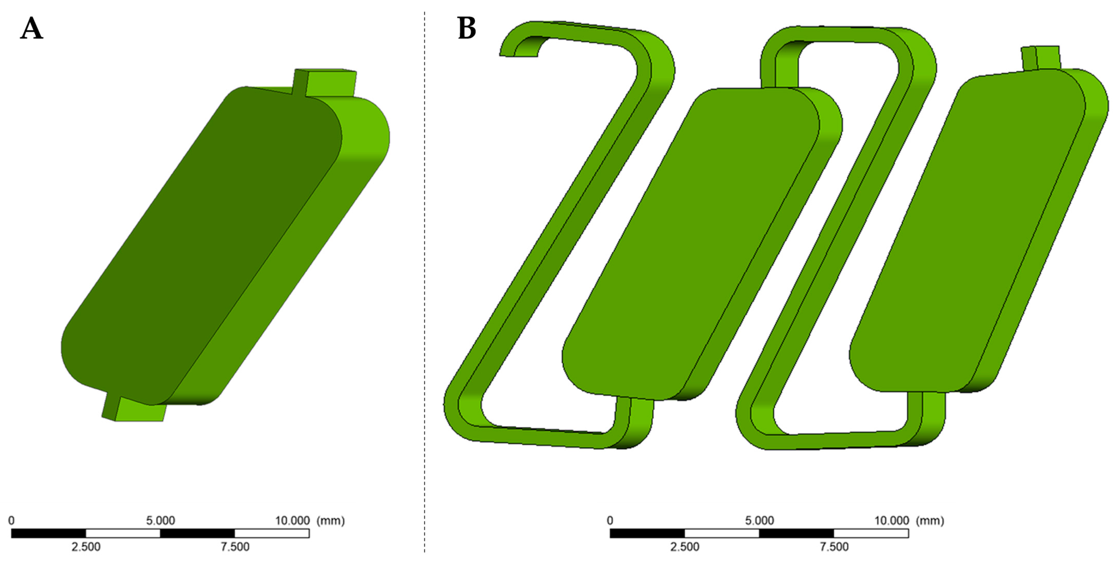
2.1. Model Generation

All simulations were performed using Ansys© 2021 R1 [29]. The calculations necessary were conducted at the Linux High-performance Computing Cluster LiDo 3 of TU Dortmund University. As a first step, the forces involved must be addressed. Due to the angular velocity ω , rotational forces impact the fluid inside the rotor. As a result, centrifugal acceleration a _ C f is present, resulting from the inertia of fluids (Equation (1)) [30].
a _ C f = ω _ × ω _ × r _
The direction of this acceleration is orthogonal to the axis of rotation, with r being the distance between this axis and the fluid volume considered. Because the setup acts like a rotating frame of reference, the inertial Coriolis acceleration a _ C o must also be taken into account (Equation (2)).
a _ C o = 2 · ω _ × u _
The acceleration is directed orthogonally to the velocity of the fluid element u . The respective forces are obtained by multiplying the accelerations with the fluid mass m (Equation (3)).
F _ r o t = m · a _ r o t
Those forces are schematically depicted in Figure 1.
The forces are implemented in a physical model. Therefore, terms for convective flow (Equation (4)), diffusive flow (Equation (5)), and source terms (Equations (6)–(8)), including the forces mentioned, are needed.
F φ = ρ u _ φ
D φ = Γ φ
S x = ρ m i x · x · 2 π · N t 2 + 2 · ρ m i x · v · 2 π · N t
S y = ρ m i x · y · 2 π · N t 2 2 · ρ m i x · u · 2 π · N t
S z = 0
Γ is the diffusion coefficient, ∆N·∆t−1 describes the revolutions per minute (rpm), while u and v form the velocity vector u _ . The assumption of an incompressible fluid can be made because the maximum pressure the apparatus can handle is 50 bar. With the phase systems used being Newtonian fluids, the shear stress τ _ is a function of the dynamic viscosity η [31,32]. Moreover, η and the density ρ depend on the phase described [33,34]. Isothermal operation is assumed, and the finite volume method (FVM) was applied for the numerical solution. This commonly used solution method divides the flow regime into control volumes (CV).
In the next step, a computational mesh is needed. The flow geometries to be analyzed are based on a modified FCPC-rotor (Kromaton, Annonay, France) [24]. The exact dimensions are shown in Figure 2.
The coordinate system used has its origin at r = 0. To keep the simulation effort at a reasonable level, a single chamber, including a short duct section at the inlet and outlet, was modeled at first. Next, we simulated fluid dynamics inside a two-chamber setup with interconnecting ducts (single-chamber and two-chamber setup (Figure A1)). Therefore, the spatial domain is discretized into a finite number of cells, forming a numerical grid. This grid represents the physical domain over which the problem is being solved. Each cell in the grid is typically assumed to have uniform properties, such as material properties, and the values of the solution variables are computed at the center of each cell. The method calculates the fluxes of these variables across the faces of the cells and uses these fluxes to update the values of the variables inside each cell [36].
A mesh independence study was performed to find the optimal mesh size. The characteristic variable was the averaged phase fraction α . The goal is to find a mesh size where the mesh resolution does not influence α . A hybrid mesh was created using the Ansys © ICEM CFD meshing tool (Available online: https://www.ansys.com/training-center/course-catalog/fluids/introduction-to-ansys-icem-cfd, accessed on 27 December 2023). The installation of a body-fitted mesh allowed for a high-quality approximation of all radii in the flow domain (i.e., rounded corners of the chamber). Structured rectangular patterns were used on all straight geometries. We utilized an orthogonal grid with an identical setup in each plane of the z-direction (height of chambers and channels). When interconnected with channels, those were meshed separately. We varied the maximum size of individual cells for the mesh independence study between 0.07 mm and 0.2 mm. The number of divisions along the z-axis was tested between 20 and 45 (Table A1).
Further settings regarding the simulation of multiphase flows were set [24,33,34]. We utilized the Volume of Fluid (VoF, Euler–Euler-based) approach to describe dispersive and coalescing effects in the apparatus. The interface between the immiscible liquids was simulated using the geometric reconstruction scheme based on the piecewise linear interface construction (PLIC) method. This method approximates the boundary of the two phases linearly via a CV. For example, if two individual drops are close together, two interphases may exist inside a CV in a coarse mesh. The phase method can no longer correctly represent the PLIC boundaries. In this case, both phase boundaries are combined into one interface. As a result, the phase fraction forming the drops inside the CV is approximated to be larger than it is. The principle is schematically shown in Figure 3 [33,34].
As boundary and initial conditions, adhesion conditions apply. Thus, the velocities at all walls were set to zero. The outlet pressure was set to 1013 hPa according to the pressure–velocity coupling. The inlet was defined with the help of the preset inflow velocity u i n l e t and the phase fraction α i n l e t of the phase with the higher density, which was set to zero. For the descending mode, the feed consists of the heavy phase only. The expected Reynolds number is in the range of 80 to 2200. Therefore, we chose a laminar model [28].

2.2. Phase System and Operating Conditions

The biphasic aqueous–organic system Arizona N was chosen for all simulations and experiments. The Arizona family consists of water, methanol, ethyl acetate, and an alkane. We used MeOH (99%), EtOAc (99.9%), heptane (99.8%) (all supplied by VWR International (Radnor, PA, USA)), and water purified by a MILLI-Q® system (Millipak® Express 40, Merck, Darmstadt, Germany). The aqueous phase was selectively dyed (Methylene blue, 20 mg/L, Merck, Darmstadt, Germany). For experiments, aqueous and organic phases were handled and stored while being in contact so that equilibrium was always ensured. The Arizona N system consists of the liquid components mentioned in equal volumetric amounts (1:1:1:1 vol%). The phase systems were used for a maximum period of 48 h to avoid hydrolysis of EtOAc [31].
Contact angles between the liquids and the rotor materials were measured with the help of a Drop Shape Analyzer (DSA30S, Krüss, Hamburg, Germany). The resulting data were used to optimize the interface calculation (Section 2.1). Further properties of the Arizona N phase system are listed in Table 1.
All experiments were performed in descending mode with 1000 rpm at room temperature (22.0 °C). The inlet flow was set to 12 mL⋅min−1. A modified FCPC rotor from Kromaton was mounted in the apparatus (Chromaton, Annonay, France) [38]. This rotor contains 6 viewing windows, where the fluid flow is observable. Two dual-piston pumps pumped all fluids (Azura P2.1S, Knauer, Berlin, Germany). Optical measurements were performed with the help of a monochromic camera (AccuPIXEL© TM 1327GE from Jai Pulnix, Yokohama, Japan) and an LED flash (wavelength 627 nm, type CCS TH 63X60RD from Stemmer Imaging, Puchheim, Germany).
The startup procedure was as follows: Initially, the rotor was filled with the stationary phase. Subsequently, the video recording was started, and the mobile phase was pumped instead of the stationary phase. The start time t = 0 s was defined as the time after which the mobile phase flows into the first chamber of the first viewing window. The pump was stopped for 5 s after pumping the mobile phase for 10 s beforehand. This procedure was repeated six times. In the case of the prolonged validation experiments, the time between each pump stop was 10 min. This procedure was repeated six times. During the period with the stopped pump, the retention value Sf* was measured for the first viewing window.
S f * = S f S f m a x
S f = V s t a t , c h a m b e r + V s t a t ,   d u c t V c h a m b e r + V d u c t
S f m a x = V c h a m b e r V c h a m b e r + V d u c t
This value describes the proportion of the stationary phase inside the chamber. An Sf being zero describes a rotor setup filled only with mobile phase, whereas an Sf being one represents a rotor filled with stationary phase. To take different rotor geometries into account, the Sf is adjusted with the help of the Sfmax, resulting in the Sf* value. Here, only the chamber volume V c h a m b e r , which is the volume relevant to separation tasks, is used [35,39]. As shown in our previous publication, analyzing the raw data gained with the help of highly automated edge detection algorithms is favorable. According to this, the method demonstrated was used to determine the Sf* [40].

3. Results and Discussion

3.1. Contact Angle

The contact angles between the Arizona N system and different rotor materials are listed in Table 2.
With contact angles ≤ 45°, the solids investigated show good wettability. That is why stainless steel and upper as well as lower phases are contacted preferably. The same applies to fluorinated ethylene propylene (FEP, used as a sealing material for the top and bottom of the disc) and the organic phase. The liquid–liquid–solid contact angles (121.9° and 127.8°) were used in the CFD model.

3.2. CFD Model Validation

The implementation of the rotational forces was validated using a two-dimensional circular flow region with a diameter of 100 mm consisting of pure stationary phase ( α s t a t = 1). In addition, a drop of mobile phase ( α s t a t = 0) was placed in the center (Figure 4B). The volume element moves at the timestep t 0 with a velocity u 0 , y   = 0.15 m·s−1 in the negative y-direction. The simulation was performed with a flow region at rest (Figure 4A) and a flow region rotating counterclockwise at 1000 rpm (Figure 4C).
Since no rotational forces act on the fluid element shown in Figure 4A, it is not accelerated, and the velocity remains constant. However, the volume element is slightly deformed due to the viscosity differences between the two phases, the wall’s associated inertia and inertial forces.
The right-hand-side picture shows the movement of the volume element under the influence of rotation. The fluid element undergoes acceleration via the centrifugal force in a radial direction. At the same time, the volume element is accelerated orthogonally to the velocity vector due to the Coriolis force. The pseudo force appears because the fluid elements at the outer edge of the plate move faster in a radial direction than the elements in the middle of the plate. The effect of the forces is reflected in both the flow path and the deformation of the volume element. The volume element moves outward along a spiral way [30,41].
According to the literature, the shape of the streamline is characteristic of a circular volume element moving outward inside a rotating region and observed from a co-rotating inertial frame. Thus, it can be stated that the rotational forces are correctly implemented in the model. As a result, the model was assumed to allow a reproduction of the physical experimental CPC setup [30].

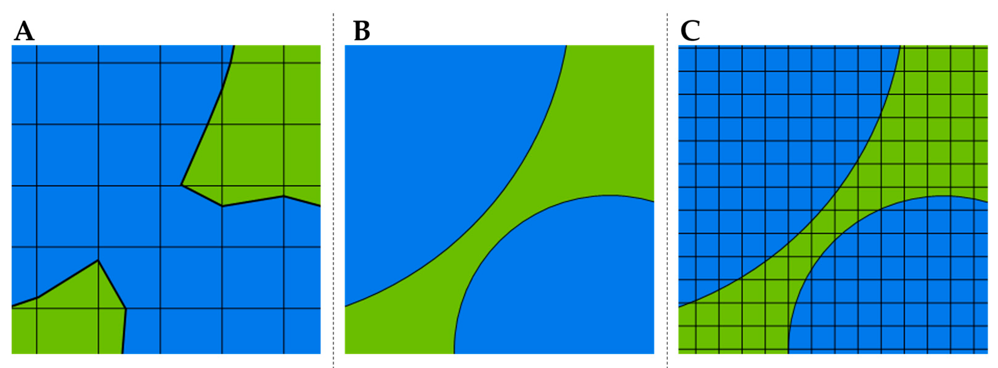
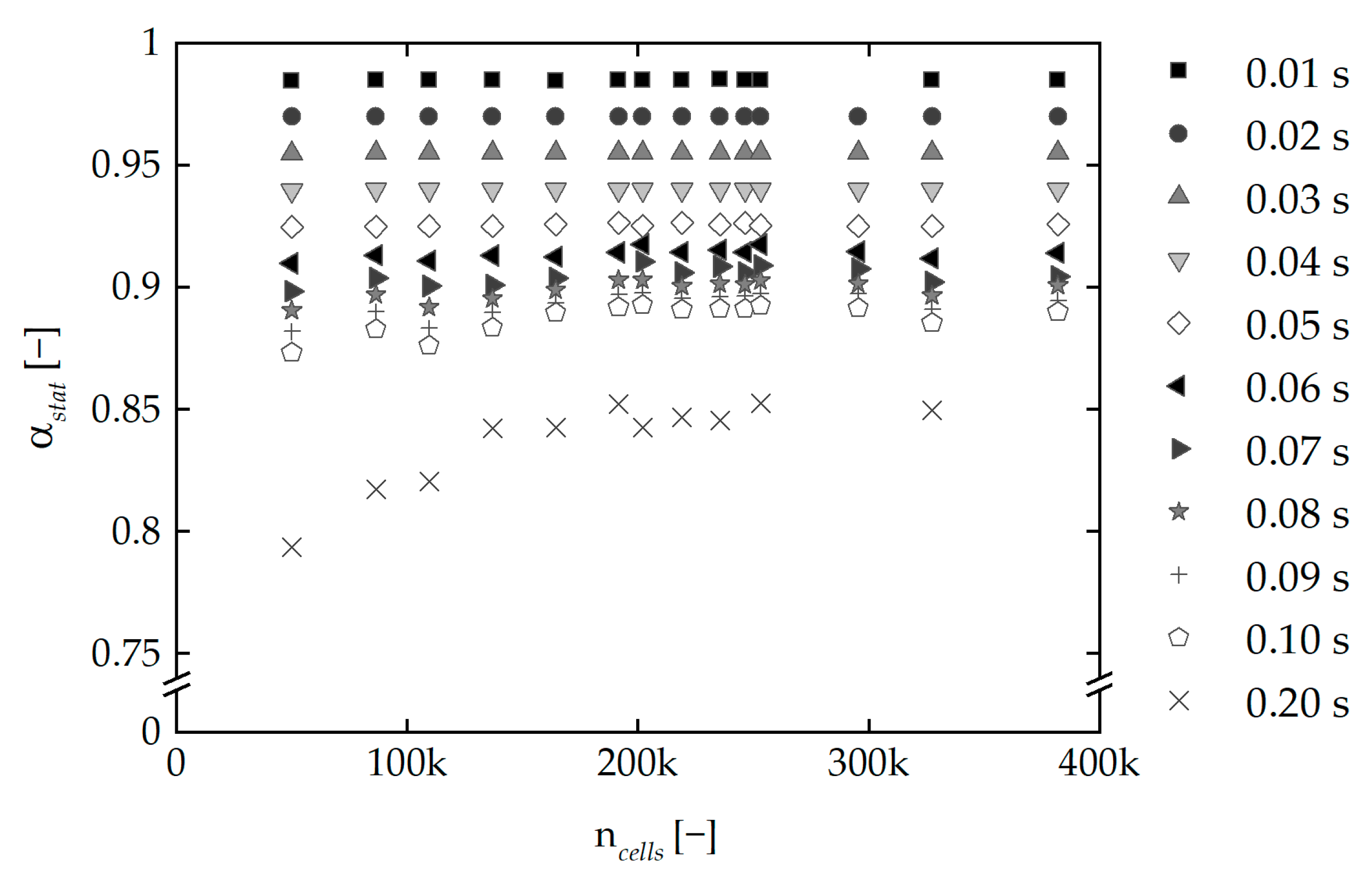
3.3. Mesh Independence Study

The mesh significantly influences the computational effort and the quality of a numerical simulation, whereby an optimum mesh size exists for each geometry. A mesh independence study determined this optimum for the two flow geometries shown in Figure A1. The maximum size of grid cells l m a x varied between 0.07 mm and 0.2 mm. Here, the mesh size of a selected computational mesh is reduced until a selected characteristic variable is constant. In this work, the quality of the meshes was determined by the phase fraction α averaged over the complete flow domain, as mentioned in Section 2.1. An overview of the grids investigated is shown in Table A1.
It must be considered that the phase fraction is time-dependent. The behavior of this variable was therefore studied at different timesteps. Figure 5 shows the results of the mesh independence study for a single-chamber flow area. It can be seen that α is only affected by the mesh size when simulating larger time spans (0.1 s and higher). Within those, α remains constant for a mesh of 191,555 CV and higher.
Here, the geometry is divided into 35 divisions in the z-direction and has a maximum mesh size of 0.1 mm. All the following simulations with a single-chamber flow area were therefore carried out with a mesh of 191,555 CV. The resulting mesh is presented in Figure A2. Generally, the phase fraction of the stationary phase α increases with increasing CV number. This is because the interface can be represented more clearly with the PLIC method as the mesh size decreases. The interface is less blurred with tight meshes, and detaching drops of the inflowing mobile phase can be represented more accurately than in coarse grids (Figure 3).
Despite the more accurate representation of the interphase when using finer meshes, it must be noted that modeling fine dispersions of the mobile phase in the chambers is visualizable to a limited extent when using the VoF method.

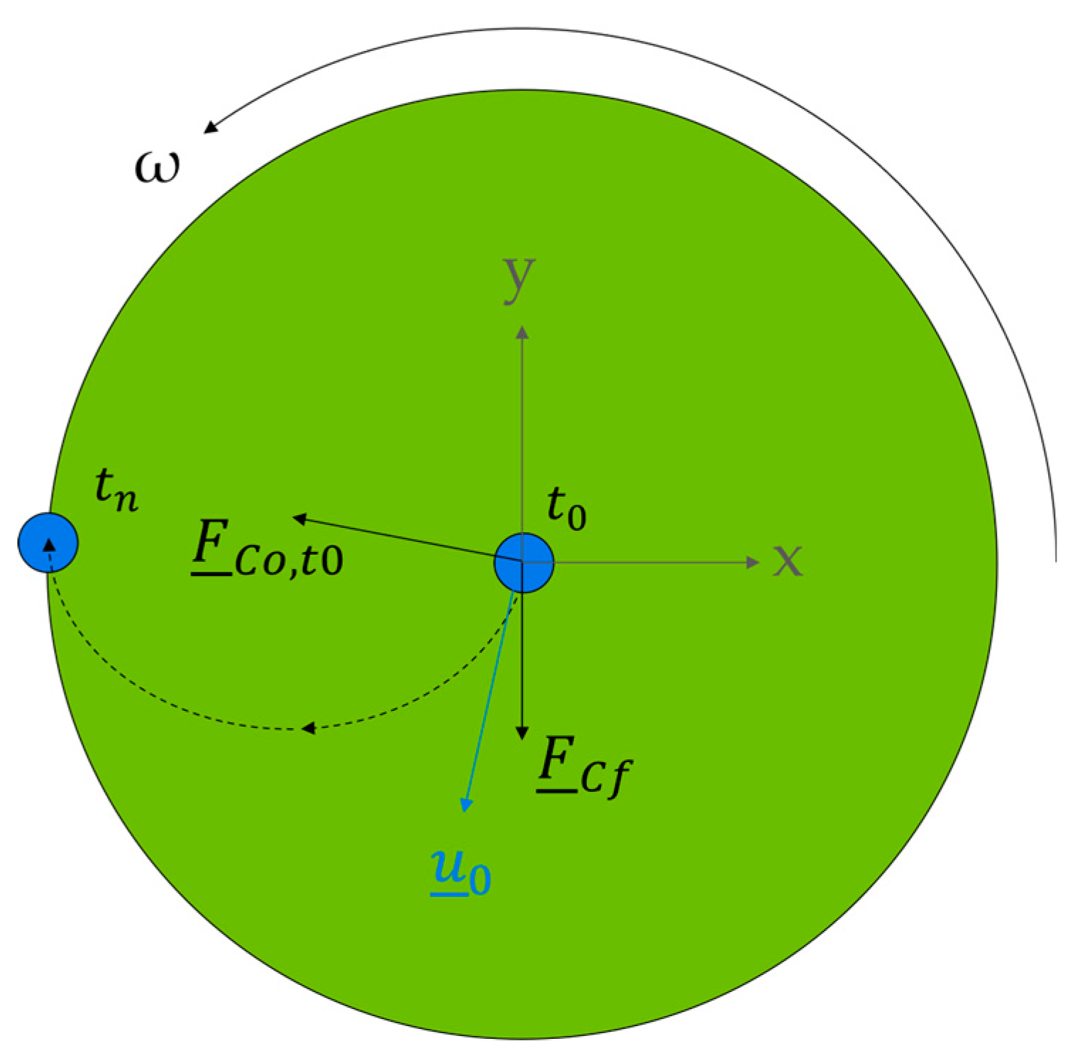
3.4. Rotational Forces in Single CPC Chambers

The effect of the rotational forces was investigated with the single-chamber flow area using the optimum mesh of 191,555 CV. Due to the centrifugal acceleration, a linearly increasing acceleration field is formed in the radial direction inside the CPC chambers. According to their different densities, the centrifugal force acts more firmly on the mobile than on the stationary phase. The centrifugal acceleration and the centrifugal force are shown in Figure A3. At a rotation of 1000 rpm and an inflow velocity of 0.15 m·s−1, the Coriolis acceleration is a hundred times smaller than the centrifugal acceleration inside the CPC rotor. This is because the Coriolis acceleration is—in contrast to centrifugal acceleration—independent of location. The force depends on the velocity only and is always orthogonal to it, resulting in a negligible small Coriolis force with decreasing inflow velocities. In contrast to the Coriolis force, the centrifugal force stays constant with changing fluid velocities. From the inlet to the outlet of the CPC chambers, the mobile phase is accelerated by centrifugal force. As an effect of that, the influence of the Coriolis force increases, and the mobile phase flows to the left wall.
Consequently, two vortices are formed in the chamber (Figure 6). The vortex in the upper part of the chamber rotates counterclockwise, and the vortex in the lower part rotates clockwise.

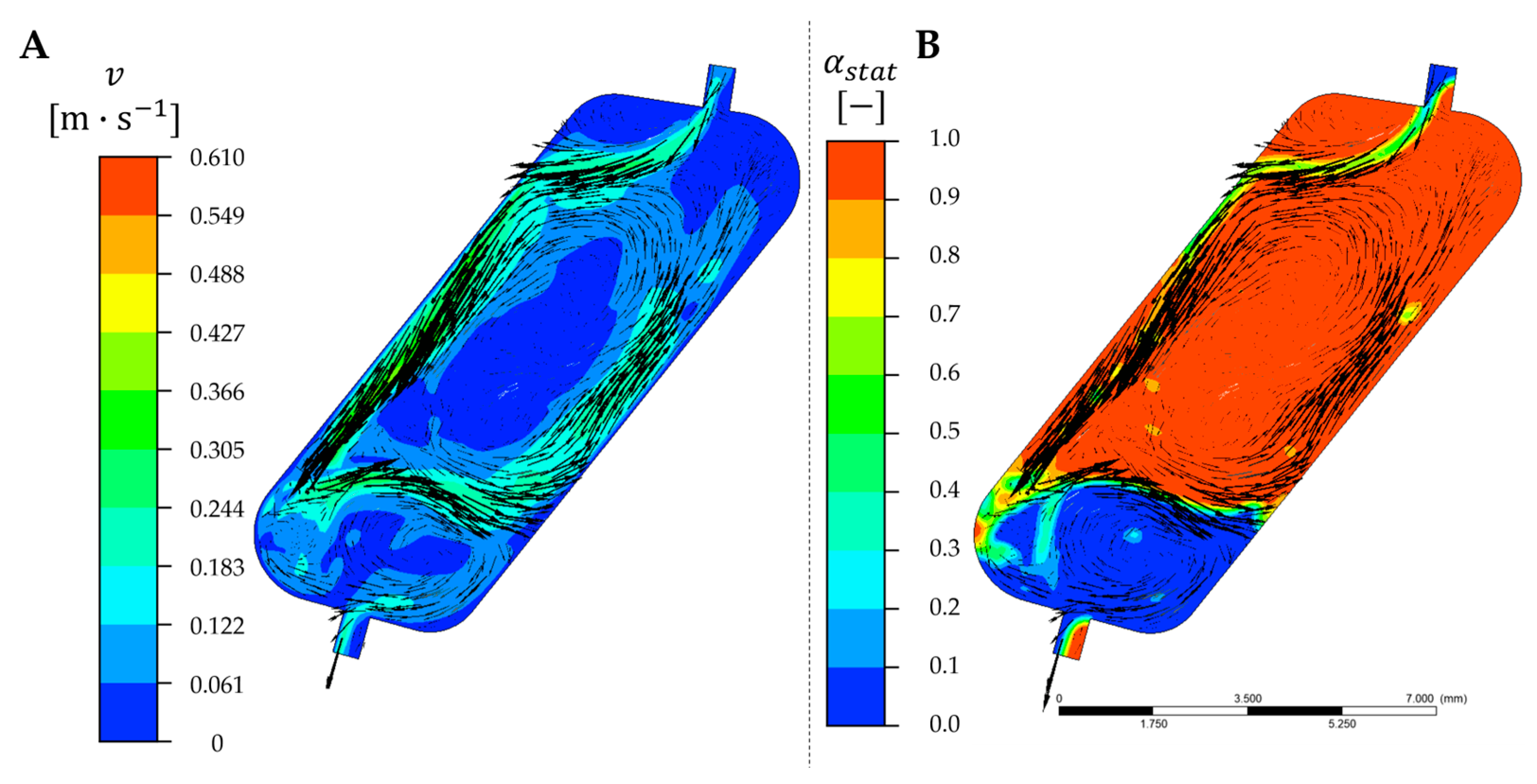
3.5. Velocity Field in Single CPC Chambers

An essential part of understanding hydrodynamics is investigating the velocity field inside the simulated CPC chambers. As part of the simulation, the velocity field of the entire flow area is determined using the conservation of momentum theorem at each time step. The resulting velocity field of the single-chamber flow area is shown in Figure 7A.
The velocity equals zero in the chambers’ upper left and right corners, representing dead zones. No convective transport occurs here, so the mass transfer is severely limited. The larger the dead zones, the poorer the separation performance of the CPC is. Experimental investigations have successfully optimized the chamber geometries toward minimizing the dead zones. However, the simulation indicates that completely avoiding dead zones is impossible due to adhesion effects at the chamber wall [24,42]. A maximal Reynolds number of 2250 was reached in the flow area (0.99 m·s−1), corresponding to laminar flow in accordance with the initial assumption (Section 2.1).
The distribution of the two phases and the velocity field were compared to estimate the effect of the volume and interfacial forces. Figure 7B shows the simulated chamber’s phase fraction and velocity field. One of the two vortices forms inside the dispersion zone, and the other vortex forms inside the coalescence zone. Several consistencies are evident when compared to experimental data (Figure 8). The inflowing mobile phase is deflected to the chamber wall, comparable to Figure 7B. The dead zones in the top edges and the middle of the chamber are of similar size, too. Moreover, the deflected boundary between the bulk phases has a comparable shape, indicating that the vortex formation is also present in the experimental setup.
The two swirls provide approximately ideal mixing within each phase. This is particularly important for the chromatographic separation performance of the CPC. Due to the increased surface area resulting from the dispersion of the mobile phase and the promoted mixing, both the surface and the volume-dependent mass transfer seem to occur under favorable conditions.

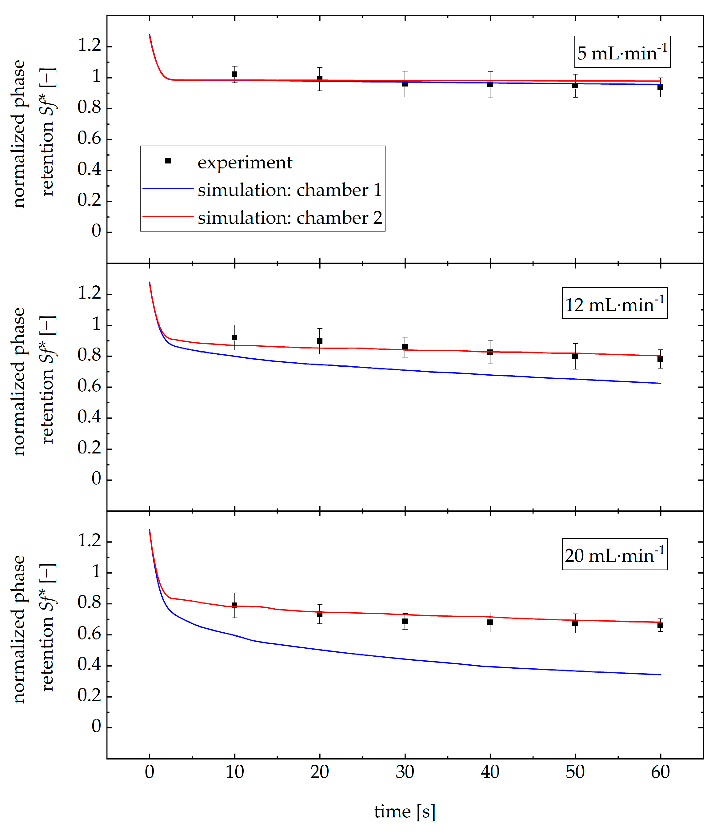
3.6. Comparison of Simulated and Experimental Retention Values in Single CPC Chambers

The retention of the chambers in the first viewing window of the rotor (chambers 4–7) was investigated experimentally to compare the experimental and simulation results. In contrast to the simulation results, where the volume fractions of the mobile and stationary phase are calculated during the process with the flowing mobile phase, the experimentally determined measurements were carried out with the pumps switched off. Only the resulting sharp linear phase boundary enables precise retention evaluation [40]. Raw data images recorded are shown in Figure A4. The images demonstrate that a part of the mobile phase is pushed back into the upstream channel when the pumps stop. Therefore, considering just the chambers, comparing the experimental and simulated results is insufficient.
As seen in Figure 9, experimental data indicate that the retention continuously falls during the observation time of 60 s. In the first 10 s, the decrease in the Sf* from 1.3 to 1.0 is most pronounced.
A comparison between the experimental and simulation results shows agreement regarding the general retention trend. However, there is a remarkable difference: while the experimental retention values fall over time, the simulated Sf* increases in the beginning before decreasing monotonously. Moreover, the simulated Sf* is lower than the experimental value in all cases. This is because of the backflow occurring at the chamber’s outlet. Here, the stationary phase reenters the flow area through the outlet. This is necessary for a valid simulation but contradicts the experimental observations, where this phenomenon did not occur. In addition, the simulated Sf* fluctuates over time. For validation of the simulation, it is essential to note that the simulation shows the first chamber of the rotor. However, the viewing window of the physical rotor does not allow for observation of the rotor’s first chamber. The first chamber visible in the video recordings is the fourth chamber of the rotor. The resulting uncertainty will be discussed in more detail when comparing the experimental and simulated data.

3.7. Simulation of Two Chambers

A second flow area was developed as an extension to the single-chamber-shaped one. The two-chamber flow area includes two chambers, the duct in between, and the duct at the outlet of the second chamber. In addition to that, it is possible to investigate the interaction of the individual chambers and the behavior of the flow inside the ducts. As mentioned, this flow area is shown in Figure A1. Analogously to the single-chamber flow area, a mesh independence study was carried out for the two-chamber flow area to find the optimal conditions for the simulation (Supplementary Information).
In the simulation of two linked chambers, the velocity profile differs slightly from that of a simulated single chamber. As in the single chamber, dead zones form in the upper right and left corners. A vortex formation in the upper and lower halves, along with the interface, is observable in both chambers. The maximum velocity in the second chamber is 1.1 m·s−1, which is higher than in the simulation of a single chamber (Section 3.5). The velocity field in the chambers and the direction of the flow are shown in Figure 10. As an example, for the entire flow area, the representation on a sectional plane in the middle x y-plane of the chambers is illustrated.
When comparing the simulated retention values in the two-chamber flow area with the experimental results gained, a significant improvement of congruence with the second (the left) chamber is noticeable (Figure 11). The latter is provided with a mixture of mobile and stationary phases withdrawn from the upstream chamber. Moreover, the simulated retention of the first chamber differs from the results shown in Figure 9. Because of the increased backpressure in the extended flow area, the backflow occurring at the flow area’s outlet is lower, directly impacting the retention value. Optimizing this “blurred” database would be possible with either an adapted rotor construction, where the first chamber is visible, or a simulation of even more chambers. However, the latter would drastically increase the computational effort and, therefore, is an undesirable option. To conclude, at least two cells should be simulated to create meaningful results in accordance with experimental observations, as discussed before.
Moreover, the volumetric flow rates of the mobile phase were altered: for 20 mL·min−1, the loss of the stationary phase over time is more pronounced. Nevertheless, the experimental results are comparable to the phase retention in the second chamber simulation, with the simulation of chamber 1 having comparatively low retention values. For 5 mL·min−1, the simulation results indicate a comparable behavior over time for both chambers. Again, the experimental results match the simulation.
When discussing these results in the context of experimental CPC runs (in the range of hours), the simulated bleeding rates in the first 60 s after startup and the bleeding rates after 60 min are comparable: In the case of 12 mL·min−1, the bleeding rate is 2.14·10−3 Sf*·s−1, compared to 3.06·10−3 Sf*·s−1 for the first chamber visible (chamber 4). For volumetric flow rates of 5 mL·min−1 (6.0·10−4 Sf*·s−1, compared to 7.03·10−4 Sf*·s−1) and 20 mL·min−1 (3.17·10−3 Sf*·s−1, compared to 5.24·10−3 Sf*·s−1), the same applies. These inaccuracies can be explained by the chamber offset, as mentioned above; the chamber analyzed is the fourth chamber of the rotor, whereas the simulated chamber is the second chamber. Therefore, more stationary phase of the upstream chambers is flushed into the chamber analyzed, increasing the bleeding rate compared to the simulation.

4. Conclusions

With the help of Computational Fluid Dynamics, we were able to simulate the retention characteristics of the phase system Arizona N in two chambers interconnected with ducts located in a higee environment. We determined the optimal mesh size using a mesh independence study. The stability of the flow fields was ensured by examining the phase fraction across different grid sizes and time steps. Therefore, we demonstrated that for our simulations, a dynamic equilibrium state was achieved by observing the constancy of the phase fraction with sufficiently small grid cells.
We measured and specified contact angles, contributing to the stability of boundary conditions in the simulation. In contrast to previous work, the simulation time was extended significantly using a high-performance computing cluster. Therefore, we were capable of modeling bleeding over increased periods of time for different volumetric flow rates, enhancing the understanding of hydrodynamics involved—not just during the startup of the apparatus (0.3 s of operation) but for a drastically prolonged time scale [28]. In conclusion, we took various measures regarding the stability of flow fields, the continuity of mass and momentum balance, the stability of boundary conditions, and the long-term stability to ensure a dynamic equilibrium state in our CFD simulations.
With a variation of input data, this model could be applied to different phase systems like aqueous two-phase systems or deep eutectic solvents, predicting the initial bleeding behavior. Nevertheless, the transfer of bleeding rates gained in the simulation to bleeding rates limiting the operation over long-time experiments should be validated in each case. In conclusion, simulation of systems’ stabilities in Centrifugal Partition Chromatography could be possible. After adaptation, even complex hydrodynamic phenomena like loss of stationary phase after sample injection could be addressed.
Detailed information about bleeding is necessary in order to predict bleeding in rotor setups with several hundred chambers. We will address this in upcoming research. Another thing to remember is that no retention data from the first chambers are available to date. That is why a second focus will be on rotor constructions not having that drawback.

Supplementary Materials

The following supporting information can be downloaded at https://www.mdpi.com/article/10.3390/separations11010016/s1, Figure S1: Mesh independence study for a two-chamber flow area; Table S1: Mesh independence study for a two-chamber flow area.

Author Contributions

Conceptualization, F.B., G.S. and J.K.; methodology, F.B.; software, S.V. and F.B.; validation, S.V. and F.B.; formal analysis, S.V. and F.B.; investigation, S.V. and F.B.; data curation, F.B.; writing—original draft preparation, F.B.; writing—review and editing, F.B., G.S. and J.K.; visualization, F.B.; supervision, G.S. and J.K. All authors have read and agreed to the published version of the manuscript.

Funding

This research received no external funding.

Data Availability Statement

Data is contained within the article or Supplementary Material.

Acknowledgments

The authors gratefully acknowledge the computing time provided on the Linux HPC cluster at Technical University Dortmund (LiDO3), partially funded in the course of the Large-Scale Equipment Initiative by the German Research Foundation (DFG) as project 271512359.

Conflicts of Interest

The authors declare no conflicts of interest.

Appendix A

Figure A1. (A) Flow area 1 of a single chamber. (B) Flow area 2 of two interconnected chambers with following channel.
Separations 11 00016 g0a1
Table A1. Overview of the variables altered in the mesh independence study for a single-chamber flow area.
l m a x
m m
n c e l l s , z
n c e l l s
10 4
l m a x
m m
n c e l l s , z
n c e l l s
10 4
l m a x
m m
n c e l l s , z
n c e l l s
10 4
0.1020110.0930200.20355
0.1025140.0830250.15359
0.1030160.0730330.093524
0.103519 0.083530
0.104022 0.073538
0.104525
Figure A2. Mesh for flow area 1 after mesh independence study with 191,555 CV.
Separations 11 00016 g0a2
Figure A3. Centrifugal acceleration and resulting centrifugal forces (arrows).
Separations 11 00016 g0a3
Figure A4. Exemplary raw data for determination of retention values. Mobile phase is dyed and appears dark grey.
Separations 11 00016 g0a4

References

  1. Chmiel, H. (Ed.) Bioprozesstechnik, 3rd ed.; Spektrum Akademischer Verlag: Heidelberg, Germany, 2011; ISBN 9783827424778. [Google Scholar]
  2. Schmidt-Traub, H.; Schulte, M.; Seidel-Morgenstern, A. (Eds.) Preparative Chromatography, 3rd ed.; Wiley-VCH: Weinheim, Germany, 2020; ISBN 978-3-527-34486-4. [Google Scholar]
  3. Foucault, A.P. (Ed.) Centrifugal Partition Chromatography; Dekker: New York, NY, USA, 1995; ISBN 9780824792572. [Google Scholar]
  4. Marchal, L.; Foucault, A.P.; Patissier, G.; Rosant, J.-M.; Legrand, J. Chapter 5 Centrifugal Partition Chromatography: An Engineering Approach. In Comprehensive Analytical Chemistry: Countercurrent Chromatography; Berthod, A., Ed.; Elsevier: Amsterdam, The Netherlands, 2002; pp. 115–157. ISBN 0166-526X. [Google Scholar]
  5. Kotland, A.; Chollet, S.; Diard, C.; Autret, J.-M.; Meucci, J.; Renault, J.-H.; Marchal, L. Industrial case study on alkaloids purification by pH-zone refining centrifugal partition chromatography. J. Chromatogr. A 2016, 1474, 59–70. [Google Scholar] [CrossRef]
  6. Berthod, A. (Ed.) Countercurrent Chromatography: The Support-Free Liquid Stationary Phase; Elsevier: Amsterdam, The Netherlands, 2002; ISBN 9780444507372. [Google Scholar]
  7. Friesen, J.B.; McAlpine, J.B.; Chen, S.-N.; Pauli, G.F. Countercurrent Separation of Natural Products: An Update. J. Nat. Prod. 2015, 78, 1765–1796. [Google Scholar] [CrossRef]
  8. Hopmann, E.; Arlt, W.; Minceva, M. Solvent system selection in counter-current chromatography using conductor-like screening model for real solvents. J. Chromatogr. A 2011, 1218, 242–250. [Google Scholar] [CrossRef]
  9. Frey, A.; Hopmann, E.; Minceva, M. Selection of Biphasic Liquid Systems in Liquid-Liquid Chromatography Using Predictive Thermodynamic Models. Chem. Eng. Technol. 2014, 37, 1663–1674. [Google Scholar] [CrossRef]
  10. Bezold, F.; Weinberger, M.E.; Minceva, M. Computational solvent system screening for the separation of tocopherols with centrifugal partition chromatography using deep eutectic solvent-based biphasic systems. J. Chromatogr. A 2017, 1491, 153–158. [Google Scholar] [CrossRef]
  11. Hopmann, E.; Frey, A.; Minceva, M. A priori selection of the mobile and stationary phase in centrifugal partition chromatography and counter-current chromatography. J. Chromatogr. A 2012, 1238, 68–76. [Google Scholar] [CrossRef]
  12. Krause, J.F. Biocatalytic Conversions in a Centrifugal Partition Chromatograph; Dr. Hut: München, Germany, 2017; ISBN 9783843934688. [Google Scholar]
  13. Almeida, M.R.; Ferreira, F.; Domingues, P.; Coutinho, J.A.P.; Freire, M.G. Towards the purification of IgY from egg yolk by centrifugal partition chromatography. Sep. Purif. Technol. 2022, 299, 121697. [Google Scholar] [CrossRef]
  14. Krause, J.; Oeldorf, T.; Schembecker, G.; Merz, J. Enzymatic hydrolysis in an aqueous organic two-phase system using centrifugal partition chromatography. J. Chromatogr. A 2015, 1391, 72–79. [Google Scholar] [CrossRef]
  15. Krause, J.; Merz, J. Comparison of enzymatic hydrolysis in a centrifugal partition chromatograph and stirred tank reactor. J. Chromatogr. A 2017, 1504, 64–70. [Google Scholar] [CrossRef]
  16. Berthod, A.; Ruiz-Ángel, M.J.; Carda-Broch, S. Recent advances on ionic liquid uses in separation techniques. J. Chromatogr. A 2018, 1559, 2–16. [Google Scholar] [CrossRef]
  17. Bezold, F.; Minceva, M. A water-free solvent system containing an L-menthol-based deep eutectic solvent for centrifugal partition chromatography applications. J. Chromatogr. A 2019, 1587, 166–171. [Google Scholar] [CrossRef]
  18. Bezold, F.; Roehrer, S.; Minceva, M. Ionic Liquids as Modifying Agents for Protein Separation in Centrifugal Partition Chromatography. Chem. Eng. Technol. 2019, 42, 474–482. [Google Scholar] [CrossRef]
  19. Bezold, F.; Goll, J.; Minceva, M. Study of the applicability of non-conventional aqueous two-phase systems in counter-current and centrifugal partition chromatography. J. Chromatogr. A 2015, 1388, 126–132. [Google Scholar] [CrossRef]
  20. Kopilovic, B.; Valente, A.I.; Ferreira, A.M.; Almeida, M.R.; Tavares, A.P.M.; Freire, M.G.; Coutinho, J.A.P. Towards the sustainable extraction and purification of non-animal proteins from biomass using alternative solvents. RSC Sustain. 2023, 1, 1314–1331. [Google Scholar] [CrossRef]
  21. Prinz, A. Enzyme Separation Using Aqueous Two-Phase Extraction: Experiment, Model and Simulation; Dr. Hut: München, Germany, 2014. [Google Scholar]
  22. van Buel, M.J.; van Halsema, F.E.D.; van der Wielen, L.A.M.; Luyben, K.C.A.M. Flow regimes in centrifugal partition chromatography. AICHE J. 1998, 44, 1356–1362. [Google Scholar] [CrossRef]
  23. Szekely, G.; Zhao, D. (Eds.) Sustainable Separation Engineering: Materials, Techniques and Process Development; John Wiley & Sons Ltd.: Hoboken, NJ, USA, 2022; ISBN 9781119740087. [Google Scholar]
  24. Schwienheer, C.; Merz, J.; Schembecker, G. Investigation, comparison and design of chambers used in centrifugal partition chromatography on the basis of flow pattern and separation experiments. J. Chromatogr. A 2015, 1390, 39–49. [Google Scholar] [CrossRef]
  25. Fromme, A.; Fischer, C.; Klump, D.; Schembecker, G. Correlating the phase settling behavior of aqueous-organic solvent systems in a centrifugal partition chromatograph. J. Chromatogr. A 2020, 1620, 461005. [Google Scholar] [CrossRef]
  26. Fromme, A.; Fischer, C.; Keine, K.; Schembecker, G. Characterization and correlation of mobile phase dispersion of aqueous-organic solvent systems in centrifugal partition chromatography. J. Chromatogr. A 2020, 1620, 460990. [Google Scholar] [CrossRef]
  27. Chollet, S.; Marchal, L.; Jérémy, M.; Renault, J.-H.; Legrand, J.; Foucault, A. Methodology for optimally sized centrifugal partition chromatography columns. J. Chromatogr. A 2015, 1388, 174–183. [Google Scholar] [CrossRef]
  28. Adelmann, S.; Schwienheer, C.; Schembecker, G. Multiphase flow modeling in centrifugal partition chromatography. J. Chromatogr. A 2011, 1218, 6092–6101. [Google Scholar] [CrossRef]
  29. Ansys®. Fluent; Ansys: Canonsburg, PA, USA, 2021. [Google Scholar]
  30. Cushman-Roisin, B. Introduction to Geophysical Fluid Dynamics: Physical and Numerical Aspects, 2nd ed.; Academic Press: Waltham, MA, USA, 2011; ISBN 9780080916781. [Google Scholar]
  31. Berthod, A.; Hassoun, M.; Ruiz-Angel, M.J. Alkane effect in the Arizona liquid systems used in countercurrent chromatography. Anal. Bioanal. Chem. 2005, 383, 327–340. [Google Scholar] [CrossRef]
  32. Vaessen, G. Predicting Catastrophic Phase Inversion in Emulsions. Ph.D. Thesis, Eindhoven University of Technology, Eindhoven, The Netherland, 1996. [Google Scholar]
  33. Paschedag, A. CFD in der Verfahrenstechnik: Allgemeine Grundlagen und mehrphasige Anwendungen; Wiley-VCH: Weinheim, Germany, 2005; ISBN 9783527603855. [Google Scholar]
  34. Schwarze, R. CFD-Modellierung: Grundlagen und Anwendungen bei Strömungsprozessen; Springer: Berlin/Heidelberg, Germany, 2012; ISBN 978-3-642-24378-3. [Google Scholar]
  35. Fromme, A. Systematic Approach Towards Solvent System Selection for Ideal Fluid Dynamics in Centrifugal Partition Chromatography; Dr. Hut: München, Germany, 2020; ISBN 9783843916110. [Google Scholar]
  36. Lomax, H.; Pulliam, T.H.; Zingg, D.W.; Kowalewski, T.A. Fundamentals of Computational Fluid Dynamics. Appl. Mech. Rev. 2002, 55, B61. [Google Scholar] [CrossRef]
  37. Fromme, A.; Funke, F.; Merz, J.; Schembecker, G. Correlating physical properties of aqueous-organic solvent systems and stationary phase retention in a centrifugal partition chromatograph in descending mode. J. Chromatogr. A 2020, 1615, 460742. [Google Scholar] [CrossRef]
  38. Adelmann, S.; Schembecker, G. Influence of physical properties and operating parameters on hydrodynamics in Centrifugal Partition Chromatography. J. Chromatogr. A 2011, 1218, 5401–5413. [Google Scholar] [CrossRef]
  39. Adelmann, S. On Hydrodynamics in Centrifugal Partition Chromatography; Dr. Hut: München, Germany, 2014; ISBN 9783843916110. [Google Scholar]
  40. Buthmann, F.; Pley, F.; Schembecker, G.; Koop, J. Automated Image Analysis for Retention Determination in Centrifugal Partition Chromatography. Separations 2022, 9, 358. [Google Scholar] [CrossRef]
  41. Ikehata, J.-I.; Shinomiya, K.; Kobayashi, K.; Ohshima, H.; Kitanaka, S.; Ito, Y. Effect of Coriolis force on counter-current chromatographic separation by centrifugal partition chromatography. J. Chromatogr. A 2004, 1025, 169–175. [Google Scholar] [CrossRef]
  42. Schwienheer, C. Advances in Centrifugal Purification Techniques for Separating (Bio-)chemical Compounds; Dr. Hut: München, Germany, 2016; ISBN 9783843929165. [Google Scholar]
Figure 1. Rotational forces acting on a fluid voxel (blue dot). The initial velocity u 0 , the centrifugal force F C f , and the Coriolis force F C o are shown. This results in a curved movement of the fluid to its position at a time step t n > t 0 .
Separations 11 00016 g001
Figure 2. (A) Modified FCPC rotor disk with 66 chambers and channels embedded. (B) Dimensions of a single chamber–channel combination [35].
Separations 11 00016 g002
Figure 3. A schematic course of the phase boundary using different computational meshes. (B) The actual course of the interface is shown. The interface calculated with a coarse mesh is presented on the left side (A), and on the right side, the interface is calculated with a fine mesh (C). Green/blue: different fluids.
Separations 11 00016 g003
Figure 4. Effect of rotational forces. A volume element (mobile phase) with a diameter of 10 mm is surrounded by the stationary phase. The total flow area is a 2D plate with a diameter of 100 mm. (B) At the time t 0 , the volume element moves with a velocity of 0.15 m·s−1 in the negative y-direction. (A) The left picture shows the simulated behavior of the volume element without rotation. (C) The right image shows a counterclockwise rotation of the flow area with 1000 rpm.
Separations 11 00016 g004
Figure 5. Results of the mesh independence study for a single-chamber flow area. The control variable α is stable from a maximum mesh size of 0.1 mm and 35 divisions in the z-direction. This corresponds to a mesh of 191,555 cells.
Separations 11 00016 g005
Figure 6. Coriolis acceleration in CPC chambers. The image shows the Coriolis acceleration and its direction in colored arrows and the velocity field direction in black arrows on a cross-sectional plane in the center of the chambers. The phase system used is Arizona N. The inlet velocity is 0.15 m·s−1, and the rotational speed is 1000 rpm counterclockwise. The picture shows the flow pattern after 10 s.
Separations 11 00016 g006
Figure 7. (A) Velocity field and its direction (black arrows) on a cross-sectional plane in the center of the chambers. (B) Phase fraction of the stationary phase in combination with the velocity field. The phase system used is Arizona N. The inlet velocity is 0.15 m·s−1, and the rotational speed is 1000 rpm counterclockwise. The pictures show the results after 10 s.
Separations 11 00016 g007
Figure 8. Experimental data of the first chamber visible (third chamber of the rotor). The mobile phase is dyed and, therefore, the darker fluid. The phase system used is Arizona N. The inlet velocity is 0.15 m·s−1, and the rotational speed is 1000 rpm counterclockwise. The picture was made after 10 s. Vortices are highlighted.
Separations 11 00016 g008
Figure 9. Comparison of the retention calculated in the simulation of a single chamber and the measured retention. The phase system is Arizona N. The time-dependent Sf* was recorded at a volume flow of 12 mL·min−1 and 1000 rpm counterclockwise.
Separations 11 00016 g009
Figure 10. Resulting velocity field for the simulation of two CPC chambers. The velocity is shown on the middle cross-sectional plane of the three-dimensional flow area. The direction of the velocity is marked with black arrows. The phase system used is Arizona N. The inlet velocity is 0.15 m·s−1, and the rotational speed is 1000 rpm counterclockwise. The picture was made after 10 s.
Separations 11 00016 g010
Figure 11. Comparison of the retention calculated in the simulation of two chambers and the measured retention for different volumetric flow rates. The phase system is Arizona N. The time-dependent Sf* was recorded at a volume flow of 5, 12, and 20 mL·min−1 and 1000 rpm counterclockwise.
Separations 11 00016 g011
Table 1. Physical properties (at 25 °C) of the Arizona N system used [37].
Phase ρ
k g · m 3
η
m P a s
γ
m N · m 1
organic phase748.4 ± 2.20.3755 ± 0.00172.9717 ± 0.1776
aqueous phase928.1 ± 10.81.4632 ± 0.0047
Table 2. Contact angle measurement results with Arizona N at room temperature.
Fluid 1Fluid 2Solid θ   ° T   ° C
upper phasesaturated vaporstainless steel < 10 26.4   ±   0.0
lower phasesaturated vaporstainless steel 34.7   ±   3.3 26.8   ±   0.0
upper phasesaturated vaporseal (FEP) 28.2   ±   1.7 27.1   ±   0.1
lower phasesaturated vaporseal (FEP) 59.5   ±   2.8 26.9   ±   0.0
lower phaseupper phasestainless steel 121.9   ±   5.7 26.2   ±   0.1
lower phaseupper phaseseal (FEP) 127.8   ±   3.4 26.6   ±   0.0
Disclaimer/Publisher’s Note: The statements, opinions and data contained in all publications are solely those of the individual author(s) and contributor(s) and not of MDPI and/or the editor(s). MDPI and/or the editor(s) disclaim responsibility for any injury to people or property resulting from any ideas, methods, instructions or products referred to in the content.

