Article

CFD Simulation and Optimal Design of a New Parabolic–Shaped Guided Valve Tray

School of Chemical Engineering, East China University of Science and Technology, Shanghai 200237, China
*
Author to whom correspondence should be addressed.
Separations 2023, 10(4), 267; https://doi.org/10.3390/separations10040267
Submission received: 24 February 2023 / Revised: 26 March 2023 / Accepted: 17 April 2023 / Published: 20 April 2023
(This article belongs to the Special Issue Advances in Separation Engineering)

Abstract

:
A new parabolic–shaped guided valve tray is proposed. The gas–liquid two–phase flow of parabolic and conventional rectangular guided valve trays is simulated using the computational fluid dynamics (CFD) method. The clear liquid height on the tray was predicted for different combinations of the superficial gas velocity, liquid flow intensity and weir height. The predicted values were in good agreement with the calculated ones. The parabolic–shaped guided valve tray has a more uniform flow form by comparing the gas–liquid two–phase flow behavior of parabolic and rectangular guided valve trays: the liquid level difference is slight, the guiding effect is strong, and the re–mixing phenomenon is improved. Further modeling and simulations were conducted for nine parabolic–shaped guided valve trays of different function expressions. The optimum valve structure is the parabolic–shaped guided valve of the a–value at 0.075 and the t–value at 26.

1. Introduction

Distillation columns are essential equipment to separate liquid mixtures widely used in chemical, petroleum, pharmaceutical, and environmental industries [1,2,3,4]. The performance of the valve tray can directly affect the raw material handling capacity and product quality. The rectangular guided valve tray has high flux and mass transfer efficiency compared to the sieve and fixed valve trays, which are widely used in the practical industry [5,6,7,8]. However, with the increasing industrial demand, the shortcomings of the traditional guided valve have gradually emerged. The gas enters the valve tray along both sides of the valve bore perpendicular to the valve cover, which has a weak guiding effect. The airflow between the valves forms a vortex, leading to the return of liquid mixing. Valve legs at the front and rear end of the valve body impede the gas flow, and the liquid is deposited in this area, forming a dead flow zone. Therefore, there is an urgent need for a better–performing valve tray structure to complete the separation task. This paper proposes a new parabolic–shaped guided valve tray. A comparative study of the specific gas–liquid two–phase flow patterns of parabolic and rectangular guided valves is required to verify their hydrodynamic performance under certain operating conditions.
In recent years, computational fluid dynamics (CFD) has become a powerful tool for analyzing gas–liquid two–phase flow on a valve tray. Compared with experimental methods, CFD is highly flexible and can quickly change the valve tray’s structural dimensions and operating conditions to predict the fluid flow process in more detail, saving time and economic costs [9,10,11,12]. Many researchers have successively simulated and calculated the flow characteristics of trays such as sieve trays, guided valves, and fixed valves, comparing them with experiments to verify the reliability of the CFD simulation results. Liu et al. [13] and Yu et al. [14] simulated two–dimensional two–phase flow on conventional sieve trays, ignoring the effect of the variation of the gas phase along the height direction of the tray. Fischer and Quarini simulated three–dimensional transient two–phase flow on trays, assuming a traction coefficient of a constant 0.44, which only applies to homogeneous bubble flows and not to the flow behavior in the foam or spray regimes [15,16]. Krishna et al. estimated a new correlation equation for the traction coefficient, which applies to bubble populations [17,18]. Their work provides theoretical guidance for studying complex gas–liquid two–phase flows on trays and provides a solid basis for designing and optimizing them.
In this paper, three–dimensional transient CFD models were developed for the rectangular guided valve and parabolic–shaped guided valve trays. The correlation equation for the mean gas phase fraction was loaded into Fluent fitted by Yufeng Ma et al. via a user–defined function (UDF) [6]. Simulations were carried out under various combinations of weir height, gas, and liquid flow rates compared with the correlation equation to verify the correctness of the proposed model. The hydrodynamic performance of the rectangular guided valve and parabolic–shaped guided valve tray were compared based on the simulation results. Moreover, the characteristics of the phase fraction distribution, two–phase flow velocity distribution, and clear liquid height were investigated for both. The optimal parabolic–shaped valve structure is further modeled and simulated for the parabolic–shaped guided valve tray of nine different function expressions by comparing the mean liquid phase velocity along the direction of flow of the main body at different tray heights.

2. CFD Model

2.1. Control Equations

The column structure, feed conditions, and operating parameters influence the gas–liquid two–phase flow in the column space, resulting in an unfavorable back–mixing phenomenon and a highly complex flow state. The Eulerian model assumes that the two turbulent fluids co–exist in time. Both phases are considered interpenetrating continua with independent transport equations, whose laws of motion follow their respective governing differential equations. The Eulerian model is used as it provides a more accurate description of the interaction between the two phases and is consistent with the actual flow conditions of the gas and liquid phases on the tray. Where the gas and liquid phases are considered as the dispersed and continuous phases, respectively, the control equations are as follows [19,20,21]:
Continuity Equations:
α G ρ G t + α G ρ G u G = 0
α L ρ L t + α L ρ L u L = 0
Momentum Equations:
t α G ρ G u G + α G ρ G u G u G = α G μ G u G + u G T α G p G + α G ρ G g + M G L
t α L ρ L u L + α L ρ L u L u L = α L μ L u L + u L T α L p L + α L ρ L g M L G
where ρ, u, α, μ represent the macroscopic density, velocity, volume fraction, and viscosity, respectively, p is the pressure, and g is the gravitational force. The subscripts G and L represent the gas and liquid phases, respectively. Simultaneously, the same pressure field has been assumed for both phases:
p G = p L
The gas and liquid volume fractions, αL and αG are related by the summation constraint:
α G + α L = 1
MGL represents the source term of momentum transfer between two phases of gas and liquid, describing the inter–phase momentum exchange process caused by the inter–phase forces. The interphase forces are equal in magnitude and opposite in direction, with a combined force of zero:
M G L = M L G

2.2. Closure Conditions

For gas–liquid two–phase flow on a tray, the source terms for momentum transfer between phases include drag force, virtual mass force, and lift force. Krishna and Baten proposed that virtual mass force and lift force have limited effects on bubble flow and can be neglected compared to traction force [17,18]. Using the gas phase as the dispersed phase, the equation for MGL:
M G L = 3 4 C D d G α G ρ L u G u L u G u L
where CD is the dimensionless drag coefficient, and dG is the bubble diameter. Krishna et al. proposed a drag model applicable to bubble populations with the following expression for the drag coefficient [22]:
C D = 4 3 ρ L ρ G ρ L g d G 1 V 2 s l i p
where Vslip is the slip velocity of the bubble swarm with respect to the liquid, which can be estimated from superficial gas velocity Us and the average gas hold–up fraction α G a v e r a g e :
V s l i p = U S α G a v e r a g e
Substituting the expressions for CD and Vslip into the equations for MGL and considering the effect of the liquid phase fraction, the resistance expression is modified to the following form:
M G L = α G α L g ρ L ρ G α G a v e r a g e 2 1 α G a v e r a g e U S 2 u G u L u G u L
The above equation does not need to consider the effect of bubble diameter on the drag force, which can improve the accuracy of the calculation. The mean gas phase fraction α G a v e r a g e is the key to solving the momentum source term MGL. For different trays, this corresponds to different average gas phase fractions α G a v e r a g e . Based on the equation for sieve trays established by Bennett [23] and combined with experimental data, Yufeng Ma et al. fitted the correlation equation for the mean gas phase fraction of rectangular guided valve trays [6]:
α G a v e r a g e = 1 exp 21.542 U S ρ G ρ L ρ G 1.0687
This paper uses the above correlations to simulate a rectangular guided valve tray and a parabolic–shaped guided valve tray, with the momentum source term coded into a user–defined function to calculate the solution.
The standard kε model is currently the most widely used turbulence model and has been applied to CFD simulations of trays in much of the literature [24,25,26]. In this paper, the standard kε model is used to provide closure of the Eulerian two–phase flow model with the mathematical expression [27,28]:
ρ k t + ρ k u i x i = x i μ + μ t σ k k x j + G k ρ ε
ρ ε t + ρ ε u i x i = x j μ + μ t σ ε ε x j + C 1 ε ε k G k C 2 ε ρ ε 2 k
Gk is the term for generating the rheostatic energy k due to the mean velocity gradient and is calculated by the following equation:
G k = μ t u i x j + u j x i u i x j
The model constants take the following values:
C = 1.44, C = 1.92, Cμ = 0.09, σk = 1.0, σε = 1.3.

2.3. Geometric Model of the Tray with Boundary Conditions

The geometric models of the rectangular guided valve tray and the parabolic–shaped guided valve tray are shown in Figure 1, and the individual valve structures are shown in Figure 2. In order to verify that the parabolic–shaped guided valve has an advantage over the rectangular guided valve, all other structural parameters are considered the same except for the different shapes of the valves. The tray diameter is 1200 mm, the weir length is 800 mm, the weir height is 54 mm, the bottom gap is 15 mm, the tray spacing is 450 mm, and the opening rate is 9.6%. The maximum opening of the valve is 15 mm, the guide hole height is 5 mm, the rectangular valve is 70×25 mm, the valve cover is 78×31 mm, the parabolic–shaped valve has a bottom edge length of 37/10 mm and a height of 63 mm, and the valve cover has a bottom edge length of 43/16 mm and a height of 71 mm. In order to save calculation time and computer memory, only half of the tray is taken for simulation due to its symmetry.
The liquid enters the mass transfer zone of the valve tray from the bottom gap of the downcomer and turns over the overflow weir to reach the bottom of the downcomer. In order to ensure that the downcomer leaves a certain liquid layer height, the bottom is equipped with a liquid seal tray, and finally, the liquid flows out from the liquid seal tray. The gas enters the tray space from both sides of the valve and the guide hole. Then flows out from the valve hole of the upper layer of the valve tray.

2.4. Meshing and Solution Algorithms

The entire calculation domain is meshed using a mixed structural and non–structural meshing method. The valve structure is more complex near the wall of the tray and is encrypted. The higher the number of meshes, the higher the accuracy of the calculation, but this requires a considerable amount of computer performance. The final choice of grid number 1,972,192 was made, with an 8 mm unstructured tetrahedral mesh at the bottom and top of the tray and an 8 mm structured hexahedral mesh in the remaining area. The meshing of the tray space is shown in Figure 3.
CFD solver setup: This paper uses the air–water system to simulate the gas–liquid two–phase flow field on the tray under two kinds of valve fully open conditions. Simulated working parameters: liquid flow intensity QL/Lw =20 m3/(m·h), valve hole kinetic energy factor F0 = 7.53 (m/s) (kg/m3)0.5, weir height hw = 0.054 m. Fluent’s software completed the simulation process using a non–constant implicit solver with a time step of 0.002 s, a first–order windward format for the discretization method, and the Phase Coupled SIMPLE method for the pressure–velocity coupling equation, with a calculation accuracy of 10−3. In addition, in order to speed up convergence and save calculation time, before the start of the calculation, the volume fraction of the gas phase in the flow region was initialized before the calculation started. The gas phase fraction of 0–170 mm on the tray was set to 50%, the gas phase fraction of −450 to −350 mm in the downcomer region was set to 0, and the remainder of the tray was set to 100% gas phase. The clear liquid height on the tray in the calculation area was also monitored transiently as a criterion to determine whether the gas–liquid phase flow had reached dynamic equilibrium.

3. Results and Discussion

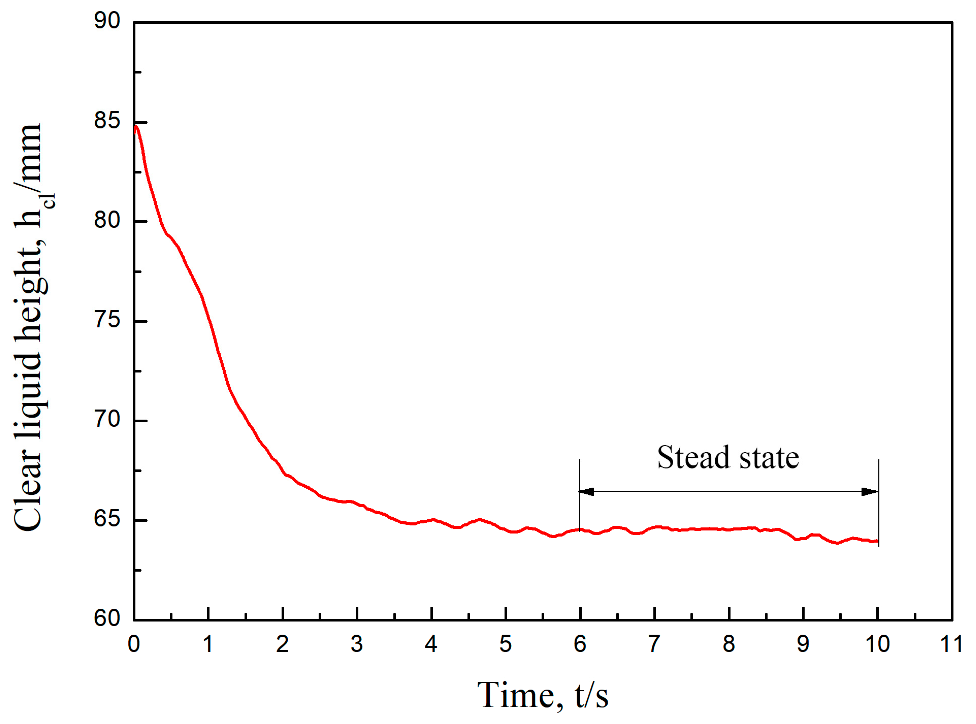
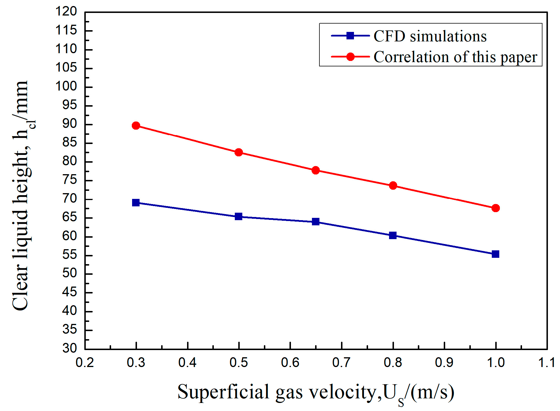
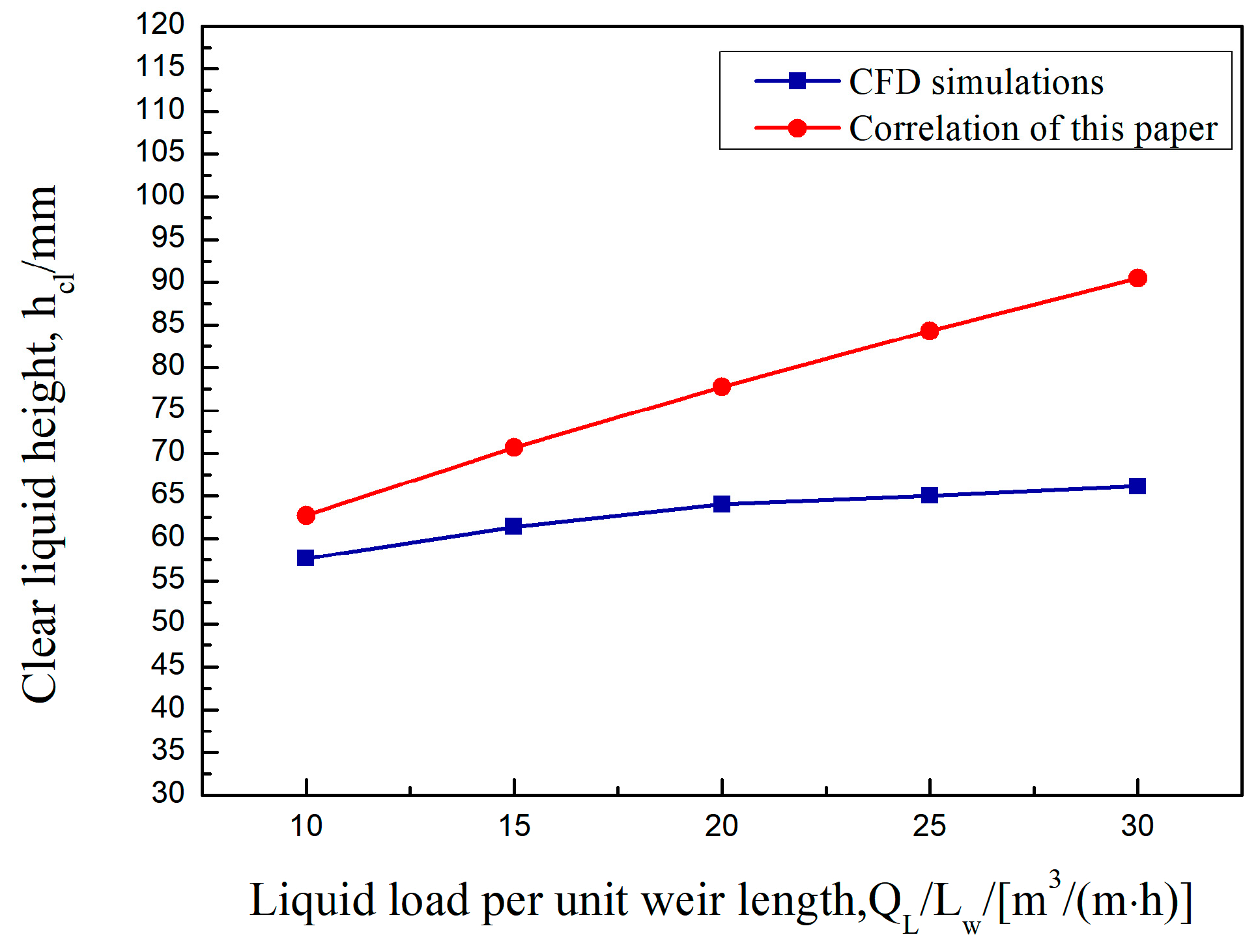
3.1. Model Validation

This paper uses the mean gas phase fraction correlation equation for a rectangular guided valve tray to simulate the proposed parabolic–shaped guided valve tray. The transient simulation is considered to have reached convergence when the height of the clear liquid height does not change significantly with time. As shown in Figure 4, after the start of the simulation, there is no more significant change in the clear liquid height around 6 s, indicating that the calculation has converged.
For valve trays, the clear liquid height is mainly influenced by the superficial gas velocity US, the liquid flow intensity QL/Lw, and the weir height hW. The correlation between the clear liquid height takes the following form [6]:
h c l = α L a v e r a g e h w + C Q L α L a v e r a g e 2 3
C = 1.475 + 1.385 exp 216 h w
In this paper, the values of clear liquid height obtained by CFD simulation under the same operating conditions are compared with the calculated values of the fitted formula. As shown in Figure 5, Figure 6 and Figure 7, the clear liquid height is positively correlated with the superficial gas velocity and negatively correlated with the liquid flow intensity and weir height. The difference between the simulated and calculated values is slight. The trend is consistent, indicating that the average gas phase fraction correlation of the rectangular guided valve applies to the modified parabolic–shaped guided valve, thus verifying the correctness of the CFD model developed.

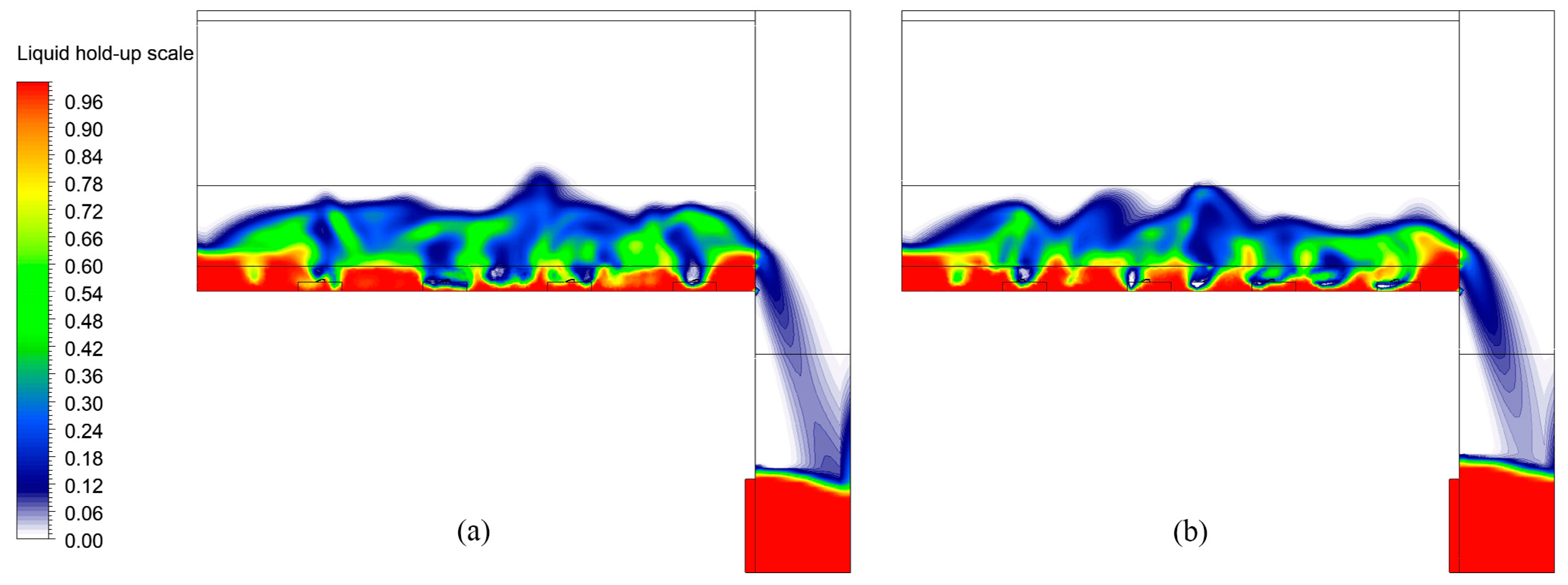
3.2. Gas–Liquid Phase Fraction Distribution

3.2.1. Liquid Phase Fraction Distribution

After the convergence of the simulations, the liquid phase fraction distribution in the xy section at z = −27.5 mm for the rectangular guided valve and parabolic–shaped guided valve tray is shown in Figure 8. As can be seen from the figure, the liquid phase fraction distribution at the bottom of the parabolic–shaped guided valve tray is more uniform and has a better flow pattern.

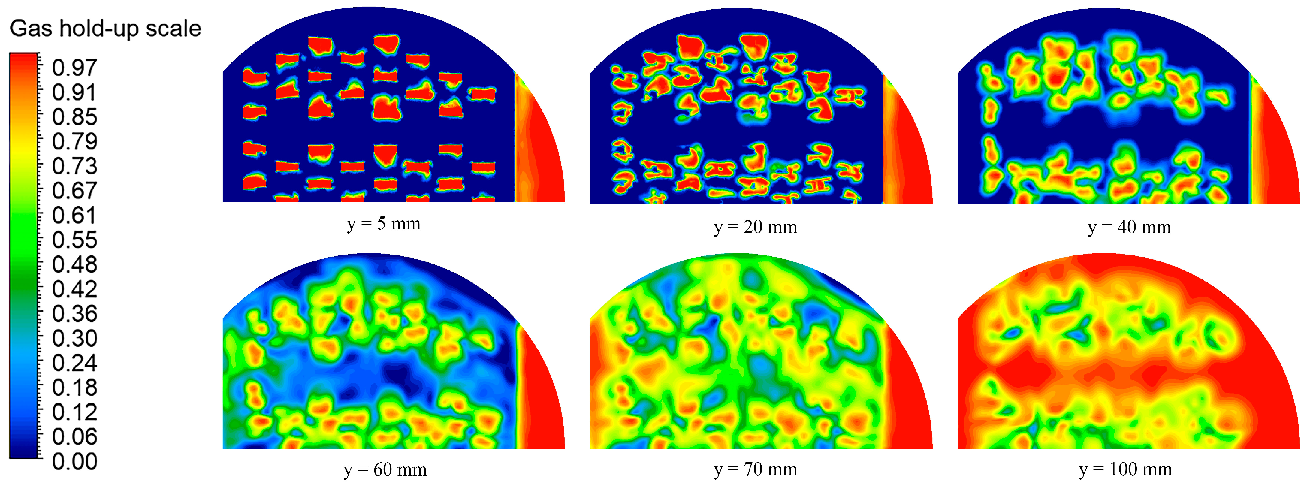
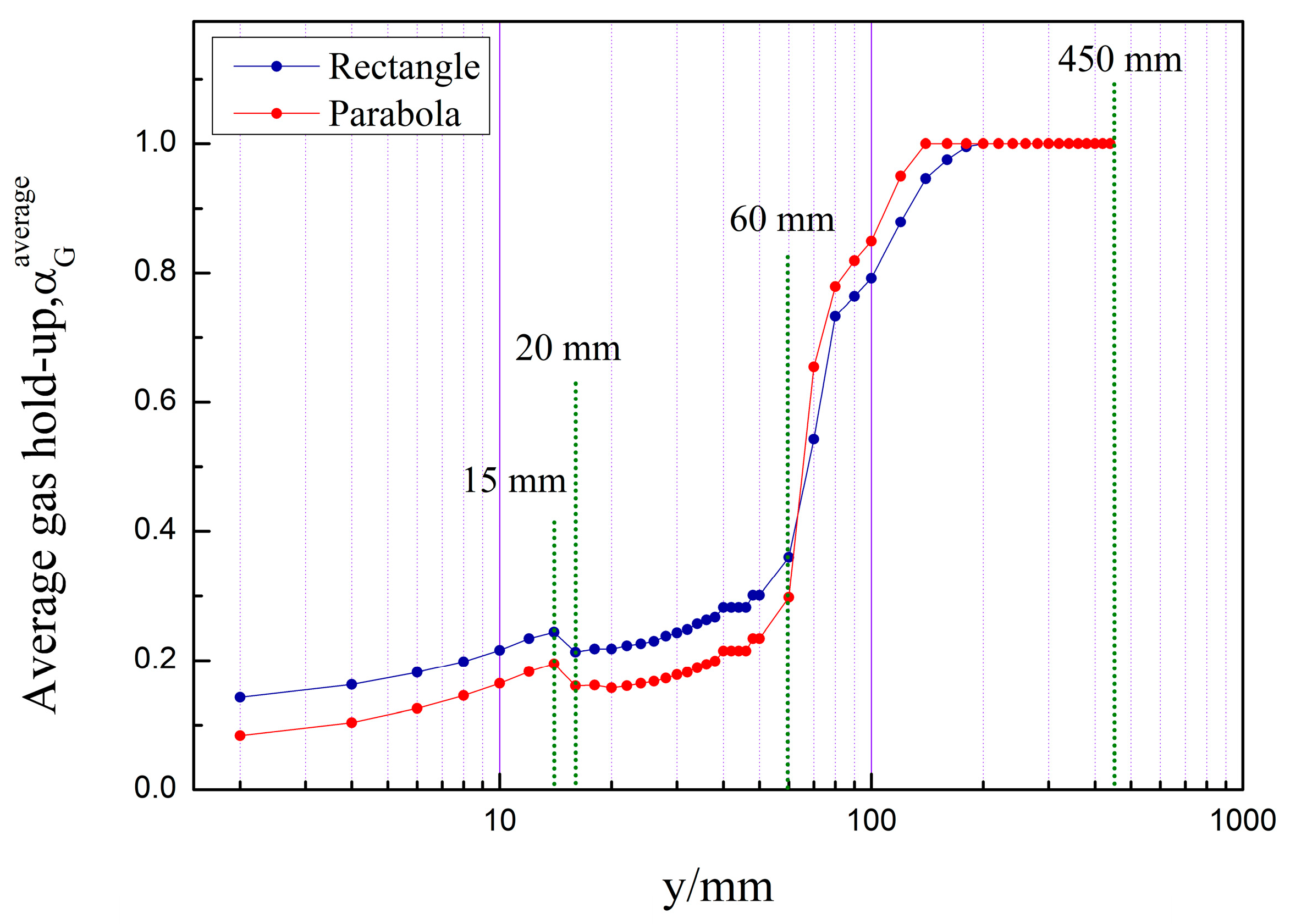
3.2.2. Gas Phase Fraction Distribution

The distributions of the gas phase fraction at different heights of the two valve trays are shown in Figure 9 and Figure 10. As seen from the figures, the gas phase fraction of the two valve trays generally follows the same trend with height. At y = 20 mm, the gas phase fraction decreases significantly, indicating that there will be a blind flow area above the valve cover. As the height gradually increases, the gas phase is dispersed, the gas phase fraction at a single point decreases, and the gas phase fraction at the same height tends to be uniform. After crossing the transition zone, the gas phase fraction increases sharply. The parabolic–shaped guided valve has a more uniform distribution of the gas phase fraction at the same height in the transition zone than the rectangular guided valve. In the gas phase continuity zone, the gas phase fraction is higher in the parabolic–shaped guided valve tray, indicating an improvement in mist entrainment.
A visual representation of the monotonicity variation is shown in Figure 11. As seen from the figure, the variation of the gas phase fraction of the two valve trays is not monotonically increasing with height. At y = 0–15 mm, the gas phase fraction increases monotonically with height. At y = 15−20 mm, the gas phase fraction decreases monotonically with height. At y > 20 mm, the gas phase fraction increases monotonically with height. At 0–60 mm, the gas phase fraction of the parabolic–shaped guided valve tray is lower than that of the rectangular guided valve tray. While at y > 60 mm, the gas phase fraction of the parabolic–shaped guided valve tray is higher than that of the rectangular guided valve tray. It indicates that the liquid phase continuous zone and the gas phase continuous zone of the parabolic–shaped guided valve are more distinct than the rectangular guided valve tray.

3.2.3. Variation of Clear Liquid Height along the x–Axis

Figure 12 shows the simulation results for the clear liquid height in the x–direction. After the convergence of the simulation, the typical cross–section in the direction of liquid flow is taken at equal intervals. Each cross–section’s average liquid phase fraction is calculated and multiplied by the tray spacing to obtain the clear liquid height. As seen from the graph, the clear liquid height shows periodic fluctuations, with the trough appearing at the opening of the valve, and the number of troughs is consistent with the number of valve columns. At this time, a large amount of gas is ejected from around the valve and the pilot hole, pushing the liquid forward, and the liquid layer at the pilot hole drops sharply, and a trough appears. The parabolic–shaped guided valve tray has a minor liquid level difference, unlike the rectangular guided valve tray. The level at each wave peak and trough is essentially the same, indicating that the parabolic–shaped guided valve tray has a more uniform flow pattern.

3.2.4. Variation of Clear Liquid Height along the z–Axis

As Figure 13 represents the simulation results of the clear liquid height along the z–direction, the clear liquid height is calculated similarly to the x–direction described before. As can be seen from the figure, the clear liquid height shows large fluctuations in the z–direction. The gas–liquid interaction is significant in the valve arrangement area, and the clear liquid height is low. The valves are sparsely arranged with significant gaps in the area between the bow tray and the channel tray, and the clear liquid height is high. Near the tower wall, the number of valves is small, the liquid phase flow rate is low, and the clear liquid height is high. The clear liquid height at the wave’s crest is lower in the parabolic–shaped guided valve tray than the rectangular guided valve tray, indicating that the parabolic–shaped guided valve tray has a more uniform flow pattern.

3.3. Gas–Liquid Phase Velocity Distribution

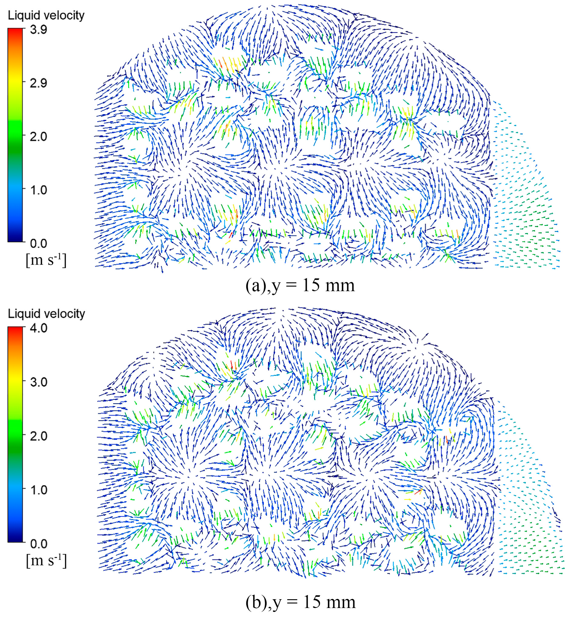
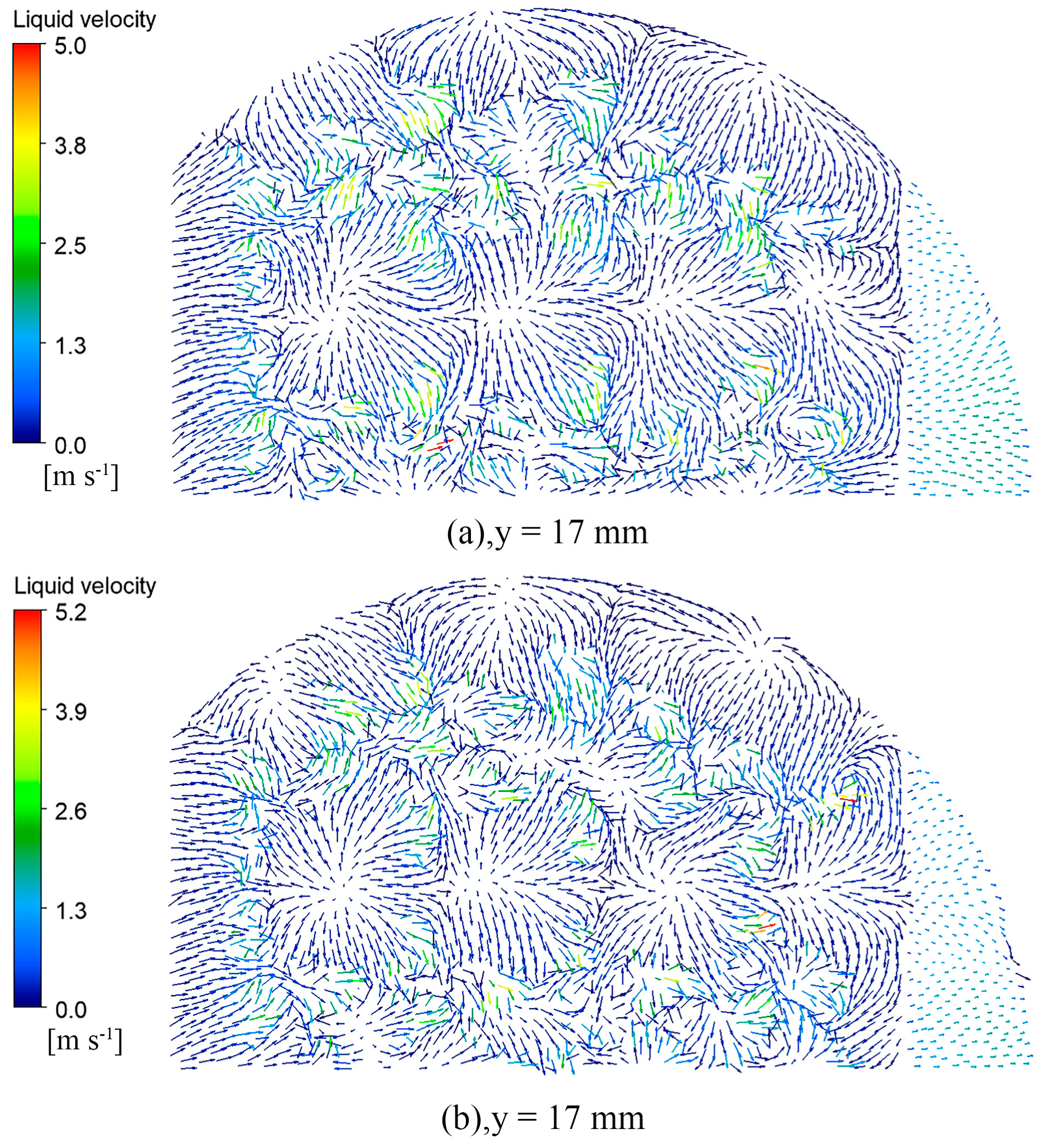
3.3.1. Liquid Phase Velocity Distribution

Figure 14, Figure 15, Figure 16 and Figure 17 show the vector diagram of the liquid phase velocity distribution at different heights on the two valve trays after the simulation convergence. In the region below the valve cover, at y < 15 mm, the gas is ejected from the valve hole at high speed, violent momentum transfer occurs with the liquid, and the liquid velocity of the parabolic–shaped guided valve tray can be increased from the initial 0.37 m/s to 8.2 m/s. The liquid velocity in the dense region of the valve is significantly higher than that in the sparse region. From the velocity vector diagrams of the liquid phase at y = 15 mm and y = 17 mm, it can be observed that there is a clear velocity component along the x–direction at the y = 17 mm pilot hole, which drives the liquid layer towards the outlet weir. The turbulence of the gas–liquid phase at the pilot hole is not as intense as in the area below the bonnet but still has a sizeable liquid velocity compared to the area above the pilot hole at y = 30 mm.
As can be seen from the diagram, the parabolic–shaped guided valve tray has a more incredible liquid velocity compared to the rectangular guided valve tray. The gas is ejected along the edge of the valve cover, and the velocity component increases in the x–direction, further reducing the liquid surface gradient. The parabolic–shaped guided valve has a velocity component along both sides and in front of the slope, which results in finer and more homogeneous gas dispersion, reduces the dead zone at the front of the valve, increases gas–liquid contact, and enhances inter–phase mass transfer. The simulation results confirm that the parabolic floating valve has a more substantial guiding effect and less dead space.

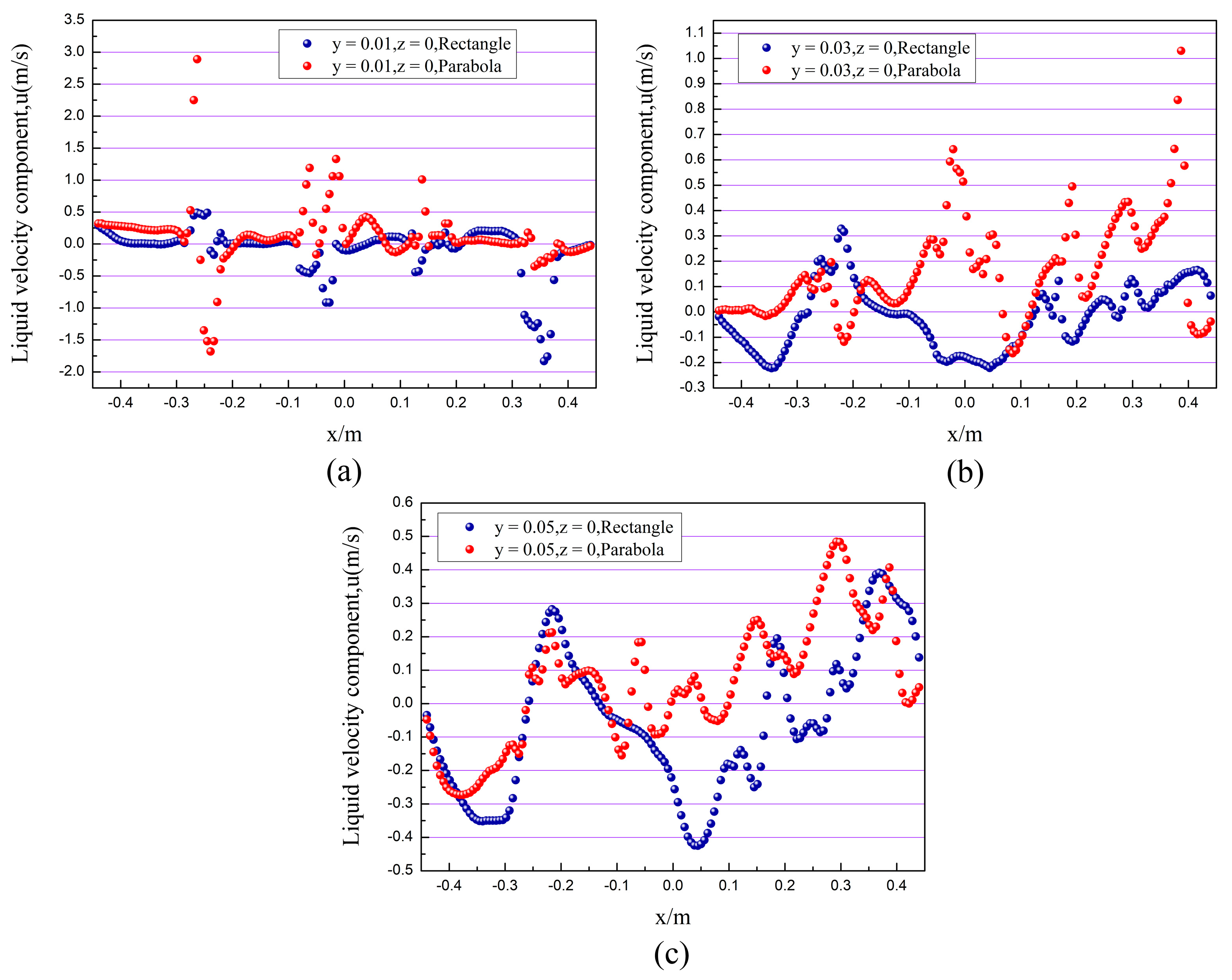
3.3.2. Velocity Distribution of the Liquid Phase in the x–Direction

Figure 18 shows the velocity distribution of the liquid phase in the x–direction corresponding to different heights at z = 0, calculated for the simulation conditions of US = 0.65 m/s, QL/LW = 20 m3/(m·h) and hW = 0.054 m. As can be seen from the graph, the component of the flow velocity in the x–direction near the liquid phase inlet above the valve cover is harmful, with a significant backflow phenomenon, and it increases with height. The parabolic–shaped guided valve tray has a higher liquid phase velocity in the x–positive direction than the rectangular guided valve tray. In addition, there are significantly more areas of negative velocity in the rectangular guided valve tray, and the re–mixing phenomenon is severe. Thus, the parabolic–shaped guided valve tray has a more substantial guiding effect and fewer reflux areas, effectively improving mass transfer efficiency.

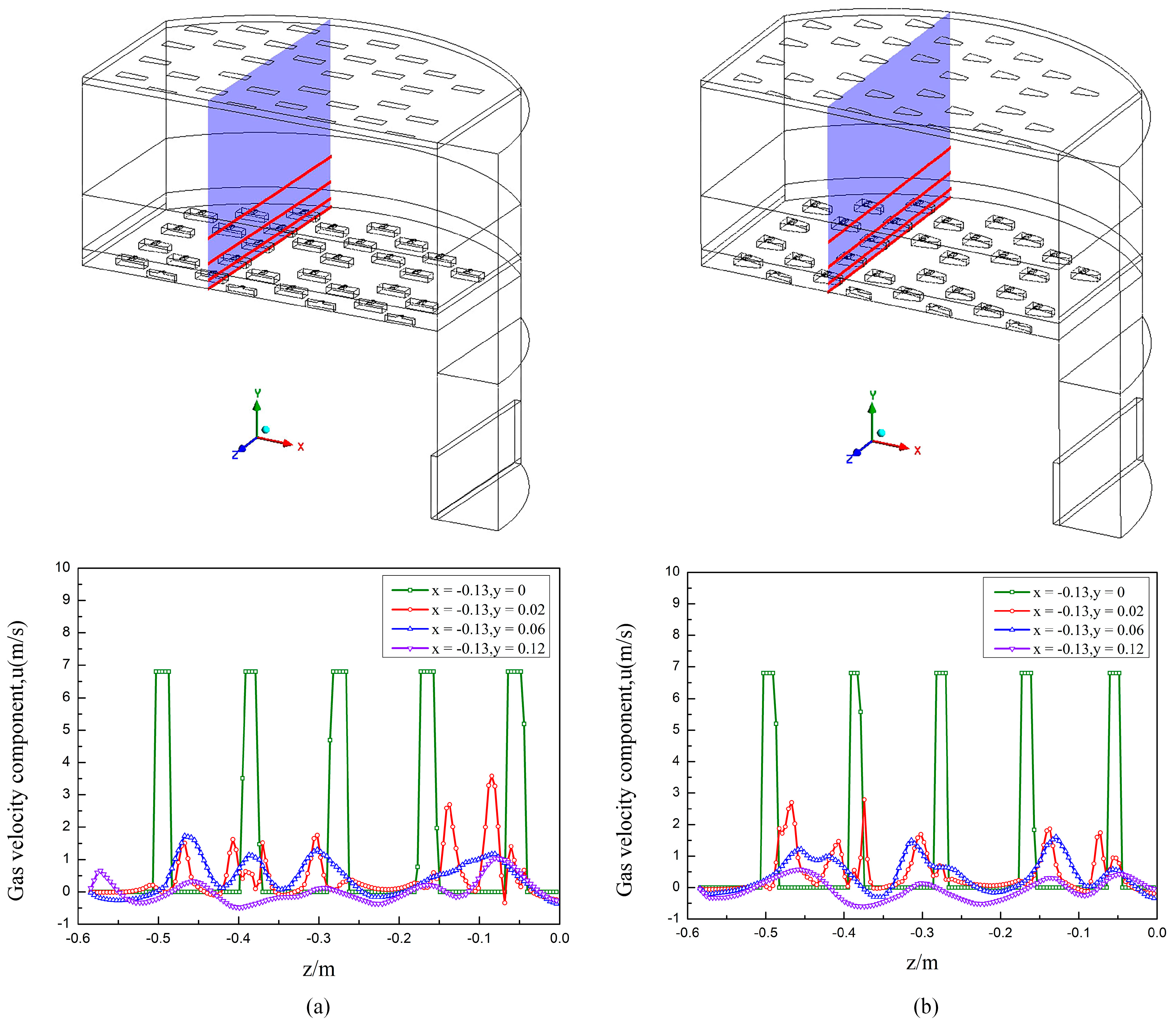
3.3.3. Velocity Distribution of the Gas Phase in the z–Direction

Figure 19 shows the velocity distribution along the z–direction for two valve trays at different heights, taking x = −0.13 m. As seen from the figure, both have a similar trend of variation. In the near–wall region at y = 0, the five peaks of the velocity curve correspond precisely to the openings in the tray, with the remaining part of the velocity dropping to zero. At the height of y = 0.02 m, the gas is ejected from both sides of the valve hole due to the valve cover’s blocking effect, and a gas velocity peak occurs at each side. The insignificant variation in gas velocity between the third and fourth valve holes is because this is the junction of the bowed and rectangular trays, where the valves are sparsely distributed. The remaining small peaks are caused by the gas ejected from the pilot holes. At the height of y = 0.06 m, a peak in gas velocity occurs between the valve holes due to the pronounced hedging effect of the gas flow on both sides of the valve. As the height of the tray increases, the gas crosses the overflow weir and enters the gas phase continuity zone. At y = 0.12 m height, the gas cross–sectional area increases, and the gas velocity decreases significantly.
As can be seen from the graph, the parabolic–shaped guided valve has a lower gas velocity along the y–direction at the same height compared to the rectangular guided valve. The parabolic–shaped guided valve, therefore, has a finer and more homogeneous gas dispersion, which effectively increases the gas–liquid contact area and enhances interphase mass transfer.

3.4. Optimal Design of Parabolic–Shaped Guided Valve Trays

A comparison of the hydrodynamic properties of rectangular and parabolic–shaped guided valve trays shows that parabolic–shaped guided valve trays have a more uniform flow field. However, parabolic–shaped guided valves of different function expressions correspond to different flow field conditions. In order to describe the strength of a valve guide, defined as the ratio of the sum of the velocities at each point along the direction of flow of the main body, at the edge of the bonnet, to half the length of the parabolic arc:
I = u x L
where I is the inflow intensity, ux is the velocity of the liquid phase at any point on the parabola along the direction of flow of the main body, and L is half the arc length of the parabola.
As shown in Figure 20, let the function expression for a parabolic–shaped guided valve be as follows:
y = a x 2
Considering the valve’s mechanical strength and fluid flow performance, the top of the valve is left with a 10 mm leg. The area at the top of the parabola is small and negligible. Then the valve bore area is as follows:
S = 2 t a t 2 2 0 t a x 2 d x = 4 3 a t 3
a = 3 S 4 t 2
where S denotes the area of the valve bore, a denotes the size and direction of the parabola opening, and t denotes half the length of the bottom side of the parabola.
The slope of the tangent line at any point on the parabola is as follows:
d y d x = 2 a x = tan θ
Then the velocity of the liquid phase along the direction of flow of the main body at any point on the parabola is as follows:
u x = u cos θ = u 1 + 4 a 2 t 2 4 a Δ y
where u denotes the velocity of the liquid phase at any point on the parabola, and Δy denotes the distance from the length of the bottom edge at any point on the parabola:
a x 2 = a t 2 Δ y
x = t 2 Δ y a
u x = u 0 h 25 a d Δ y 1 + 4 a 2 t 2 4 a Δ y = u 2 a 1 + 4 a 2 t 2 4 a Δ y 0 h 25 a
where h denotes the distance between the vertex of the parabola and the bottom edge:
h = a t 2
Half of the arc length of the parabola is as follows:
L = 5 t 1 + d y d x 2 d x = 5 t 1 + 4 a 2 x 2 d x
5 t 1 + 4 a 2 x 2 d x = x 1 + 4 a 2 x 2 5 t 5 t 1 + 4 a 2 x 2 d x + 5 t d x 1 + 4 a 2 x 2
2 5 t 1 + 4 a 2 x 2 d x = x 1 + 4 a 2 x 2 + ln 2 a x + 1 + 4 a 2 x 2 5 t
L = 1 2 x 1 + 4 a 2 x 2 + 1 2 ln 2 a x + 1 + 4 a 2 x 2 5 t
Then the inflow intensity is as follows:
I = u 2 a 1 + 4 a 2 t 2 4 a Δ y 0 h 25 a 1 2 x 1 + 4 a 2 x 2 + 1 2 ln 2 a x + 1 + 4 a 2 x 2 5 t
To ensure the same area as the rectangular guided valve:
S = 4 3 a t 3 = 70 25 = 1750
a = 1312.5 t 3
A total of nine sets of a and t values were selected to calculate the inflow strength of each set of parabolic–shaped guided valve trays, the parameters selected and the results are shown in Table 1.
It can be seen that the larger the parabolic opening, the higher the inflow intensity; the smaller the parabolic opening, the lower the inflow intensity. However, as the parabolic opening increases, the length of the bottom edge also increases, which in turn increases the dead zone of the tray and increases re–mixing, affecting the mass transfer efficiency. Therefore, further optimizing the parabolic valve structure to find a parabolic valve structure with optimum performance is necessary.
Then, the nine different valve models of the tray were modeled and simulated. After the convergence of the simulation runs, the liquid phase velocity distribution of the different tray models was quantified. The average liquid phase velocity along the direction of flow of the main body for the nine different models concerning the different heights of the tray is shown in Figure 21.
As can be seen from the graph, the trend of liquid phase velocity along the y–axis is the same for the nine different models. When y < 15 mm, the liquid phase velocity increases monotonically with the y value and reaches its maximum value at the y = 15 mm valve cover. When 15 < y < 55 mm, the liquid phase velocity decreases monotonically with the y value. At y = 55 mm overflow weir, the liquid phase enters the descending liquid pipe and the velocity increases. When y > 55 mm, a significant liquid phase crosses the overflow weir and enters the downcomer. The interaction between the gas and liquid phases is intense, the flow situation is complex, and the liquid phase velocity fluctuates with the y value. Observe the velocity curve of different t values; the liquid phase velocity first increases with the t–value and then decreases. The liquid phase velocity at the bonnet section is increased to a maximum at t = 26. In the region below the overflow weir, the liquid phase velocity is most significant for both t = 24 and t = 26 valve types. In the area above the overflow weir, the liquid phase velocity is most significant for the valve type t = 26 at y < 70 mm. For y > 70 mm, the liquid phase velocity is most significant for the valve type t = 28. As the liquid phase’s main body is the tray’s clear liquid height, liquid phase re–mixing is more severe in the clear liquid height. In contrast, the liquid phase above the clear liquid height is dispersed into droplets, and the direction of movement is disordered and irregular. Therefore, the valve type with high liquid phase velocity in the clear liquid height is the most preferred, and the clear liquid height of all nine valve trays is <70 mm when the calculation is stable. Therefore, the optimal valve configuration is the parabolic–shaped guided valve at t = 26.
Figure 22 shows the liquid phase velocity vector diagrams for the two valve trays at t = 26 and t = 18.5 at y = 15 mm. As can be seen from the graphs, some small vortices are formed around the valve due to the hedging effect of the airflow between the valves. Valves are sparsely distributed at the transition zone between the bowed tray and the channel tray and the bowed zone near the tower wall, and the swirling phenomenon is serious. t = 26 valve has a higher liquid phase velocity than the t = 18.5 valve, with a maximum liquid phase velocity of 6.3 m/s. In addition, as shown by the arrow direction, the t = 26 valve has a higher liquid phase velocity along the main liquid flow direction, effectively reducing the impact of airflow hedging between the valves, reducing re–mixing, and facilitating mass transfer. Therefore, the performance of the parabolic–shaped guided valve with t = 26 is superior.
The gas–liquid phase flow line distribution of the parabolic–shaped guided valve tray at t = 26 at a particular moment after the calculation reaches stability is shown in Figure 23: blue indicates the liquid phase flow line, and yellow indicates the gas phase flow line. As seen from the diagram, the liquid phase moves in the direction of the liquid flow in the column tray, over the overflow weir to the downcomer, and then out through the bottom gap of the downcomer. Due to the gas phase’s stirring and the valve’s guide effect, the liquid phase does not flow straight through, but some swirls will be formed during the flow. The gas phase’s main flow direction is perpendicular to the tray, and its flow line has a significant bend in the gas–liquid transfer zone. Due to the guiding effect of the valve, some gas phase flow lines appear near the exit weir and form a vigorous mixing with the liquid phase. Once the gas phase has passed through the liquid layer, it is unaffected by the valve and will flow in a straight line and out of the top valve hole. The red and green surfaces indicate the equivalent surfaces for liquid phase fractions of 99% and 1%, respectively. As can be seen, most of the liquid phase is concentrated at the bottom of the tray, with a minimal amount of liquid phase distributed above the clear liquid height, indicating that the mist entrainment is also very small for a valve tray at t = 26. The flow lines and isosurfaces visualize the flow inside the tray and help optimize the tray structure’s design.

4. Conclusions

(1)
A new parabolic–shaped guided valve tray is proposed. CFD simulations of the gas–liquid two–phase flow field are carried out for parabolic–shaped and conventional rectangular guided valve trays. The relationship between the superficial gas velocity, liquid flow intensity and weir height and the clear liquid height under different working conditions is described. The simulated values of the clear liquid height are compared with the calculated values of the previous empirical correlations, which agree with each other, thus verifying the correctness of the simulation results.
(2)
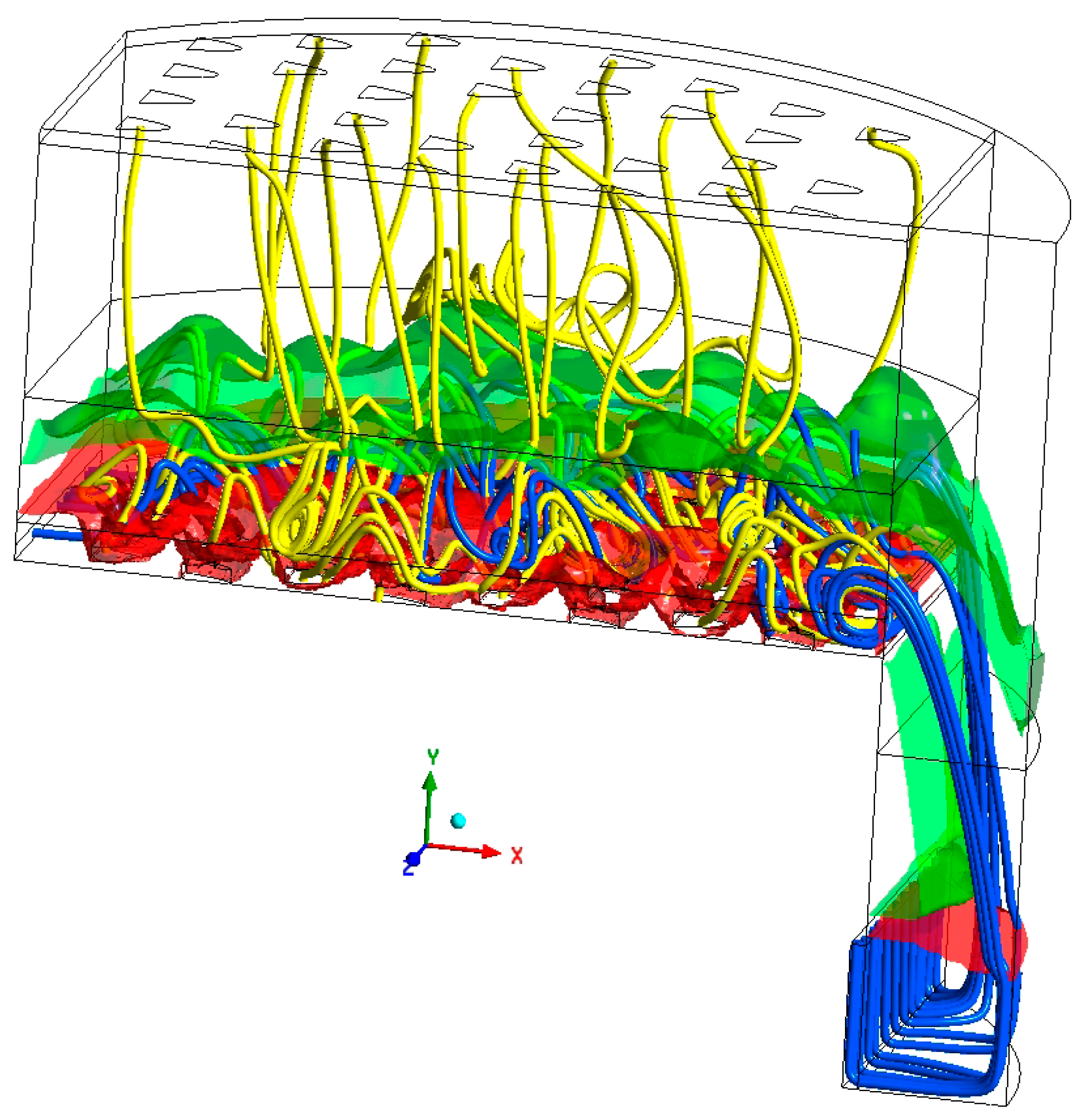
From the simulation results, the phase fraction distribution, the clear liquid height distribution and the two–phase flow velocity field distribution on different cross–sections of the tray can be observed. The trend of the clear liquid height along the x and y axes shows that the parabolic–shaped guided valve tray has a smaller liquid level difference than the rectangular guided valve tray. The velocity vector of the liquid phase in the x–z section shows that the parabolic–shaped guided valve tray has a larger liquid velocity along the main body direction than the rectangular guided valve tray. Therefore, the performance of a parabolic–shaped guided valve is better.
(3)
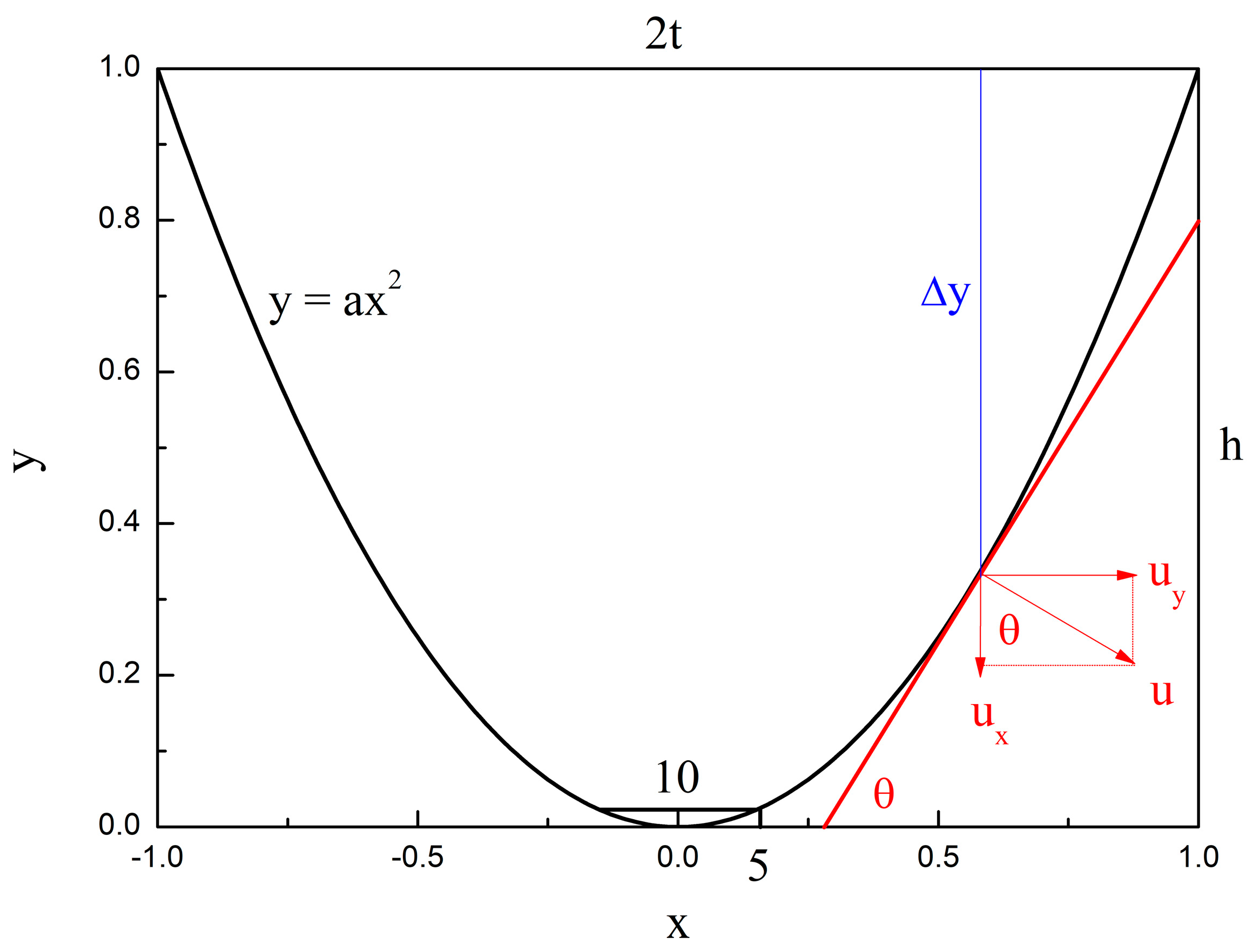
The structural parameters of the parabolic–shaped guided valve are determined by the size of the parabolic opening a and half the length of the bottom side t. Parabolic–shaped guided valve trays for nine different function expressions were modeled and simulated. By comparing the average liquid phase velocity along the direction of flow of the main body at different heights of the tray, the parabolic–shaped guided valve of the a–value at 0.075 and the t–value at 26 is the optimum valve structure.
The simulation of the computational fluid dynamics model overcomes the limitations of the experimental work. It allows for more flexibility in adjusting the structure and operating parameters of the model in completing the optimization design work and saves on equipment costs. The development and analysis of the parabolic–shaped guided valve tray in this paper is a guideline for future optimization of the tray structure.

Author Contributions

Conceptualization, Q.Y.; methodology, C.W.; software, C.W.; validation, Q.Y. and Y.L.; writing—original draft preparation, C.W.; writing—review and editing, Q.Y. and H.S.; visualization, C.W.; supervision, P.Y. All authors have read and agreed to the published version of the manuscript.

Funding

This work was financially supported by the National Natural Science Foundation of China [Nos. 22178113].

Data Availability Statement

Not applicable.

Conflicts of Interest

The authors declare no conflict of interest.

References

  1. Li, X.G.; Liu, D.X.; Xu, S.M.; Li, H. CFD simulation of hydrodynamics of valve tray. Chem. Eng. Process.-Process Intensif. 2009, 48, 145–151. [Google Scholar] [CrossRef]
  2. Zarei, A.; Hosseini, S.H.; Rahimi, R. CFD and experimental studies of liquid weeping in the circular sieve tray columns. Chem. Eng. Res. Des. 2013, 91, 2333–2345. [Google Scholar] [CrossRef]
  3. Zarei, A.; Hosseini, S.H.; Rahimi, R. CFD study of weeping rate in the rectangular sieve trays. J. Taiwan Inst. Chem. Eng. 2013, 44, 27–33. [Google Scholar] [CrossRef]
  4. Zhao, H.K.; Li, Q.S.; Yu, G.Q.; Dai, C.N.; Lei, Z.G. Performance analysis and quantitative design of a flow-guiding sieve tray by computational fluid dynamics. AIChE J. 2019, 65, e16563. [Google Scholar] [CrossRef]
  5. Jiang, S.; Gao, H.; Sun, J.S.; Wang, Y.H.; Zhang, L.N. Modeling fixed triangular valve tray hydraulics using computational fluid dynamics. Chem. Eng. Process.-Process Intensif. 2012, 52, 74–84. [Google Scholar] [CrossRef]
  6. Ma, Y.F.; Ji, L.J.; Zhang, J.X.; Chen, K.; Wu, B.; Wu, Y.Y.; Zhu, J.W. CFD gas-liquid simulation of oriented valve tray. Chin. J. Chem. Eng. 2015, 23, 1603–1609. [Google Scholar] [CrossRef]
  7. Zarei, T.; Farsiani, M.; Khorshidi, J. Hydrodynamic characteristics of valve tray: Computational fluid dynamic simulation and experimental studies. Korean J. Chem. Eng. 2017, 34, 150–159. [Google Scholar] [CrossRef]
  8. Zarei, T.; Rahimi, R.; Zivdar, M. Computational fluid dynamic simulation of MVG tray hydraulics. Korean J. Chem. Eng. 2009, 26, 1213–1219. [Google Scholar] [CrossRef]
  9. Bangga, G.; Novita, F.J.; Lee, H.Y. Evolutional computational fluid dynamics analyses of reactive distillation columns for methyl acetate production process. Chem. Eng. Process.-Process Intensif. 2019, 135, 42–52. [Google Scholar] [CrossRef]
  10. Lavasani, M.S.; Rahimi, R.; Zivdar, M. Hydrodynamic study of different configurations of sieve trays for a dividing wall column by using experimental and CFD methods. Chem. Eng. Process.-Process Intensif. 2018, 129, 162–170. [Google Scholar] [CrossRef]
  11. Rodriguez-Angeles, M.A.; Gomez-Castro, F.I.; Segovia-Hernandez, J.G.; Uribe-Ramirez, A.R. Mechanical design and hydrodynamic analysis of sieve trays in a dividing wall column for a hydrocarbon mixture. Chem. Eng. Process.-Process Intensif. 2015, 97, 55–65. [Google Scholar] [CrossRef]
  12. Roshdi, S.; Kasiri, N.; Hashemabadi, S.H.; Ivakpour, J. Computational fluid dynamics simulation of multiphase flow in packed sieve tray of distillation column. Korean J. Chem. Eng. 2013, 30, 563–573. [Google Scholar] [CrossRef]
  13. Liu, C.J.; Yuan, X.G.; Yu, K.T.; Zhu, X.J. A fluid-dynamic model for flow pattern on a distillation tray. Chem. Eng. Sci. 2000, 55, 2287–2294. [Google Scholar] [CrossRef]
  14. Yu, K.T.; Yuan, X.G.; You, X.Y.; Liu, C.J. Computational fluid-dynamics and experimental verification of two-phase two-dimensional flow on a sieve column tray. Chem. Eng. Res. Des. 1999, 77, 554–560. [Google Scholar] [CrossRef]
  15. Li, Q.S.; Li, L.; Zhang, M.X.; Lei, Z.G. Modeling Flow-Guided Sieve Tray Hydraulics Using Computational Fluid Dynamics. Ind. Eng. Chem. Res. 2014, 53, 4480–4488. [Google Scholar] [CrossRef]
  16. Li, X.G.; Yang, N.; Sun, Y.L.; Zhang, L.H.; Li, X.G.; Jiang, B. Computational Fluid Dynamics Modeling of Hydrodynamics of a New Type of Fixed Valve Tray. Ind. Eng. Chem. Res. 2014, 53, 379–389. [Google Scholar] [CrossRef]
  17. Krishna, R.; van Baten, J.M. Modelling sieve tray hydraulics using computational fluid dynamics. Chem. Eng. Res. Des. 2003, 81, 27–38. [Google Scholar] [CrossRef]
  18. Krishna, R.; Van Baten, J.M.; Ellenberger, J.; Higler, A.P.; Taylor, R. CFD simulations of sieve tray hydrodynamics. Chem. Eng. Res. Des. 1999, 77, 639–646. [Google Scholar] [CrossRef]
  19. Feng, W.; Fan, L.; Zhang, L.; Xiao, X. Hydrodynamics Analysis of a Folding Sieve Tray by Computational Fluid Dynamics Simulation. J. Eng. Thermophys. 2018, 27, 357–368. [Google Scholar] [CrossRef]
  20. Rahimi, M.R. Characteristics of Gas-Liquid Contact on Cross-Current Trays. Sep. Sci. Technol. 2014, 49, 2772–2782. [Google Scholar] [CrossRef]
  21. Troudi, H.; Ghiss, M.; Ellejmi, M.; Tourki, Z. Performance comparison of a structured bed reactor with and without a chimney tray on the gas-flow maldistribution: A computational fluid dynamics study. Proc. Inst. Mech. Eng. Part E—J. Process Mech. Eng. 2020, 234, 83–97. [Google Scholar] [CrossRef]
  22. Krishna, R.; Urseanu, M.I.; van Baten, J.M.; Ellenberger, J. Rise velocity of a swarm of large gas bubbles in liquids. Chem. Eng. Sci. 1999, 54, 171–183. [Google Scholar] [CrossRef]
  23. Bennett, D.L.; Agrawal, R.; Cook, P.J. New pressure drop correlation for sieve tray distillation columns. AIChE J. 1983, 29, 434–442. [Google Scholar] [CrossRef]
  24. Jin, H.B.; Lian, Y.C.; Qin, L.; Yang, S.H.; He, G.X.; Guo, Z.W. Parameters Measurement of Hydrodynamics and Cfd Simulation in Multi-Stage Bubble Columns. Can. J. Chem. Eng. 2014, 92, 1444–1454. [Google Scholar] [CrossRef]
  25. Shenastaghi, F.K.; Roshdi, S.; Kasiri, N.; Khanof, M.H. CFD simulation and experimental validation of bubble cap tray hydrodynamics. Sep. Purif. Technol. 2018, 192, 110–122. [Google Scholar] [CrossRef]
  26. Wang, Y.; Du, S.; Zhu, H.G.; Ma, H.X.; Zuo, S.Q. CFD Simulation of Hydraulics of Dividing wall Sieve Trays. In Proceedings of the 3rd International Conference on Manufacturing Science and Engineering (ICMSE 2012), Xiamen, China, 27–29 March 2012; pp. 1345–1350. [Google Scholar]
  27. Papageorgakis, G.C.; Assanis, D.N. Comparison of linear and nonlinear RNG-based k-epsilon models for incompressible turbulent flows. Numer. Heat Transf. Part B Fundam. 1999, 35, 1–22. [Google Scholar] [CrossRef]
  28. Zakrzewska, B.; Jaworski, Z. CFD modelling of turbulent jacket heat transfer in a rushton turbine stirred vessel. Chem. Eng. Technol. 2004, 27, 237–242. [Google Scholar] [CrossRef]
Figure 1. Model geometry and boundary conditions: (a) rectangular guided valve tray; (b) parabolic–shaped guided valve tray.
Separations 10 00267 g001
Figure 2. Valve structures: (a) rectangular guided valve; (b) parabolic–shaped guided valve.
Separations 10 00267 g002
Figure 3. Illustration of the computation mesh: (a) Whole valve tray space mesh; (b) The bottom mesh of the valve tray.
Separations 10 00267 g003
Figure 4. Transient clear liquid height monitored as a function of time. US = 0.65 m/s, hW = 0.054 m, QL/Lw = 20 m3/(m·h).
Separations 10 00267 g004
Figure 5. Clear liquid height as a function of the superficial gas velocity. hW = 0.054 m, QL/Lw = 20 m3/(m·h).
Separations 10 00267 g005
Figure 6. Clear liquid height as a function of the liquid load per weir length. US = 0.65 m/s, hW = 0.054 m.
Separations 10 00267 g006
Figure 7. Clear liquid height as a function of the weir height. US = 0.65 m/s, QL/Lw = 20 m3/(m·h).
Separations 10 00267 g007
Figure 8. Liquid hold–up snapshots of the front view: (a) rectangular guided valve tray; (b) parabolic–shaped guided valve tray.
Separations 10 00267 g008
Figure 9. Gas hold–up snapshots of the top view at different heights of the rectangular guided valve tray.
Separations 10 00267 g009
Figure 10. Gas hold–up snapshots of the top view at different heights of the parabolic–shaped guided valve tray.
Separations 10 00267 g010
Figure 11. Average gas hold–up at different heights.
Separations 10 00267 g011
Figure 12. The clear liquid height changes in the x–direction.
Separations 10 00267 g012
Figure 13. The clear liquid height changes in the z–direction.
Separations 10 00267 g013
Figure 14. Liquid velocity vector snapshots of the top view at y = 10 mm: (a) rectangular guided valve tray; (b) parabolic–shaped guided valve tray.
Separations 10 00267 g014
Figure 15. Liquid velocity vector snapshots of the top view at y = 15 mm: (a) rectangular guided valve tray; (b) parabolic–shaped guided valve tray.
Separations 10 00267 g015
Figure 16. Liquid velocity vector snapshots of the top view at y = 17 mm: (a) rectangular guided valve tray; (b) parabolic–shaped guided valve tray.
Separations 10 00267 g016
Figure 17. Liquid velocity vector snapshots of the top view at y = 30 mm: (a) rectangular guided valve tray; (b) parabolic–shaped guided valve tray.
Separations 10 00267 g017
Figure 18. The x–direction–component velocity profiles of the liquid flow field at different elevations: (a) y = 0.01 m; (b) y = 0.03 m; (c) y = 0.05 m.
Separations 10 00267 g018
Figure 19. Gas–phase vertical–component velocity at different elevations above tray deck: (a) rectangular guided valve tray; (b) parabolic–shaped guided valve tray.
Separations 10 00267 g019
Figure 20. Curve equation of the parabolic–shaped guided valve.
Separations 10 00267 g020
Figure 21. The mean liquid phase velocity trends with the y–direction for the different models.
Separations 10 00267 g021
Figure 22. Liquid velocity vector snapshots of the top view at y = 15 mm: (a) t = 26; (b) t = 18.5.
Separations 10 00267 g022
Figure 23. Gas–liquid streamline distribution and isosurface.
Separations 10 00267 g023
Table 1. Parameter values of the parabola and inflow strength.
atI
0.0486300.46 u
0.06280.42 u
0.075260.37 u
0.095240.33 u
0.123220.28 u
0.164200.23 u
0.218.50.20 u
0.32160.15 u
0.478140.11 u
Disclaimer/Publisher’s Note: The statements, opinions and data contained in all publications are solely those of the individual author(s) and contributor(s) and not of MDPI and/or the editor(s). MDPI and/or the editor(s) disclaim responsibility for any injury to people or property resulting from any ideas, methods, instructions or products referred to in the content.

