A Novel Surface Parametric Method and Its Application to Aerodynamic Design Optimization of Axial Compressors

Abstract

A novel parametric control method for the compressor blade, the full-blade surface parametric method, is proposed in this paper. Compared with the traditional parametric method, the method has good surface smoothness and construction convenience while maintaining low-dimensional characteristics, and compared with the semi-blade surface parametric method, the proposed method has a larger degree of geometric deformation freedom and can account for changes in both the suction surface and pressure surface. Compared with the semi-blade surface parametric method, the method only has four more control parameters for each blade, so it does not significantly increase the optimization time. The effectiveness of this novel parametric control method has been verified in the aerodynamic optimization field of compressors by an optimization case of Stage35 (a single-stage transonic axial compressor) under multi-operating conditions. The optimization case has brought the following results: the adiabatic efficiency of the optimized blade at design speed is 1.4% higher than that of the original one and the surge margin 2.9% higher, while at off-design speed, the adiabatic efficiency is improved by 0.6% and the surge margin by 1.3%.

1. Introduction

In recent decades, there have been many important developments in compressor aerodynamic optimization design methods. Compared with traditional compressor design methods, the optimization method not only reduces the dependence on expert experience but also overcomes the limitations of traditional design. However, aerodynamic optimization design of compressors has three typical characteristics: high-dimensional, expensive computational cost and black-box, abbreviated as the HEB problem. Since the possible design space of blade geometry rises sharply with the number increase in optimization control variables, the optimization process can easily fall into a “dimensional disaster” [1,2,3]. It is often impossible to obtain an optimal solution within an acceptable amount of time in engineering. How to effectively break through the aerodynamic optimization HEB problem for compressors is one of the research hotspots in this field.

One of the key aspects of the optimization design of compressor blades is geometry parameterization. The parametric method determines the size and structure of the blade geometry deformation space. One of the most promising methods for solving the HEB problem is parametric dimensionality reduction [4]. The objective of this method is to reduce the number of optimal control variables while retaining the optimal solution in the original design space, so as to reduce the design space. For the aerodynamic optimization of compressors, it is an effective way to reduce the dimension by establishing a geometric parametric method of compressor blade with few parameters and good performance. Traditional geometric parametric methods for compressor blades can be divided into three categories. In the first category, the geometry of each radial section remains unchanged, and their axial and circumferential changes are used as control parameters (bow and sweep) of the 3D blade geometry [5,6]. Although this parametric method has fewer control parameters, its approach often leads to excessive modification of the original blade, which is unable to fine-tune the blade geometry, and because most of the optimization objects are blades designed by experts in detail, this parametric method often fails to meet the aerodynamic constraints in the optimization process. Thus, it is rarely used in an actual optimization project. The second category is to take the control parameters of free curves that fit the central arc of the 2D cascade geometry [7,8,9,10] or the profile of the suction and pressure side as optimization variables [11,12,13,14]. These control parameters can control the geometric changes in the 3D blades during the optimization process. The third category is a combination of the first and second parametric methods. The core disadvantages of the latter two traditional methods are the large number of geometric control parameters, the enormous design space and the fact that the parameterization process requires fitting back calculation, which has the problem of fitting accuracy. The recently developed free form deform (FFD) parametric method [15,16,17] is suitable for modeling complex geometry and for local fine-tuning, but still suffers from the disadvantage of too many control parameters in most cases, and most importantly, the method is not geometrically intuitive, which leads to difficulty in obtaining a suitable variable range. In 2003, the semi-blade surface parametric method was utilized by Stephane et al. [18] to modify the shape of the suction surface of a transonic rotor. The semi-blade surface parametric method first regards the blade geometry as a combination of the suction surface and pressure surface, and it is a 3D surface parametric method in the true sense. The parametric method has good low-dimensional characteristics, but also a smooth-shaped surface, and making it easy to ensure the advantages of rotor mechanical strength is one of the important development directions of the compressor blade parametric [19]. However, this method limits the degree of freedom of geometric deformation. The special problems are as follows: (1) the modified area only covers one surface (suction or pressure surface) of the compressor blade. So, the effect of the other surface on the aerodynamic performance cannot be accounted for at the same time; (2) the leading and trailing edges cannot be adjusted. It reduces the geometric exploration ability of this parametric method and greatly reduces the probability of the existence of the optimal solution in the original design spaces.

Aiming at the defects of the semi-blade surface parametric method, this paper proposes a new full-blade surface parametric method and uses this method to parameterize the rotor and stator blade of Stage35. The full-blade parameterization method not only continues the smoothness and convenience of surface parametric control, but also overcomes the shortcomings of the semi-blade parametric method. It takes into account the suction surface and pressure surface of the blade, so that the leading edge and trailing edge of the blade have a certain geometric variability. Thus, this method can broaden the ability of geometric exploration and improve the probability of the existence of the optimum solution in the original design space. An improved artificial bee colony (IABC) algorithm is adopted for global optimization and the strategy of a “coarse grid to optimize and fine grid to analyze” is adopted in the optimization process, to save the time cost. Combined with the verified computational fluid dynamics (CFD) numerical method, Stage35 is aerodynamically optimized under multi-operating conditions, and an optimized solution is obtained within a relatively acceptable engineering time cost. This result verifies the superiority of the optimization method based on the full-blade surface parametric method in exploring an acceptable approach for multistage compressors with constraints and multi-objective optimization.

2. Full-Blade Surface Parametric Control Method

As shown in Figure 1, the full-blade surface parametric method considers the suction and pressure surfaces of the blade as a whole surface and superimposes Bezier surfaces on the entire surface to form a new blade. The control parameters of the Bezier surface are the optimization design variables that control the blade geometry in the optimization cycle, and the deformation of the blade geometry is controlled by the superimposed Bezier surface. During the superposition process, the four vertices of the Bezier surface correspond one-to-one with the four vertices of the original blade surface.

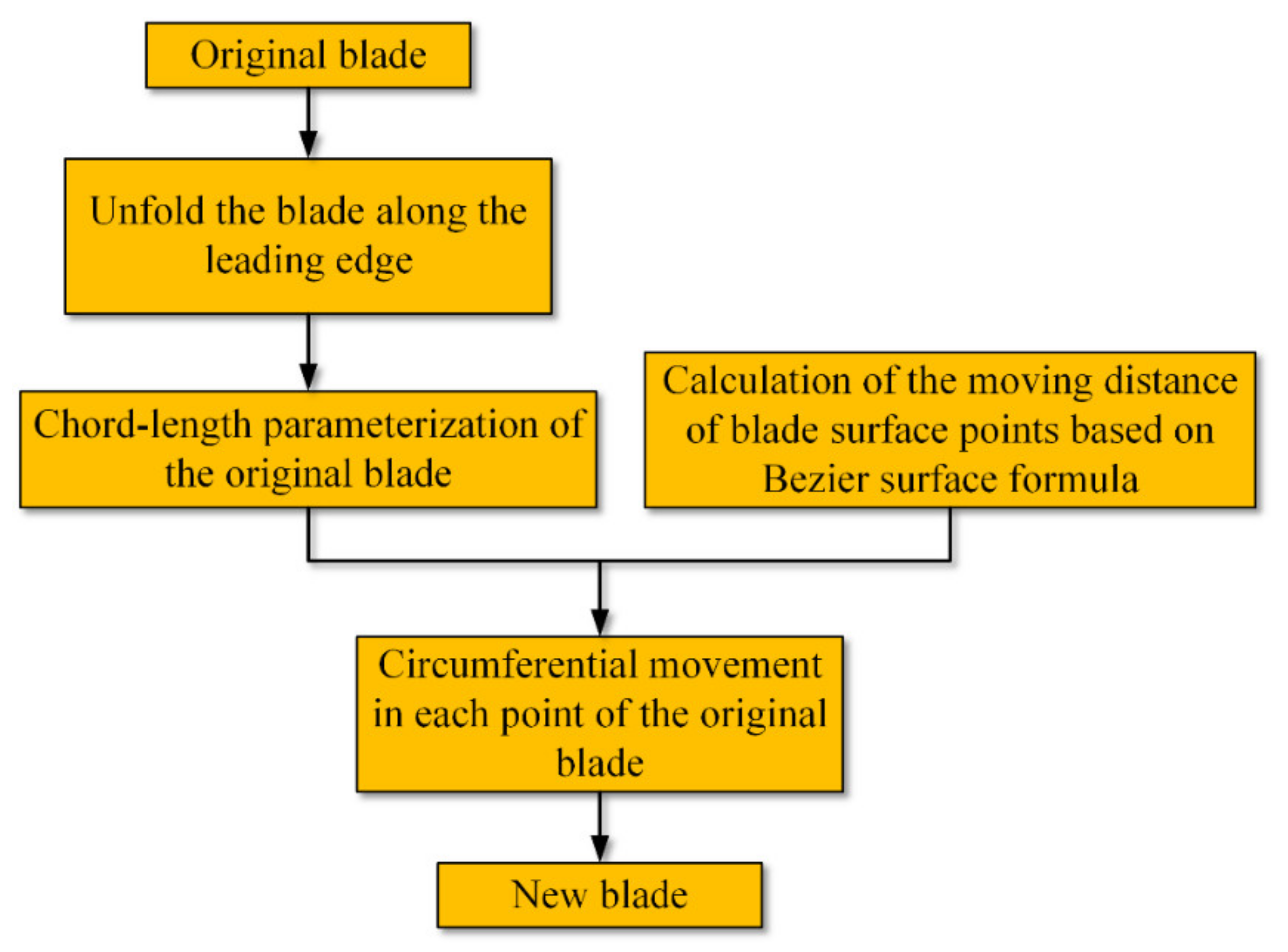
The proposed full-blade surface control parametric method includes the following four steps, as shown in Figure 2:

Step 1. The original blade is unfolded along the radial line of the leading edge. As a result, the trailing edge line becomes the middle position of the unfolded blade surface.

Step 2. Chord length parameterization. Since the Bezier surface is a unit surface in the calculation domain, it cannot be directly covered on the three-dimensional unfolded surface of the original blade. Therefore, in order to correspond each point of the physical domain and the computational domain one by one in the superposition process, each point of profile of the three-dimensional blade unfolded surface must be normalized. The method adopted is chord length parameterization, and it is shown in Equations (1) and (2).

$${\mathsf{\xi }}_{i,j}=\frac{{{\displaystyle \sum }}_{m=1}^{i}l\_c_m}{L\_C_j}$$

(1)

$${\mathsf{\eta }}_{i,j}=\frac{{{\displaystyle \sum }}_{n=1}^{j}l\_s_n}{L\_S_i}$$

(2)

where ${\mathsf{\xi }}_{i,j}$ refers to the horizontal coordinate in the unit domain, and ${\mathsf{\eta }}_{i,j}$ the vertical one. $i\in \left(1,{\mathrm{n}}_p\right),j\in \left(1,{\mathrm{n}}_s\right),{\mathrm{where}\mathrm{n}}_p$means the points of each section profile along the chordwise direction and ${\mathrm{n}}_s$ means the total sections of the blade. $L\_C_j$ refers to the total length of the jth section profile of the blade along the radial direction and $L\_S_i$ the total arc length of the ith profile line of the blade along the chordwise direction. $l\_c_m$ means the length of the mth segment along the arc direction and $l\_s_n$ means the length of the nth segment along the radial direction.

Step 3. Use the Bezier surface generation function to calculate the amount of variation at each point on the computational domain of the unfolded surface of the original blade. The value of the Bezier surface function is determined by Equations (3)–(5).

$$\overrightarrow{R}={\displaystyle \sum }_{k=0}^n\left\{{\displaystyle \sum }_{l=0}^m{P}_{k,l}{B}_l^m\left(v\right)\right\}{B}_k^n\left(u\right)$$

(3)

$$B_k^n\left(u\right)=C_k^n{u}^k{\left(1-u\right)}^{n-k}$$

(4)

$$C_k^n=\left\{\begin{array}{c}\frac{n!}{\left(n-k\right)!k!} if 0\le k\le n\\ 0 if not\end{array}\right.$$

(5)

$\overrightarrow{R}$ in Equation (3) is the function value of the Bezier surface, which represents the circumferential variation distance at each point of the unfolded surface of the original blade. Where $B_l^m\left(v\right)\mathrm{and}{B}_k^n\left(u\right)$ are the Bernstein basis functions, calculated by Equation (4), $u$ and $v$ are two independent variables in the calculation domain of the Bezier surface, and their variation ranges are both in [0, 1]. $P_{k,l}$ is the control vertex of the Bezier surface, and the number of control vertices in the horizontal and radial directions is ($m+1$) and ($n+1$), respectively. The value of $C_k^n$ is obtained from the calculation of Equation (5).

Step 4. The R value is superimposed on the circumference of each point on the original unfolded surface to obtain the new blade.

The full-blade surface parametric method has some outstanding advantages: firstly, there is no need to back-calculate the surface control points and no fitting accuracy problem due to the surface superposition rather than surface fitting. Secondly, the higher-order continuity of the Bezier surface [20] ensures that the new blade surface will be no less smooth than the original one. Finally, it reduces the dimensionality of the design variables and has excellent low-dimensional properties due to its inherent constraints of both chordal and radial control points.

Because the full-blade surface parametric control method is developed from the semi-blade surface parametric control method, it is necessary to compare the two methods. Compared to the semi-blade surface parametric method, the full-blade surface parametric method has differences in three aspects:

(1) The full-blade surface parametric method regards the suction and the pressure surface as a whole one, and the moving distance of the corresponding points of the Bezier surface are superimposed on the unfolded surface of the original blade surface. Then, the suction and the pressure surface are connected along the leading edge to form a new blade.

(2) The moving direction of the points of the original blade is no longer along the normal direction like the semi-blade surface method, but in the circumferential direction, as shown in Equation (6):

$${\mathrm{y}}_{new}=y_{old}+\Delta s$$

(6)

where ${\mathrm{y}}_{new}$ refers to the circumferential value at each point of the new blade, and $y_{old}$ refers to that of the original blade, while $\Delta s$ refers to the moving distance of each point corresponding to the Bezier surface.

(3) As shown in Figure 3 below, the red and green points are the active points in the blade geometry deformation process. To maintain first-order continuity at the connection of the suction edge and pressure edge at the leading edge, it is necessary to maintain the same amount of change of the green points at ${\mathsf{\xi }}_1$, ${\mathsf{\xi }}_2$, ${\mathsf{\xi }}_6$, and ${\mathsf{\xi }}_7$. The synchronous changes of the green points cannot change the shape of the leading edge, but it can change the inlet metal angle, which affects the airflow performance. Since the aerodynamic performance of the blade is sensitive to the leading edge geometry, denser control points are required at this region.

The above three differences bring corresponding advantages to three aspects of the full-blade surface parametric method: (1) both the suction and the pressure surface can be parameterized to deform the blade geometry without significantly increasing the number of optimization control variables. (2) It has good parametric reshaping capability for the leading part, which provides the freedom of deformation of this region. (3) Because the circumferential surface superposition direction is driven by the leading edge modification, the geometric changes of the blade body and trailing edge are larger than that of the semi-blade surface method, which makes it easier to break through the design limitations of the original blade.

3. 3D Blade Optimization

3.1. Optimization Case

To verify the effectiveness of the full-blade surface parametric method in solving the HEB problem of the aerodynamic optimization of compressors, a global optimization engineering task was built on a commercial supercomputing platform, which contains three parts: the full-blade surface parametric method, IABC algorithm and CFD flow field calculation program and the general single-stage axial flow transonic compressor Stage35 was selected as the test case to obtain the optimized compressor blade shape under multi-operating conditions at design speed and off-design speed (N = 0.8).

Reference [21] gives detailed information about the geometric data and experimental data of Stage35. Stage35 has a low aspect ratio and was designed by NASA in 1978 [21], and the rotor and the stator blade have 36 and 46 multiarc blades, respectively.

3.2. Parameter Setting of Blade Parameterization

The key to engineering optimization design of compressors is to balance the design space against the computational cost. As the design space increases exponentially with the number of optimization variables, it is easy to fall into a “dimensional curse” that can lead to the failure of the optimization. Actually, the engineering optimization requires that the optimization variables are minimized while ensuring sufficient design space. In other words, the parametric method needs to ensure the low-dimensional characteristics.

In the literature [18,19], the semi-blade surface parametric method only selects the suction surface as an optimization object; however, this selection is applicable only to the case in which the loss of the suction surface far exceeds that of the pressure surface, while the influence on the aerodynamic performance of both the surfaces is accounted for by the full-blade surface parametric control method. In principle, the number of control points can be increased with the improvement of control accuracy. However, due to the global deformation characteristics of the Bezier surface, too many control points easily interfere with each other and increase the design space. As a rule of thumb, seven points in the chordwise direction is sufficient to control the geometric deformation, but the number of control points in the radial direction can be increased as needed. In this case, the $6\times 3$ order (seven points chordal, four points radial) Bezier surface is adopted to parameterize the rotor and stator blades of Stage35 by the full-blade surface parametric method. The distribution of control variables is shown in Figure 3. Seven points are distributed in the chordwise direction of the unfolded blade surface. Their positions are 0.0, 0.1, 0.3, 0.5, 0.7, 0.9 and 1.0, respectively. Four points are set along the radial direction of the blade. Due to the large flow loss of the end wall in the hub area, it is necessary to set up some dense devices in the hub area, with relative positions of 0.0, 0.2, 0.5 and 1.0. The range of the optimization variables must be appropriate. If it is too small, it will be difficult to break through the limitations of the original blade geometry. If it is too large, it will easily exceed the requirements of flow rate and pressure ratio. According to trial and error, the variation range of the optimization variable should be set to [−6.0, 6.0] mm. Due to the tangents of the endpoints of the Bezier surface, to keep the first-order continuous smoothness of the leading edge during the geometric modification, the first two points and the last two points in the $\mathsf{\xi }$ direction of the suction and pressure sides must be changed in step. Therefore, the total number of optimization variables of a single blade row is $3\times 4+1\times 4=16$, and in the traditional parametric method of directly fitting the suction and pressure surface, the number of control parameters of a single blade row is about 60 [22]. Even if the thickness distribution is not changed, but only the mean camber line of the four radial cross-sections is used for modification, about 30 parameters are required, and it is not easy to ensure the radial smoothness. The essence of the Bezier surface parametric modification is that each control point of a different cross-section is radially constrained in the same way, resulting in a radially smooth surface on the one hand and a smaller design space on the other.

3.3. Optimization Algorithm

The use of adjoint algorithms and surrogate modeling techniques is an important solution to the HEB problem of the compressor aerodynamic optimization. At the end of the 1980s, the adjoint algorithm rose and developed rapidly in the field of aerodynamic optimization design [23,24]. Soon, this new method was valued by researchers in the field of turbomachinery, and achieved a lot of research results [25,26,27]. The adjoint method has an obvious advantage that the calculation cost of the optimization has nothing to do with the number of optimization variables, and the gradient of each design variable can be quickly obtained by solving the adjoint matrix, and the sensitivity of each variable can be obtained. However, the disadvantages are that the optimization results are only localized, and it is difficult to deal with multiple constraints and multiple objectives [28]. The essence of the surrogate model method is to train the samples in the design space to obtain a fitting function that can be calculated quickly, so as to greatly reduce the computational cost [29,30,31]. However, this method has two defects: first, the samples required for a sufficient precision surrogate model increases sharply with the increase in the number of optimization variables, which itself costs a lot of computational time, so it is not suitable for high-dimensional problems; second, in high-dimensional problems, the difficulty of sample fitting is greatly increased, even if the sample size is sufficient; it is also difficult to obtain accurate surrogate functions, and it is easy to give wrong optimization solutions. In recent years, deep reinforcement learning has been applied in the field of engineering optimization [32]. This method is a combination of deep learning and reinforcement learning, and has good perception ability and decision-making ability. However, this method has not been well applied to the aerodynamic optimization of 3D blades.

The evolutionary algorithm is a widely used method in the field of engineering optimization [33,34,35], which has good robustness and global convergence. For a better global search, the optimization process uses the IABC algorithm proposed in the literature [36]. The IABC algorithm is used because it has the following three advantages: (1) the IABC algorithm is global, robust, and does not depend on the initial solution; (2) each generation of individuals is independent of each other, which allows for multitask concurrency and shortens optimization time by taking advantage of the enormous computational power of commercial supercomputing platforms [37]; (3) compared to general-purpose genetic algorithms and standard artificial bee colony (ABC) algorithms, the IABC algorithm has better global search and fast convergence capability. Meanwhile, its disadvantage is that the convergence of this method requires more iterations than the adjoint algorithm and surrogate technology. However, engineering optimization often does not focus on the global convergence solution; it needs to obtain the relative optimal solution to meet the engineering requirements in an acceptable time range. Therefore, the IABC algorithm should be used as the optimization algorithm, and the time to jump out of the cycle can be determined by the designer (usually set the upper limit of the number of times for bees to explore food sources). The IABC algorithm is outlined below.

In the ABC algorithm, both onlooker and employed bees explore new food sources in the way shown in Equation (7), but the equation only uses local random information about the bees. The IABC algorithm is improved by using a formula that explores new food sources for employed bees with global best information by Equations (8) and (9) with local best information for onlooker bees.

$$V_i^j=X_i^j+{\phi }_i^j\left(X_i^j-X_k^j\right)$$

(7)

$$V_i^j=X_i^j+{\xi }_i^j(X_i^j-X_k^j)+1.5{\lambda }_i^j(X_{\mathit{best}}^j-X_i^j)$$

(8)

$${(V_{Neib}^j)}_{best}={(X_{Neib}^j)}_{best}+{\xi }_i^j({(X_{Neib}^j)}_{best}-X_k^j)$$

(9)

where $V_i^j$ indicates the location of the new food source explored by the employed bee, ${\xi }_i^j$ and ${\lambda }_i^j$ are random numbers between [−1, 1], $X_i^j$ refers to the jth component of the i-th individual, and $X_{best}^j$ is the best fitness location among successive generations of food sources. ${(X_{Neib}^j)}_{best}$ represents the best fitness location within the neighborhood, and ${(V_{Neib}^j)}_{best}$ represents a new food location explored by the onlooker bees; the local best information in Equation (9) requires the Chebyshev distance, which is expressed in Equation (10) as follows:

$$d\left(i,t\right)=\underset{q\to +\infty }{\lim }{\left({\displaystyle \sum }_{j=1}^D{\left|X_i^j-X_t^j\right|}^q\right)}^{1/q}$$

(10)

where$j\in \left\{1,2,\cdots ,D\right\}$,$d\left(i,t\right)$ is the Chebyshev distance between $X_i$ and $X_t$.

The neighborhood of $X_i$ is determined by Equation (11), which shows that $X_t$ is in the neighborhood of $X_i$ when the Chebyshev distance between $X_i$ and $X_t$ is less than or equal to the product of the neighborhood radius r and the average Chebyshev distance, and not otherwise.

$$\left\{\begin{array}{c}d\left(i,t\right)\le r\ast m{d}_i, t\in S\\ d\left(i,t\right)\ge r\ast m{d}_i, t\notin S\end{array}\right.$$

(11)

where $m{d}_i$ is the average Chebyshev distance between $X_i$and the entire onlooker bee population, S is the neighborhood of $X_i$, and r is the radius of the neighborhood and experience shows that the algorithm converges best when r is 1.

${\left(X_{Neib}\right)}_{best}$ is computed from Equation (12).

$$fit\left[{\left(X_{Neib}\right)}_{best}\right]=max\left\{\begin{array}{c}fit\left[{\left(X_{Neib}\right)}_1\right],\\ fit\left[{\left(X_{Neib}\right)}_2\right],\cdots ,\\ fit\left[{\left(X_{Neib}\right)}_S\right]\end{array}\right\}$$

(12)

where fit() is the fitness value of each individual bee.

After the benchmark function test, the IABC algorithm has better global search accuracy and convergence speed than the ABC and GA algorithms, details of which can be found in Ref. [32]. In this case, the bee colony size of the IABC algorithm is 80, the size of bee colony generations is 20, and the upper limit of exploiting times is 3. A total of approximately 1700 calculations is performed on a commercial supercomputing platform. Each optimization task requires seven cores in parallel. A maximum of 24 tasks can be concurrently performed at one time. The time to complete each optimization task is 15 min, and the total optimization time is 48 h.

3.4. Objective Function and Constraints

To further reduce the optimization time, according to experience, it is often possible to improve the adiabatic efficiency and surge margin by choosing the optimization operating point between the design point and the near-surge point. Therefore, 140,000 pa back pressure at design speed is selected as optimization operating point 1, and 120,000 pa back pressure at off-design speed (N = 0.8) is selected as optimization operating point 2. The multi-objective optimization adopts the weighted summation method, and the optimization objective function is expressed as shown in Equation (13):

$$\max f={\mathsf{\omega }}_1\ast {\mathrm{f}}_1+{\mathsf{\omega }}_2\ast {\mathrm{f}}_2$$

(13)

The constraint conditions are shown in Equation (14):

$$\begin{array}{c}{\mathrm{f}}_1=ef{f}_1;\mathrm{if}\left\{\begin{array}{c}\left|\frac{{\mathrm{mass}}_1-{\mathrm{mass}}_1^{\mathrm{ori}}}{{\mathrm{mass}}_1^{\mathrm{ori}}}\right|\le 0.5\%\\ {\mathrm{TPR}}_1-{\mathrm{TPR}}_1^{\mathrm{ori}}\ge 0\end{array}\right.\\ {\mathrm{f}}_2=ef{f}_2;\mathrm{if}\left\{\begin{array}{c}\left|\frac{{\mathrm{mass}}_2-{\mathrm{mass}}_2^{\mathrm{ori}}}{{\mathrm{mass}}_2^{\mathrm{ori}}}\right|\le 0.5\%\\ {\mathrm{TPR}}_2-{\mathrm{TPR}}_2^{\mathrm{ori}}\ge 0\end{array}\right.\\ {\mathrm{else}\mathrm{f}}_1=\mathrm{minus}\\ {\mathrm{f}}_2=\mathrm{minus}\\ x_i^L\le {\mathrm{x}}_i\le x_i^U\end{array}$$

(14)

where $ef{f}_1$ and $ef{f}_2$, respectively, refer to the isentropic efficiency at design speed and off-design speed, ${\mathsf{\omega }}_1$ and ${\mathsf{\omega }}_2$ represent the weighting factor of isentropic efficiency at the two rotating speeds, and ${\mathsf{\omega }}_1$ and ${\mathsf{\omega }}_2$ are all set to 0.5, while ${\mathrm{TPR}}_1$ means the total pressure ratio and ${\mathrm{TPR}}_1^{\mathrm{ori}}$ means the original total pressure ratio, ${\mathrm{mass}}_1$ refers to the updated flow rate and ${\mathrm{mass}}_1^{\mathrm{ori}}$ refers to the original flow, minus represents the minimum artificially given value, ${\mathrm{x}}_i$ means the design variable. $x_i^L$, $x_i^U$ refer to the lower and upper variation limits, respectively.

The maximization of a weighted sum of the isentropic efficiency of the operating conditions at design speed and off-design speed is taken as the optimization goal. The strong constraint conditions are set as follows: the relative variation of the flow rate of the new blade must not exceed 0.5% higher than that of the original one, and the total pressure ratio must be raised. If the requirements are not satisfied, then the objective function f is set to a minimum value to exclude this food source in the optimization process. In the case of strong constraints, in order to generate more feasible solution space, more bees should be adopted to enhance the exploration ability of the algorithm.

3.5. Numerical Method

Flow field calculation is an important part of performance evaluation in the optimization process. The CFD evaluation tool used is the Fine-Turbo module of the commercial software Numeca. The CFD calculation parameters are set as follows: the turbulence model is selected as the S-A one-equation model, the mixed plane method is used for the interface between rotor and stator, the fourth-order Runge–Kutta method is used to perform the time discretization, the central difference method is used to perform the spatial discretization, and the artificial viscosity is used to eliminate the shockwave. Multigrid technology and implicit residual error scheme is set up to accelerate convergence.

The S-A turbulence model has been successfully applied in engineering. Although it is a one-equation model, its accuracy is not inferior to that of the two-equation model. In addition, the S-A turbulence model is not derived and simplified from the two-equation model, but directly derived and modeled step by step by using experience and dimensional analysis. It has three advantages: (1) unlimited grid form and topology; (2) the near-wall region requires fewer mesh points; (3) good numerical stability and convergence.

As shown in Figure 4, the inlet boundary conditions of the calculation are set as follows: the total pressure is set as 101,325 pa, the total temperature 293.15 K, and the incoming airflow direction axial, the non-slip boundary condition is used for the wall, the non-reflecting 2D condition is used for the rotor/stator interface. The outlet boundary conditions are set as follows: the average static pressure is given at the exit, and in the process of simulation, the back pressure gradually is changed from low (choked point) to high (surge point).

3.5.1. Numerical Method Verification

For the purpose of accurate simulation, verifying the accuracy of the numerical simulation is a necessary step before optimization. Here, the above-mentioned Stage35 with detailed experimental data is selected as a case to perform this verification. Figure 5 compares the pressure characteristic line and efficiency characteristic line obtained by simulation with the experimental value. From the comparison of the pressure characteristic line, we can note that the maximum pressure ratio of the experiment is 3.7% higher than the calculated value, while the experimental value of the choked flow is 1.4% lower than the calculated value. For the efficiency characteristic line, the experimental value of the highest efficiency is larger than the calculated value. At the same time, the experimental value of the surge margin is 8% larger than the calculated value. It is analyzed that the relative error between CFD calculation and experimental data is caused by the turbulence model and oscillation error near stall point, especially the flow deviation near stall point. However, on the whole, the change trend of the experimental values and the calculated values are consistent, and the flow field analysis is not at the stall point. Relatively speaking, it has a good calculation accuracy, which ensures the reliability of the flow field calculation in the aerodynamic optimization cycle.

Although there is still a difference gap between the calculated value and the experimental value, the focus of this paper is to verify the optimization method. The verification of the optimization method is mainly based on the calculated performance comparison before and after optimization. It should be noted that we use simulation calculation before and after optimization, and the grid template and calculation parameter settings of the simulation are exactly the same. This is actually a comparison between the two simulated values before and after optimization, which has little to do with the difference between the simulated and experimental values. Therefore, we can consider that the simulation used in this paper can be used to measure the performance of the optimization method. In the field of turbomachinery design optimization, the calculation and comparison method are common.

3.5.2. Grid Setting and Independence Verification

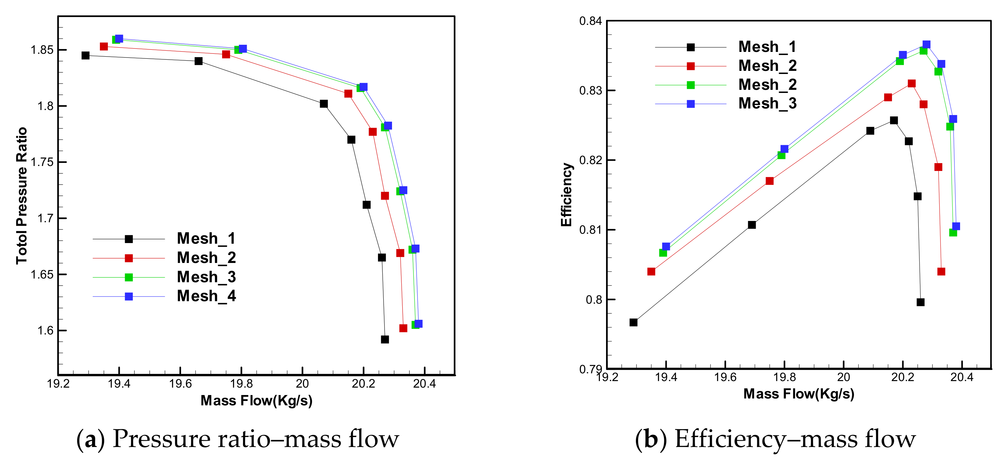
The above general case Stage35 is also utilized to perform the grid independence verification and its grids are automatically generated by the AutoGrid5 module of the commercial software Numeca. The mesh details are shown in Figure 6. The grid generation parameters are set as follows: the first layer grid spacing to 0.001 mm to ensure that the first layer grid $y^{+}\le 5$, the rotor blade tip clearance to 0.408 mm, the stator blade hub clearance to 0.4 mm, and the grid topology 4HO.

The higher the quality of grid, the higher the accuracy of flow field calculation. At the same time, the higher the number of grid, the longer the convergence time of flow field calculation. Therefore, before the actual optimization process, it is necessary to make a trade-off between the quality and quantity of the grid [38,39]. As shown in Figure 7, four sets of different grid templates are utilized to generate the grid for Stage35. The main difference of these grid templates is the grid density, while guaranteeing the quality of each set of grids to meet the calculation requirements. The scale of the four sets of the rotor blades are 320,000, 680,000, 1,020,000 and 1,840,000, respectively, and the grid numbers of stator blades are 340,000, 750,000, 1,100,000 and 1,880,000, respectively. It is obvious that the performance of the third set of grids is very close to that of the fourth set, so the third set of grids is accurate enough to be adopted to calculate the flow field.

In order to ensure both a certain computational accuracy and to save computational cost, this paper adopts the method of “coarse grid optimization and fine grid verification” [40,41], in which the second set of grids is used for the optimization and then the third set of grids is used for the flow field analysis. As a result, it can save about 1/3 of the time.

3.6. Optimization Process

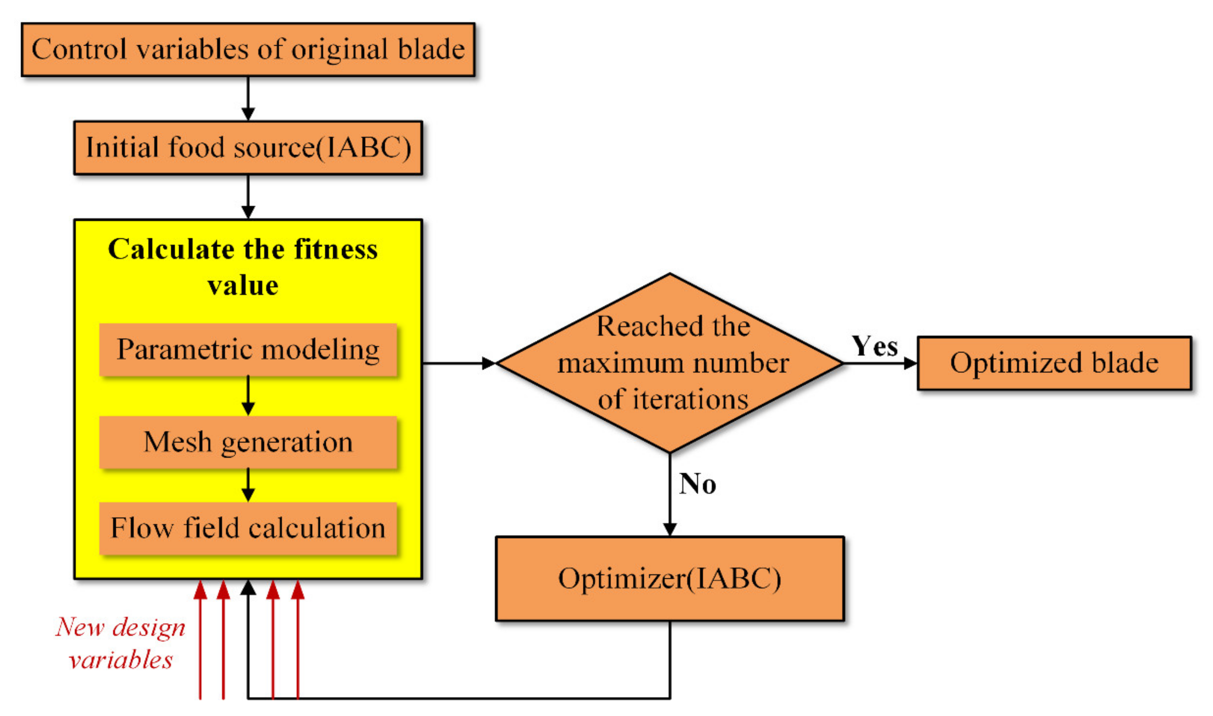
Figure 8 clearly shows each step of the optimization process. The first step is to read the design variables of blade geometry as input parameters, then initialize the food source (design space) to obtain the initial solution in the design space, and then calculate each fitness value. The calculation function of fitness value contains three parts: parametric modeling, mesh generation and flow field calculation. When the performance of the new blade is good enough, the optimization loop finishes, and then the optimal blade geometry is output; otherwise, the optimization algorithm (IABC) will be used to explore the new design space and give a new feasible solution. All above steps complete an iteration. This cycle is followed until the jump out condition (the upper limit of generation times) is satisfied, and then the iteration is completed to obtain the optimized blade.

4. Results and Discussion

4.1. Comparison of Results

Figure 9 shows the optimization history of Stage35 under the multi-operating conditions. The red points are the feasible points in the optimization process, and the blue points represent the Pareto points. Due to the priority of the optimization at design speed, the green point is selected as the final optimal point.

Table 1. Comparison of the performance of original and optimized blade at design speed.

At Design Speed	Flow Rate (kg/s)	Total Pressure Ratio	Adiabatic Efficiency	Surge Margin
Original blade	20.25	1.813	0.837	5.6%
Optimal blade	20.20	1.810	0.851	8.5%
Relative change	−0.25%	−0.17%	+1.4%	+2.9%

and

Table 2. Comparison of the performance of original and optimized blade at off-design speed.

At Off-Design Speed	Flow Rate (kg/s)	Total Pressure Ratio	Adiabatic Efficiency	Surge Margin
Original blade	16.35	1.439	0.847	14.8
Optimal blade	16.36	1.442	0.853	16.1
Relative change	+0.06%	+0.21%	+0.6%	+1.3%

show the comparison of the performance of Stage35 for the working point at design speed and off-design speed before and after optimization. It can be noted from Table 1 that at design speed, the adiabatic efficiency of the optimized blade is 1.4% higher, and the surge margin 2.9% higher, while ensuring that total pressure ratio and the flow rate do not exceed the constraint. As seen from Table 2, at the off-design speed and working point, the adiabatic efficiency improves by 0.6%, and the surge margin by 1.3%.

As shown in Figure 10, the performance of the optimized blade at the design point is not the highest, and the peak efficiency is reached at a higher back pressure. At the back pressure above the peak efficiency point, the optimized efficiency improves by an average of 2%. Overall, the flow rate range of the optimized compressor is reduced, but the comprehensive surge margin (including the effect of pressure ratio) is still improved. At off-design speed, the adiabatic efficiency of the optimized blade above the back pressure of the working point is higher, which not only improves the optimized efficiency at the working point but also broadens the comprehensive surge margin.

Figure 11 shows the corresponding position of each control parameter. Combined with

Table 3. Change value of the design variables.

R_LE_1	−3.46 mm	R_P11	−2.56 mm	R_P21	4.01 mm	R_P31	4.77 mm
R_LE_2	−4.50 mm	R_P12	−1.08 mm	R_P22	5.73 mm	R_P32	4.55 mm
R_LE_3	4.25 mm	R_P13	−4.44 mm	R_P23	3.54 mm	R_P33	0.12 mm
R_LE_4	−2.48 mm	R_P14	0.97 mm	R_P24	−1.91 mm	R_P34	4.20 mm
S_LE_1	1.71 mm	S_P11	−1.41 mm	S_P21	1.25 mm	S_P31	−5.83 mm
S_LE_2	2.20 mm	S_P12	0.59 mm	S_P22	−2.21 mm	S_P32	2.19 mm
S_LE_3	−1.16 mm	S_P13	−5.14 mm	S_P23	5.67 mm	S_P33	3.53 mm
S_LE_4	3.21 mm	S_P14	2.07 mm	S_P24	−0.73 mm	S_P34	−1.50 mm

, we can know the change value of each design variable after optimization, where “R_” refers to the design variables of rotor blades, and “S_” refers to the design variables of stator blades.

Figure 12 shows the comparison of geometric changes of the rotor and stator blade before and after optimization, and the cloud chart shows the distribution of variation values of each point on the unfolding surface. It can be seen from the figure that the leading edge angle of the optimized rotor blade at the hub and tip region increases, and it changes slightly in the blade body. In the region from the hub position to the radial 70% position of the rotor blade, the rear half of the airfoil is convex to a certain extent, which reduces the camber angle of the corresponding airfoil, especially at the 30% radial position. The comparison also shows that the leading edge angle of the optimized stator blade increases significantly, thus leading to the larger camber angle of the airfoil, and the tip region of the blade has the most significant geometric change. It is also found that the blade thickness at the tip and hub of the rotor and stator blade becomes thinner. However, this paper only considers the aerodynamic performance, and does not consider the strength for the time being.

4.2. Analysis of the Optimization Results

4.2.1. Analysis of the Optimization Results at Design Speed

As shown in Figure 13, at design speed, the performance improvement of the optimized rotor is mainly concentrated in the radial region from 10% to 85% of the blade, and the performance is reduced at the tip and hub region of the rotor blade. Meanwhile, it is also noted from the comparison that the performance of the stator blade is not changed as much as that of the rotor blade after optimization. Figure 13b shows that the total pressure ratio decreases in the remaining regions of the rotors except for the 25–50% leaf height region, which remains unchanged.

From the limit streamline comparison shown in Figure 14, it can be seen that the separation line on the suction surface of rotor blade is extended at the hub, but the separation line as a whole is significantly pushed to the trailing edge, so that the separation loss in the hub region of the optimized blade increases, while the separation loss in the area above the hub decreases.

The same conclusion can be drawn from the entropy distribution shown in Figure 15 and Figure 16 as above. From Figure 15, it can be seen that the high entropy region becomes larger in the hub and tip region of the optimized blade, while the entropy value decreases and the flow is smoother in the main flow channel at 10–80% of the blade span. From Figure 16c, the entropy value of the suction surface at 0.95 of blade span is relatively high, which is due to the complex flow situation in this region where there is a leakage vortex interacting with the main flow.

To further analyze the reasons for the decrease in efficiency at the hub and tip of the rotor blade and the increase in efficiency in the middle region, we intercepted the Mach number of the B2B surface before and after optimization, shown in Figure 17, and the static pressure distribution before and after optimization, shown in Figure 18, for comparative analysis. From Figure 17, it can be seen that in the hub region of the optimized blade, the shock wave position on the suction surface is significantly pushed back, but the separation area near the trailing edge after the shock wave is significantly increased, thus increasing the separation loss there. Combined with Figure 12 and Figure 18a, it can be seen that the reason for the above phenomenon is as follows: the increase in the leading edge blade angle at the hub and the camber angle of the optimized rotor blade reduce the positive incidence angle of the incoming flow. It makes the airflow on the suction surface of the acceleration region longer, so that the pressurization region after the shock wave shortens and the reverse pressure gradient increases. As a result, it increases the airflow separation region and increase the corresponding separation loss. Therefore, the airflow turning angle at the hub does not increase, so the total pressure ratio still decreases slightly although the camber angle at the hub of the rotor blade increases. The airflow development in the tip channel of the blade is similar to that in the hub. For the middle section of the blade, the pushing back of the shock wave does not increase the reverse pressure gradient. This is because the camber angle of blade middle geometry is reduced. In this case, the separation region after the shock wave decreases and the corresponding loss decreases.

As shown in Figure 19, the low-energy fluid flows from the pressure surface through the tip gap into the suction surface and sinks at the leading edge, mixing with the main flow in the channel, curling up the leakage vortex and progressing toward the trailing edge and the pressure surface of the adjacent blade. In this process, there is a complex interaction between the secondary flow at the end wall and the leakage vortex. As can be seen from Figure 19, the tip leakage vortex dispersion angle of the optimized blade is smaller, more airflow can rotate to reach the channel outlet, reducing the corresponding airflow loss. Additionally, more leakage vortices in the original blade channel will collide with the pressure surface of the adjacent blade; thus, the loss is larger. At the same time, the leakage vortex rotational strength of the optimized blade is smaller, and the corresponding viscous dissipation loss and mixing losses are also reduced.

At design speed, although the loss of the tip leakage vortex of optimized rotor blade decreases, it is secondary to the loss increase in separation region after the shock wave, so the overall efficiency of the tip section decreases. In contrast, the increase in losses at the hub and tip of the optimized rotor blade is secondary to the increase in efficiency in the middle region, so that the overall performance of the design point is improved at design speed.

4.2.2. Analysis of the Optimization Results at Off-Design Speed

As shown in Figure 20a, the efficiency of the stator blade at off-design speed changes little before and after the optimization, which is the same as design speed, so the next analysis focuses on the rotor blade. In addition to the reduction in the efficiency in the 15~35% height of the rotor blade, the efficiency in other parts of the optimized rotor blade has been improved, and the optimization effect at the 90% height of the rotor blade is the best. It can be seen from Figure 20b that the total pressure ratio at 30–75% of the blade span of the optimized rotor blade is slightly increased, while the total pressure ratio at 75–95% of the blade span is slightly decreased.

From the limit streamline on the suction surface of the rotor blade in Figure 21, the limit streamline after optimization is significantly shortened and the separation line in the 0–40% region of blade span disappears, so the corresponding separation loss is reduced. It can be observed that there is a reattachment line on the suction surface before and after optimization, which is due to the presence of separation bubbles on the suction surface of the rotor blade due to the large positive incidence angle of the incoming flow at off-design speed. The presence of the separation bubble means that there is a separation loss here, and at 60–70% of the blade span, the optimized separation bubble increases, increasing the corresponding airflow loss there.

The flow field at off-design speed is analyzed in more depth by combining the Mach number of B2B surface in Figure 22 and the surface static pressure distribution in Figure 23. The Mach number at the leading edge at the hub and tip of the optimized rotor blade reduces, which weakens the shock wave intensity at this location, leading to a reduction in the corresponding losses of the shock wave as well as the losses from the interaction between the shock wave with the boundary layer. We also note that the separation area at the trailing edge of the rotor blade hub is reduced after optimization, and thus, the corresponding separation losses are reduced. For the middle section, the intensity of the shock wave at the leading edge of the optimized blade increases, and the corresponding shock wave loss increases. At the same time, the positive incidence angle of the incoming flow in the middle of the rotor blade increases, but the camber angle and the trailing edge backward angle of the blade do not change much here. This will increase the turning angle of the airflow and the corresponding rim work, so the total pressure ratio increases there.

Then, we study the tip leakage flow of the rotor blade shown in Figure 24. Similar to the leakage flow at design speed, the leakage vortex dispersion angle of the optimized rotor blade at off-design speed decreases. The optimized leakage vortex can develop a longer distance in the chordwise direction, and the vortex strength decreases significantly. The two reasons above lead to the reduction in viscous dissipation loss and mixing loss of low-energy fluid and mainstream.

Therefore, the performance improvement of the optimized rotor blade at off-design speed mainly comes from three aspects: (1) the disappearance of the separation line on the suction surface near the hub; (2) the decrease in separation loss near the hub trailing edge; (3) the reduction in the tip leakage loss.

5. Conclusions

In this paper, a new parametric control method of compressor blade, the full-blade surface parametric control method, is proposed. The method is applied to the single-stage transonic axial flow compressor Stage35 for multi-stage aerodynamic optimization under multi-operating conditions for validation, and the following conclusions are reached:

(1) The full-blade surface parametric method has good construction convenience, smoothness of the blade surface and low-dimensional characteristics. In terms of low-dimensional characteristics, the number of control variables of the full-blade surface parametric method is more than half of that of the traditional parametric method. Thus, from the perspective of parametric dimension reduction, it is helpful to avoid the “dimension disaster”. The optimization is successfully obtained for different speed cases in only 48 h on a supercomputing platform using the multi-task concurrent mode of the IABC algorithm.

(2) Compared with the semi-blade surface parametric method, the full-blade surface parametric method has better characteristics. It considers the influence of both the suction surface and pressure surface of the blade geometry on the aerodynamic performance. Further, it can improve the geometric exploration ability of the compressor by increasing the geometric freedom of the leading and trailing edges.

(3) The full-blade surface parametric method is suitable for the aerodynamic optimization of Stage35, which shows that it can be applied to general aerodynamic optimization. After the optimization, the design point efficiency at design speed increases by 1.4%, the surge margin by 2.9%, the adiabatic efficiency of the operating point at off-design speed by 0.6%, and the surge margin by 1.3%.

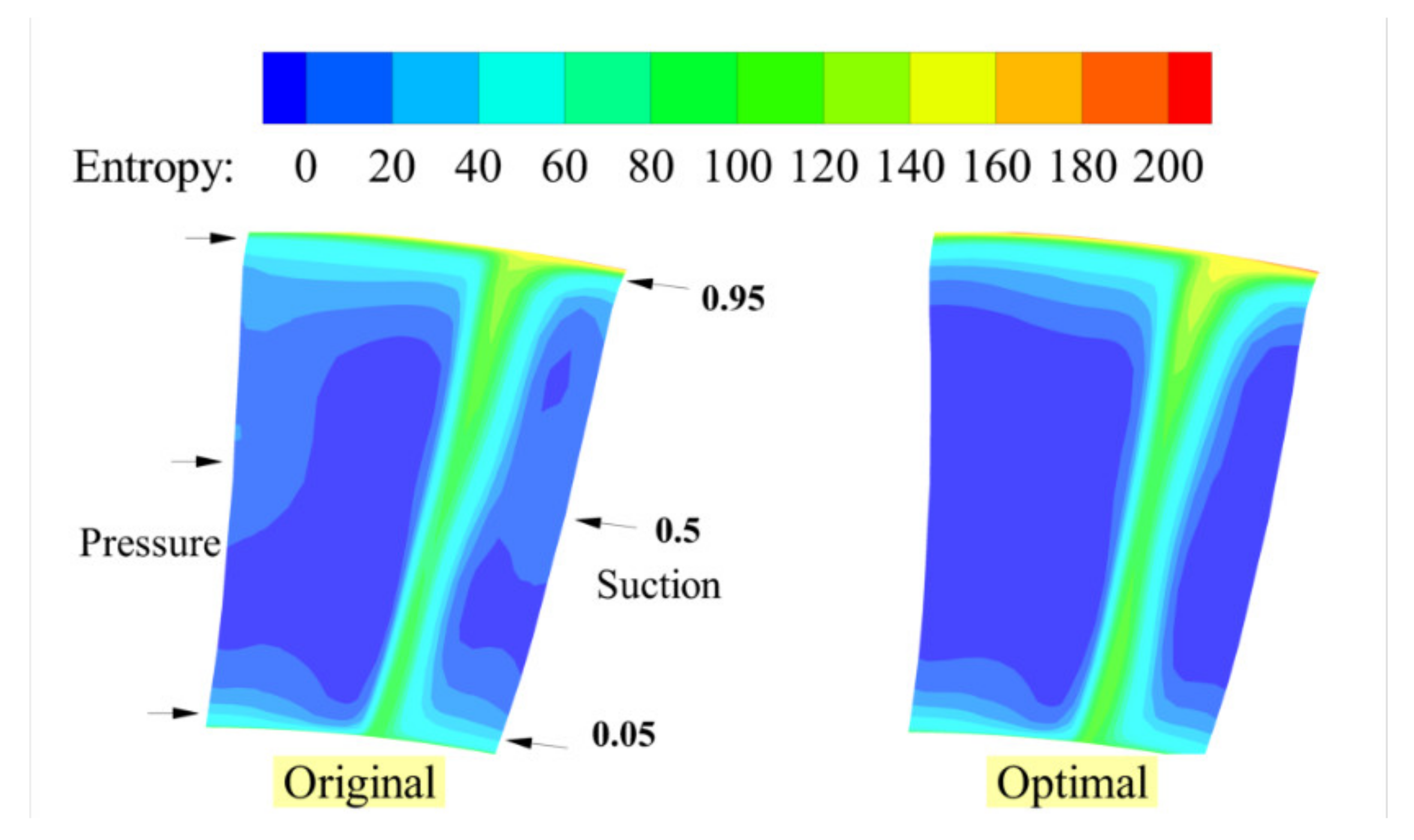
(4) The optimized blade improves the shock wave structure of the flow field, reduces the shock wave intensity at design speed and off-design speed. Additionally, it makes the separation area at the trailing edge of the blade narrow, the suction surface separation line shorten, as well as the blade tip leakage vortex dispersion angle and rotation intensity decrease, thus enhancing the efficiency of the optimized blade.

Although the full-blade surface parametric method has several above advantages, the following defects still exist: it currently does not possess the ability to conduct a sweeping deformation, which limits the geometric exploration ability on the blade in the optimization process to a certain extent. At the same time, the method can make the blade thinner during the geometric changes, and the strength of the rotor blade will be influenced, and need to be more constrained. This parametric method may be more suitable for turbine blades with larger thicknesses. In light of the above problems, further research can be conducted.