Heat Transfer and Hydrodynamics in Stirred Tanks with Liquid-Solid Flow Studied by CFD–DEM Method

Abstract

The heat transfer and hydrodynamics of particle flows in stirred tanks are investigated numerically in this paper by using a coupled CFD–DEM method combined with a standard k-e turbulence model. Particle–fluid and particle–particle interactions, and heat transfer processes are considered in this model. The numerical method is validated by comparing the calculated results of our model to experimental results of the thermal convection of gas-particle flows in a fluidized bed published in the literature. This coupling model of computational fluid dynamics and discrete element (CFD–DEM) method, which could calculate the particle behaviors and individual particle temperature clearly, has been applied for the first time to the study of liquid-solid flows in stirred tanks with convective heat transfers. This paper reports the effect of particles on the temperature field in stirred tanks. The effects on the multiphase flow convective heat transfer of stirred tanks without and with baffles as well as various heights from the bottom are investigated. Temperature range of the multiphase flow is from 340 K to 350 K. The height of the blade is varied from about one-sixth to one-third of the overall height of the stirred tank. The numerical results show that decreasing the blade height and equipping baffles could enhance the heat transfer of the stirred tank. The calculated temperature field that takes into account the effects of particles are more instructive for the actual processes involving solid phases. This paper provides an effective method and is helpful for readers who have interests in the multiphase flows involving heat transfers in complex systems.

1. Introduction

Stirred tanks have been widely used in fermentation, emulsification, crystallization, homogeneous/heterogeneous reaction, and other pharmaceutical and chemical processes [1]. Many of these processes involve liquid–solid multiphase flows and heat transfers. Thus, among stirred reactors, the ones with jackets or coils are the commonest [2]. The study of heat transfers within the stirred reactors is very important since they are crucial in many relevant operations. For example, they are critical to achieve the desired reaction products and prevent the thermal lose control of reactions, as well as to generate the appropriate supersaturation for the product of promising crystals [3].

Experiments and simulations have been employed to study the multiphase flows involving heat transfer [4,5,6,7,8]. However, in many cases, due to different limitations, it is difficult to conduct experiments. Hence, developing numerical method to investigate the heat and mass transfer of multiphase flows in various stirred tanks is of high significance.

Up to now, computational fluid dynamics (CFD) has proved to be an effective tool in the investigation of complex liquid–solid flows involving multi-physical fields. There are a lot of numerical studies of the heat transfer of single-phase flows in stirred tanks. Early research works mainly involved the simulation of heat transfers in mixers with different configurations such as the rounded-bottom vessel with an atypical helical ribbon impeller [9] and the stirred tanks with improved Intermig impellers [10]. Other researchers have focused on the heat transfer characteristics of different fluids in stirred tanks and in a jacketed stirred heat exchanger [3,11,12,13,14,15]. Johnson et al. [15] derived a non-adiabatic heat-transfer model for the study of heat transfers in laboratory to pilot-scale reactors, which could be used to predict the temperature distribution within the uncertainty of the experimental measurements. Although the above works have done a lot on the numerical study of heat transfers of single-phase flows in stirred reactors, there are still few numerical works on the heat transfer of liquid-solid flows in stirred tanks. As many chemical processes in stirred tanks, such as the crystallization, involve heat transfers in multiphase flows containing particles, and as the ignorance of the fluid–particle interaction might result in bigger errors of the numerical results, this paper will try to fill the gap.

The numerical methods modeling particle flows include Eulerian–Eulerian [16,17], Eulerian–Lagrangian [18,19,20], and direct numerical simulations (DNS) [21]. As a Lagrangian method, the discrete phase model (DPM) treats the particles as the mass points and does not consider the volume effects of particles. It is also limited due to its solid volume fraction is generally less than about 10% [22]. The discrete element model (DEM) is popular for calculating the interactions of solid particles with almost real properties and provides several contact models to describe particle collisions. However, it cannot solve the flow problems. Thus, the coupling model of computational fluid dynamics and discrete element model (CFD–DEM) has been widely accepted to calculate the problems of particle flows. As early as 1993, the CFD–DEM model using the coarse-grid approximation, had been developed to study the movement of single particle in fluidized beds [23].

Currently, the CFD–DEM method has been employed to investigate the heat transfer in different processes involving multiphase flow, especially for the gas–solid fluidized beds [24,25,26,27,28,29]. Patil et al. [24] adopted an Euler–Lagrange method to study heat transfers in a fluidized bed and the numerical results are in good agreement to those of the experiments. CFD–DEM method has also been used to study the heat transfer in an aggregate drum dryer to produce hot mix asphalt [26]. The results indicate that the coupled model captures the dominant mode of heat transfers correctly as the particles pass through the hot gases. Recently, a new coupled particle–wall heat transfer algorithm for solving particle–wall heat transfer problems has been proposed by Oschmann et al. [28], and the numerical results are in good agreement to experimental results.

Although many researchers have used CFD–DEM to calculate heat transfers, there are few studies on the mixing process of liquid–solid two-phase flows involving heat transfers. In our previous work, a coupled VOF-DEM model was developed to capture the free surface in gas-liquid-solid systems [22,30,31]. Although they consider the collision among particles and the effects of the particle volume on the continuous phase, no heat transfer has been involved. In this work, CFD–DEM coupling model is extended to investigate particulate flows with both momentum exchange and thermal convection. The calculated temperature fields in stirred tanks involving the liquid-solid flow and the single-phase flow are compared to investigate the influence of particles on the temperature distribution. In addition, by changing the blade height and adding baffles, the influences of these structure parameters on the heat transfer and temperature distribution of the multiphase flow are studied. According to our best knowledge, it is the first work studying the heat transfer of liquid-solid two-phase flows in stirred tanks by using CFD–DEM coupling method. At first, the relevant background and papers are reviewed in the introduction. Then, the mathematical model is described in Section 2. In the third section, the numerical model is verified and validated by several examples. The calculation results are presented and discussed in Section 4. Finally, the conclusions are summarized in Section 5.

2. Model Description

2.1. Fluid Phase

2.1.1. Momentum Equations and Turbulence Model

In the multiphase system, the fluid is considered as a continuous phase and its motion is solved by the continuity equation and momentum equations throughout the domain. The two phases share the velocity field which is based on the local average variable on the mesh cells. Due to the contribution of particles, the continuity and momentum equations can be extended as follows [32]:

$$\frac{\partial ({\rho }_f{\epsilon }_f\mathit{u})}{\partial t}+\nabla \cdot ({\rho }_f{\epsilon }_f\mathit{u}\mathit{u})={\epsilon }_f(-\nabla p+\nabla \cdot (\mathit{\tau }-\rho \overline{{{\mathit{u}}^{\prime }}_i{{\mathit{u}}^{\prime }}_j})+{\mathit{f}}_s+{\rho }_f\mathit{g})+{\mathit{f}}_{pf},$$

(1)

$$\frac{\partial {\epsilon }_f}{\partial t}+\nabla \cdot ({\epsilon }_f\mathit{u})=0,$$

(2)

where ρ_f is fluid density, ԑ_f is the volume fraction of fluid in one cell or the local porosity, following the assumption of local average and u is fluid velocity. Each item on the right side of Equation (1) represents the pressure gradient, stress, gravity and particle–fluid interaction force, respectively.

In this work, the standard k-ԑ model is used to describe the flow since it exhibits better suitability for heat transfer simulations [33].

2.1.2. Energy Equation

Temperature evolution is of great importance in thermal particulate flows. The energy equation is:

$$\frac{\partial ({\rho }_{f}E)}{\partial t}+\nabla \cdot (\mathit{v}({\rho }_{f}E+p))=\nabla \cdot \left(k_{eff}\nabla T-{\displaystyle \sum _j{h}_j{\mathit{J}}_j+({\overline{\mathit{\tau }}}_{eff}\cdot \mathit{v})}\right)+S_h,$$

(3)

where k_eff is the effective thermal conductivity (k_eff = k + k_t, where k_t is the turbulent thermal conductivity, defined according to the used turbulence model.), and J_j is the diffusion flux of species j. The total energy and pressure of fluid are represented by E and p, respectively. The first three terms on the right-hand side of Equation (3) represent the energy transfers due to conduction, species diffusion, and viscous dissipation, respectively. S_h includes the heat of chemical reaction, and any other volumetric heat sources defined by users.

2.2. DEM Model

In the CFD–DEM coupling method, particles are treated as the discrete phase. To track the trajectory of individual particle, its motion is calculated by Newton’s second law. Meanwhile, the rotational momentum of individual particle is solved by the angular momentum equation [19,34]:

$$m_i\frac{d{\mathit{v}}_i}{dt}=-V_i\nabla P+m_i\mathit{g}+{\mathit{F}}_{pf,i}+{\displaystyle \sum _j{\mathit{F}}_{c,ij}},$$

(4)

$$I_i\frac{d{\mathit{\omega }}_i}{dt}={\displaystyle \sum _j{\mathit{T}}_{ij}}$$

(5)

where P is the fluid-phase pressure, V_i is the particle volume, g is the acceleration due to gravity, F_pf,i is the particle-fluid interaction force, and F_c,ij is the contact force, including normal contact force and tangential contact force. m_i, v_i, I_i, ω_i are the mass, the linear velocity, the moment of inertia, and angular velocity of particle i, respectively, T_ij is the torque arising from the tangential and rolling component.

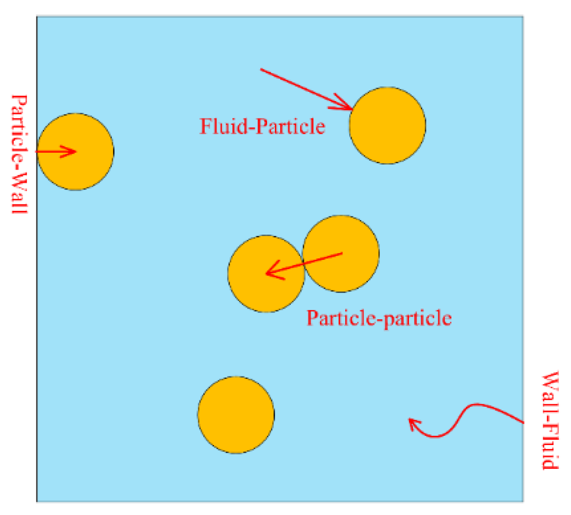
2.3. Interactions in the Multiphase Flow

In this section, the force models and heat transfer models for particles are described, during which the momentum exchange and hear transfer between fluid and particles are presented as well.

2.3.1. Interaction between Particles

Because there are a lot of particles, it is important to calculate the particle–particle and particle–wall interactions which are similar. In this work, the Hertz–Mindlin model is adopted. Based on this, the contact force between two adjacent spherical particles can be divided in to two types: normal contact force [35,36] and tangential force [37], which given as follows. The normal contact force is expressed as:

$${\mathit{F}}_{n,ij}=-k_{n,ij}{\mathit{\delta }}_{n,ij}-{\eta }_{n,ij}{\mathit{v}}_{n,ij},$$

(6)

and the tangential friction force is defined as:

$${\mathit{F}}_{t,ij}=\{\begin{array}{cc}-k_{t,ij}{\mathit{\delta }}_{t,ij}-{\eta }_{t,ij}{\mathit{v}}_{t,ij}& \left(|{\mathit{F}}_{t,ij}|\le {\mu }^{}|{\mathit{F}}_{n,ij}|\right)\\ -{\mu }^{}|{\mathit{F}}_{n,ij}|\frac{{\mathit{v}}_{t,ij}}{|{\mathit{v}}_{t,ij}|}& \left(|{\mathit{F}}_{t,ij}|>{\mu }^{}|{\mathit{F}}_{n,ij}|\right)\end{array},$$

(7)

where k, δ, η and μ are the spring constant, overlap between particles, damping coefficient and friction coefficient, respectively. The subscripts n and t indicate the normal direction, the tangential direction between particles i and j.

The torques generated by the forces can be written as:

$${\mathit{T}}_{t,ij}=L_{ij}{\mathit{n}}_{ij}\times {\mathit{F}}_{t,ij},$$

(8)

$${\mathit{T}}_{r,ij}=-{\mu }_r{L}_{ij}\left|{\mathit{F}}_{n,ij}\right|\frac{{\mathit{\omega }}_{ij}}{\left|{\mathit{\omega }}_{ij}\right|},$$

(9)

where L represents the distance between particles, and subscripts t and r represent tangential and rotational directions, respectively.

2.3.2. Interaction between Particles and Fluid

In this coupling model, the force between fluid and particles have also been taken into accounts, includes the total of drag force, pressure gradient, stresses, Saffman lift force, Magnus lift force. The interaction force is calculated as:

$${\mathit{F}}_{pf,i}={\mathit{F}}_{d,i}+{\mathit{F}}_{\nabla p,i}+{\mathit{F}}_{\nabla \cdot \tau ,i}+{\mathit{F}}_{\nabla \cdot ({\rho }_f{u}_i^{\prime }{u}_j^{\prime }),i}+{\mathit{F}}_{Saff,i}+{\mathit{F}}_{Mag,i}+{\mathit{F}}_{s,i},$$

(10)

The total force per volume:

$${\mathit{f}}_{p,f}=\frac{1}{V_{cell}}{\displaystyle \sum _{i=1}^{n_p}{\mathit{F}}_{pf,i}}-{\mathit{F}}_{\nabla p,i}-{\mathit{F}}_{\nabla \cdot \tau ,i}-{\mathit{F}}_{\nabla \cdot ({\rho }_f{u}_i^{\prime }{u}_j^{\prime }),i}-{\mathit{F}}_{s,i},$$

(11)

The drag force model exerting on the particle is expressed as:

$${\mathit{F}}_d=\frac{\beta V_p}{{\epsilon }_f}(\mathit{u}-\mathit{v}),$$

(12)

where the coefficient β proposed by Ergun and Wen and Yu [38].

The Saffman lift force is calculated by [22]

$${\mathit{F}}_{Saff}=1.61d_p^2{({\mu }_f{\rho }_f)}^{1/2}(\mathit{u}-\mathit{v})\cdot (\nabla \cdot \mathit{u}),$$

(13)

$$\{\begin{array}{ll}\frac{{\mathit{F}}_{L,mei}}{{\mathit{F}}_{Saff}}=(1-0.3314{\alpha }^{1/2})exp\left[-\frac{\mathrm{Re}}{10}\right]+0.3314{\alpha }^{1/2}& \mathrm{Re} \le 40\\ \frac{{\mathit{F}}_{L,mei}}{{\mathit{F}}_{Saff}}=0.0524{(\alpha \mathrm{Re})}^{1/2}& \mathrm{Re} > 40\end{array},$$

(14)

where α = 1/2Re·ԑ² and it ranges from 0.005 to 0.4.

The Magnus lift force is calculated by [22]:

$$\{\begin{array}{l}{\mathit{F}}_{M\mathrm{ag}}=0.125\pi d_p^3{\rho }_f\frac{\mathrm{Re}}{{\mathrm{Re}}_{\mathsf{\Omega }}}{C}_L(0.5{\omega }_c-{\omega }_p)(\mathit{u}-\mathit{v})\\ C_L=0.45+[\frac{{\mathrm{Re}}_{\mathsf{\Omega }}}{\mathrm{Re}}-0.45]\exp (-0.05684{\mathrm{Re}}_{\mathsf{\Omega }}^{0.4}{\mathrm{Re}}^{0.3})\end{array},$$

(15)

when the article rotation is equal to the location rotation of the fluid, the lift force is almost zero.

2.3.3. Particle Heat Transfer

In this work, the heat transfer between particle–particle and particle–fluid are considered. Figure 1 shows the heat exchange mechanisms in a fluid-solid system. In order to evaluate temperature of phases in a coupled CFD–DEM simulation, the energy balance equation for each phase should be added. In the DEM model, a simple method to simulate the heat transfer is provided [34]. The heat flux is expressed as:

$$Q_{ij}=h_c\Delta T_{ij}.$$

(16)

Here, the contact area is incorporated into the heat transfer coefficient h_c

$$h_c=\frac{4k_i{k}_j}{k_i+k_j}{\left(\frac{3F_{n,ij}{r}^{\ast }}{4E^{\ast }}\right)}^{\frac{1}{3}},$$

(17)

where k is thermal conductivity, F_n,ij is the normal contact force, r* is the average radius of particles. After the heat flux is calculated, the temperature of each particle will be updated as [34]:

$$m_p{C}_p\frac{dT}{dt}=\sum Q_{heat},$$

(18)

where m_p, C_p and T are the mass, specific heat capacity and temperature of particles, respectively.

In addition, the convective heat transfer is happened between fluid and particles, which is impelled by the relative motion and temperature difference. Heat transfer flux can be expressed as:

$$Q_{pf}=h_{pf}{A}_p\Delta T_{pf},$$

(19)

where h_pf is the heat transfer coefficient between the two phases, A_p is the surface area of particles and T_pf is the temperature difference between two phases. The heat transfer coefficient is defined as:

$$h_{pf}=\frac{{\kappa }_{q}N{u}_p}{d_p},$$

(20)

where κ_q is the heat conductivity of fluid and the Nussel number Nu_p is a dimensionless number.

2.4. Coupling Scheme

The coupling method used in this work can be divided into three parts, which is presented in Figure 2. Firstly, CFD method initializes the fluid field and trigger the process, then UDF is called to calculate the local porosities and interaction forces. In DEM, the velocity and position of particles are updated by solving motion equation. This information is transmitted to CFD method, and it solves Equations (1)–(3) to update the fluid field and heat field until the process converges. Finally, the fluid field and heat field information return to the DEM. The calculation cycles until the number of steps reaches the set value.

3. Validation and Simulation Setup

In this section, the model and parameter setting in the calculation are first presented, and then, it is validated through the comparison between the calculation results of our model and the experimental data from other literature for the two-phase flows in a gas–solid fluidized bed. Finally, the grid independence is verified.

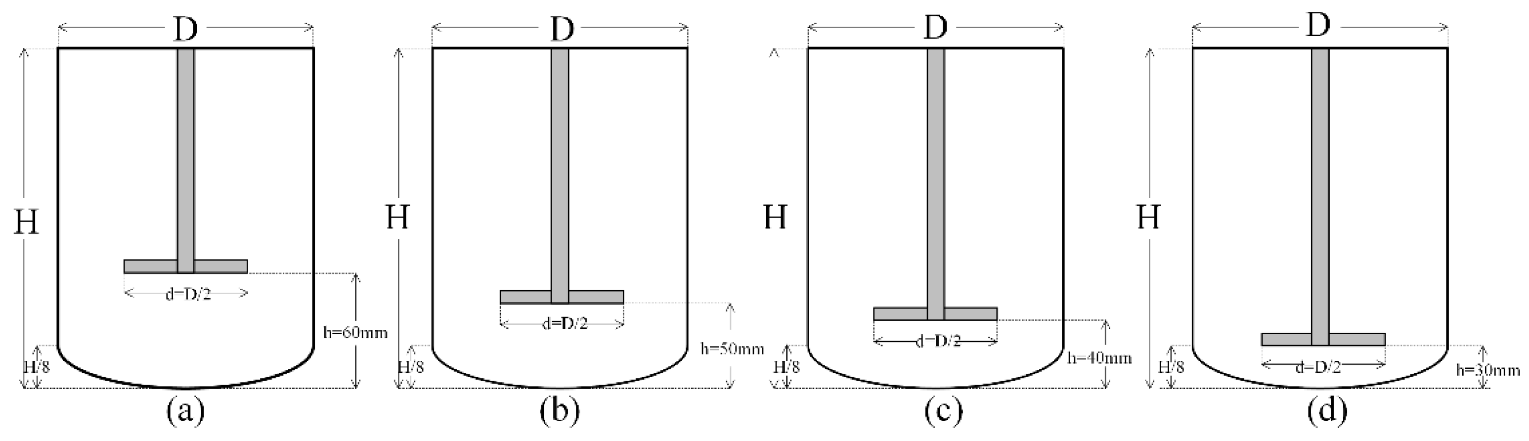
3.1. Configuration of Stirred Tank

In this work, the elliptical bottom tanks with blades of different heights (h) were employed to study the heat transfer, flow patterns, and particle suspension behaviors in the stirred tank. For all of them, the diameter (D) of the tank is 0.15 m and the height (H) is 0.2 m. Four up-pumping stirred blades are 45° pitched and the diameter (d) of the impeller is D/2. Other sizes of these four tanks are shown in Figure 3. At the same time, baffles of 2 mm thickness are equipped in order to explore the influence of them.

3.2. Simulation Details

To simulate impeller rotating, the sliding-grid (SG) algorithm [39] and multiple reference frames (MRF) techniques [16,40] can be used. Since MRF is usually used in the steady-state, the sliding-grid (SG) algorithm is employed in this paper for the calculation of the unsteady-state [41].

In this paper, the liquid phase is water. The physical parameters of water and particles are summarized in

Table 1. Physical properties and model parameters.

Parameter	Value
Water density (kg/m3)	1000
Water viscosity (kg/m∙s)	0.001
Water heat capacity (J/kg∙K)	4182
Water thermal conductivity (W/m∙K)	0.6
Particle density (kg/m3)	1200
Particle heat capacity (J/kg∙K)	1000
Particle thermal conductivity (W/m∙K)	20
CFD time step (s)	5 × 10−4
DEM time step (s)	5 × 10−5
Coupling time step (s)	5 × 10−4
Convergence criteria	1 × 10−5

. The non-slip condition is applied to all the geometry walls, and other properties of the wall and particles are listed in

Table 2. Property of particles and wall in DEM.

Parameter	Particle	Wall	Particle–Particle	Particle–Wall
Particle poisson’s ratio	0.25	0.3	-	-
Particle shear modulus/MPa	1	7 × 104 Pa	-	-
Coefficient of restitution	-	-	0.3	0.2
Coefficient of static friction	-	-	0.5	0.5
Coefficient of rolling friction	-	-	0.01	0.01

. Meanwhile, in order to calculate the cooling process in stirred tanks, initial temperature of the particles and water is set at 350 K, and boundary conditions of the side and bottom surfaces of the stirred tank are set to convection where the free stream is at 280 K. In practice, the cool water in jacket of the stirred tanks enters from the bottom, thus the external convection heat transfer coefficient on the bottom surface is set to be greater than that on the wall surface, which is 4200 W/(m²·K) and 3000 W/(m²·K), respectively.

3.3. CFD–DEM Model and Experimental Verification

To verify whether this CFD–DEM model is suitable for heat and momentum transfers, our numerical results are compared to the experiment data of Patil et al. [24].

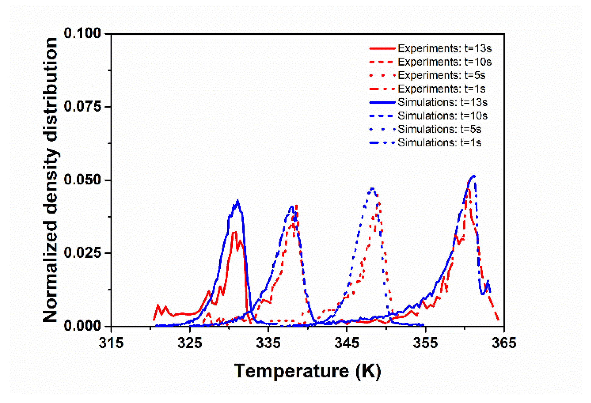
3.3.1. Heat Model and Flow Pattern Validation

In order to validate the CFD–DEM model involving heat transfers, two-phase flows with heat transfers in a gas–solid fluidized bed are calculated according to the same conditions as those in paper by Patil et al. [24]. In their works, the size of the fluidized bed is 1.5 × 8 × 25 cm³, and the initial temperatures of the particle bed and injected gas are 263.15 K and 293.15 K, respectively. Around the inlet center, there is a nozzle cover sealing the hot gas inlet, which is not used in the present experiment, as shown in Figure 4.

For the CFD–DEM simulation, the mesh number is set to be 6 × 32 × 100. The velocity boundary condition on the nozzle cover is set to no-slip. Other details of this simulation are summarized in

Table 3. Properties and settings used in the simulation.

Parameter	Value
Particle density (kg/m3)	2500
Fluid heat capacity (J/kg∙K)	1010
Fluid thermal conductivity (W/m∙K)	0.0242
Particle heat capacity (J/kg∙K)	840
Particle thermal conductivity (W/m∙K)	1.4
Fluid viscosity (kg/m∙s)	2 × 10−5

.

According to these settings, the CFD–DEM method is validated by comparing the temperature density distribution (TDD) of particles and the average temperature of the powder bed. Firstly, Figure 5 shows a series of snapshots of the fluidized bed at different time t = 2 s, t = 4 s and t = 12 s, and both the flow patterns and temperature distributions are similar to the infrared images recorded by Patil et al. [24].

In order to analyze the fluidized bed with thermal convection, the distribution of the particle temperature provides information that is of great concern. The temperature density distribution is a good parameter to present the distribution clearly, which is the quantitative description about the temperature of most particles and the temperature range of the fluidized bed. As shown in Figure 6, the overall profiles of TDD are quite consistent to the experimental results, especially when time is 1 s and 10 s.

Another important measure of the model accuracy is the average temperature of the fluidized bed. Figure 7 shows the comparison of the calculated results to those experimental data of the mean temperature. The maximum relative error between the numerical and experimental results is less than 1%, which means that the results of the CFD–DEM model are consistent to those of the experiments. Thus, in the following sections, this coupled CFD–DEM method will be employed to calculate the convective heat transfer of liquid-solid flows in stirred tanks.

3.3.2. Grid Independence Verification

The purpose of this work is to study the particulate flows with heat transfer in the stirred tanks. The selection of grid sizes is critical to the calculation process of CFD: coarse grids might result in a poor calculation accuracy, while fine grids will increase the computation costs. In this paper, the computation domains are divided into the dynamic region and the static region. As for them, the dynamic region uses a finer mesh, while the static region is discretized into relatively coarse grids.

In order to choose an appropriate grid size, five combinations of grid sizes are designed: 2 mm + 6 mm, 3 mm + 7 mm, 4 mm + 8 mm, 5 mm + 9 mm, 6 mm + 10 mm. The 2 mm + 6 mm combination represents that 2 mm meshes are employed in the dynamic region and 6 mm meshes are used in the static region. The total grid numbers are 407,167, 328,877, 296,340, 254,028 and 233,225, respectively. To compare the accuracy of the calculation results of different grid sizes, it is assumed that the results of the smallest grid combination (2 mm + 6 mm) are the actual results. The mean temperature of the stirred tank is chosen to do the grid independence verification.

Figure 8 shows the relative errors of the calculated results of five grid combinations when time is 1 s. As the number of grids increases, the relative error δ decreases rapidly firstly, but after the number of 254,028, the change becomes very limited. Since the relative error is less than 0.1% when the grid number is 296,340, it means that the accuracy is high enough and there is no need to reduce the grid size further. Thus, the mesh size of 4 + 8 mm is adopted in this paper.

4. Results and Discussion

In this section, the heat transfer in stirred tanks with and without particles is first compared. Then, the effects of blade heights and baffles on the heat transfer and hydrodynamics of the liquid-solid flow in stirred tanks are investigated. Four heights of blades from the bottom (30 mm, 40 mm, 50 mm and 60 mm) are considered. The diameter of particles is 1.5 mm, the number of particles is 50,000 and the agitator speed is 600 rpm. At time t = 0 s, particles are accumulated on the bottom of stirred tanks.

4.1. Effects of Particles on Heat Transfer

In Figure 9a,b, the temperature distributions on XZ plane in the tank with and without particles are compared. It is obvious that the temperature fields are different for the two tanks due to the effects of the particles. Firstly, although there is a low temperature zone just below the stirrer for both cases, the sizes of the zone are different. For the tank with single-phase flow, this zone is narrow and the temperature adjacent to the blade is a little higher (see Figure 9a); for the tank with particle flows, this zone is wider, and the temperature is relatively lower (see Figure 9b), which might be because of the particle accumulation in the dead zone below the stirrer. In addition, the former has a greater temperature gradient near the wall of the middle tank than the latter, and for the latter, the low temperature green zone is relatively wider. This is because for the former, the water boundary layer decreases the heat transfer rate, and for the latter, the zone near the wall surface is occupied by particles and the heat transfer boundary layer is obviously weakened due to the collision of the particles which are relatively easier to conduct heat. The particle distribution could be seen clearly in next sections (Figure 10a). At the top part of the tank with the single-phase flow, there is a low temperature zone like the elephant nose, while, for the tank with particle flows, there is no such a zone. When there are no particles in the tank, the heat transfer inside the tank is dominated by the flow circulation. The low temperature belt zones just follow the currents whose direction is from the wall to central zone of the tank. However, when there are a lot of particles in the tank, the chaotic movement and collision of particles might enhance the turbulence of the flow and change the circulation, and further change the heat transfer inside the tank. Figure 9c is amplified figure of region B picked from Figure 9b, which shows the fluid and particle temperature in this zone on XZ plane of the stirred tank with particle flows. It can be seen that there is a little difference between temperature of particles and surrounding fluid and temperature of most particles near the bottom is lower than the surrounding fluid. At time t = 0, all the particles are closely settled at the bottom, and at t = 1 s, most of these particles are still at the bottom, especially for those in the dead zone. Thus, for those particles, the heat conduction between particles is strong. At the meantime, the hot fluid from the center of the tank and the cold fluid near the bottom mix more quickly than the upward movement of the cooler particles near the bottom under the stirring action. Thus, it is reasonable that the temperature of particles near the bottom is relatively lower than the surrounding fluid. When the calculation reaches 5 s, the average temperature of the fluid in the stirred tank for the single-phase flow and particle flow is 345.389 K and 343.55 K, respectively. It can be seen that the existence of particles enhances the heat transfer in the stirred tank.

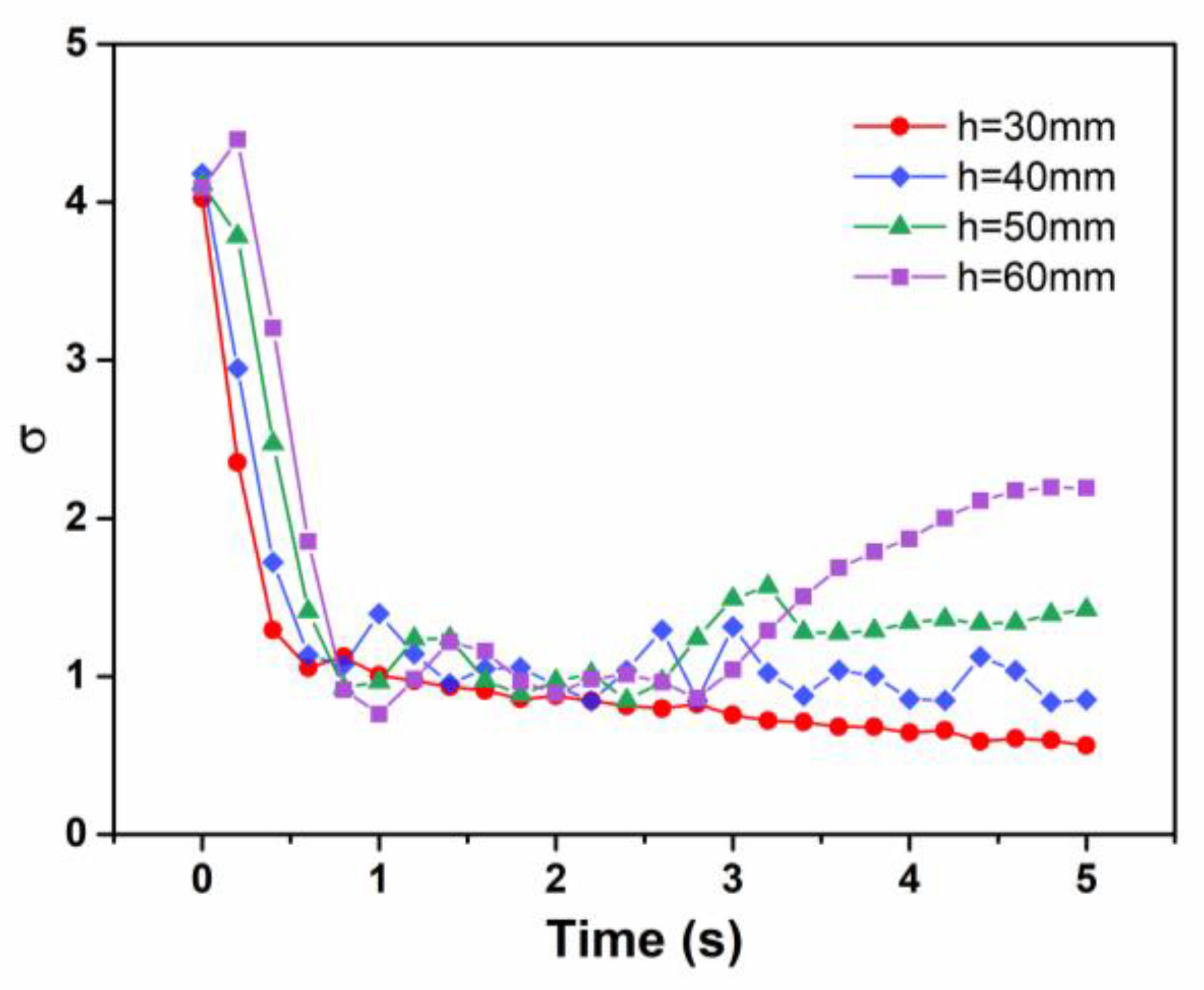
4.2. Effects of Blade Height on Heat Transfer and Hydrodynamic

The snapshots of temperature and distribution of particles in four tanks are displayed in Figure 10. In order to clearly see the particle temperature range, a different range is used for each moment of the legend in Figure 10. It can see that particles are inhaled upward by the rotation of blades at the beginning of the agitation, and subsequently thrown off by the stirrer and move toward the wall along with the radial flow. When touching the wall, particles move along the wall with the upward and downward axial flow. It can be seen that the higher the blade is, the higher the particles could reach along with the upward axial flow (see Figure 10, t = 1 s). However, the particles cannot reach the top of the stirred tank when h = 30 mm. Then, the fluid will form a loop in each of the upper and lower sections of blades due to the negative pressure caused by the blade rotation. When the mixing processes reach the stable state, a strong tangential flow is formed in the tanks, which results in the accumulation of particles in the conical dead zone below the blades and in the upper circular belt zone (see Figure 10, t = 5 s). With the increase of the blade height, the negative pressure zone at the bottom is enlarged, causing more particles to remain in the dead zone. The upper particles form a narrower and sparser but higher ring since the number of rising particles gets less. For h = 30 mm, more than half of all the particles can be suspended above the blades. Moreover, in the steady state, the upper particles in this case do not form the circular belt and could rise almost to the same height as those in other cases. In contrast, only 7% of the particles are suspended over blades for h = 60 mm. It can be asserted that reducing the blade height is beneficial to the mixing process.

To describe the homogeneity degree of particles in stirred tanks, the variation coefficient σ is used to qualify the suspension of particles, which is defined by Equation (21) [42,43].

$$\sigma =\sqrt{\frac{1}{\mathrm{n}}{{\displaystyle \sum _{i=1}^n\left(\frac{{\alpha }_{2i}}{{\alpha }_{2,av}}-1\right)}}^2},$$

(21)

where α_2i is the particle volume fraction in each part, α_2,av is the average of particle volume fractions in all parts. In this work, the whole domain covered by water is divided into 36 cells, thus the value of n in this formula is 36. Figure 11 shows the value variation of σ over time for four cases. In all the four stirred tanks, σ firstly decreases and finally fluctuates around a certain value. It can be seen that the homogeneity degree of particles decreases with the increase of blade heights at the final stage of mixing. The results here are similar to those of Blais et al. [44].

In order to understand the hydrodynamics in the stirred tanks, the velocity vectors on XZ plane of the stirred tanks at t = 5 s are shown in Figure 12. It is obvious that the lower loop is expanded as the blades are elevated. In the conical dead zone and the upper circular belt zone, the axial and radial velocities are very weak. As the blade height increases, the axial velocity of the fluid near the bottom decreases, resulting in the expansion of the negative pressure zone, and more particles are trapped in the dead zone. As a result, the homogeneity degree of particles decreases.

The temperature distribution of particles can also be clearly seen in Figure 10. It shows that temperature of particles in stirred tanks can be divided into several parts. Firstly, particles on the bottom of the tanks have the lowest temperature of all particles. Because the axial velocities near the bottom are relatively low, most particles near the bottom stay on the bottom surface for a longer time, and thus, their temperature is low. Subsequently, in the process of being inhaled, the particles are far away from the convective wall and mixed with hot fluid inside the tank, resulting in the decrease of heat transfer rate. As mentioned before, the radial and axial flows which contributes to the convective heat transfer efficiency of the stirred tanks in the dead zone are weak, resulting in a lower rate of heat transfer. Thus, particles which are just thrown off by blades have the highest temperature of all, which becomes more pronounced as the blades rise (Figure 10, t = 1 s). The powerful radial flow generated by the blades brings the internal hot fluid to the wall and causes the heat transfer between the hot fluid and the cold wall. In the axial movement along the wall, the heat transfer rate of the particles increases, and the temperature drops quickly. After reaching the steady state, the upper particles stay in the circular belt area near the wall due to the strong tangential velocity and gradually cool down. The particles near the blade cool down due to the lower and upper loop of the flow, and finally the entire tank is fully cooled down when the blade height is the lowest (Figure 10a, t = 5 s). For other three cases, the entire tanks could not be fully cooled down when t = 5 s.

The temperature of particles on the bottom can be observed more clearly from the bottom-view diagram (see Figure 13), and the legend is consistent with Figure 10. From Figure 13, it can be seen that the temperature of the bottom particles presents a circular distribution. The temperature of the central particles is low and gradually increases towards the circular boundary. In the initial stage (t = 1 s), due to the different upward speeds of the bottom particles, the higher the blade is, the longer the particles stay at the bottom, and thus, the larger the central low temperature circle zone will be. However, these circular zones disappear as the stirring process develops (t = 5 s). Due to the circulation inside the tanks, the temperature of particles gets uniform gradually along with the time. When the blades height gets down, the fluid shear forces near the tank bottom become much stronger. When h = 30 mm, the dead zone is replaced by a central blank area as the swirling motion dominates particles (Figure 13a). Due to the elimination of the dead zone, more particles are suspended, resulting in the increase of the heat transfer efficiency. At the meantime, the collision between particles is enhanced, which makes the temperature distribution of particles more uniform.

Compared to the traditional CFD methods, the major advantage of our method is that more details of the particle motion and temperature distribution could be calculated and exhibited like in Figure 10 and Figure 13. It is more helpful for researchers to analyze the heat transfer and hydrodynamic behaviors of particles in complex reactors.

As can be seen from both Figure 10 and Figure 13, when the blade height decreases, the particle temperature drops a little faster, and the temperature range of the particles is also narrower. It also could be observed from Figure 14, density distribution curves of the particle temperature. At the initial stage (t = 1 s), particles in four tanks have similar distribution of the temperature, and the temperature range is relatively big, from 346 K to 349 K. It can be seen that there are two peaks in the temperature distribution curves. The first peak (about 349 K) might be caused by the earliest particles which are inhaled by the blade rotation, and the second (about 348.3 K) might be due to the particles staying in the dead zone. As the stirring process goes on, the temperature becomes more and more uniform (Figure 14b,c). However, due to the large dead zone, the particle temperature range is still relatively large when h = 50 mm and h = 60 mm. The peaks of the curves in Figure 14b,c show that the particle cooling is faster when the flow near the bottom is strengthened due to the low height of the blade.

Figure 15 and Figure 16 show the heat flux through the wall and the bottom of the stirred tanks when time is 1 s, respectively. The negative sign in the temperature scale bar indicates that the heat flow is from the inside to the outside of the tanks. As shown in Figure 15, it is clear that there is a circular belt distribution of the heat flux through the wall, and the heat flux reaches the maximum around the horizontal plane of the blades. Compared to Figure 12, the heat flux is higher at the location where the radial flow is stronger. Thus, enhancing the radial flows will be effective to enhance the heat transfer efficiency of the stirred tanks. From Figure 16, a ring distribution of the heat flux could be seen due to the influence of the rotating flow. Obviously, the heat flux becomes more uniform as the blade height decreases. This could be explained by Figure 17, which shows the tangential velocity of the flow at the height H = 0.015 m on YZ plane. The tangential velocity increases as the blade rises, resulting in the enlargement of the dead zones. Compared to other three cases, the dead zone could be eliminated when the blade height is 30 mm, and thus, the particle temperature in the stirred tank will be more uniform and the heat transfer rate is higher.

4.3. Effects of Baffles on Heat Transfer and Hydrodynamic

In the stirring process, baffles are employed to eliminate the tangential flow and to strengthen the axial and radial flow. The stirred tank with the blades height of 30 mm, which has a better result as shown in last section, is selected to add the baffles and studied in this section.

Figure 18 shows the snapshots of the temperature and distribution of particles. The temperature range in the legend is chosen differently from Figure 10, which is to better represent the particle temperature distribution. Comparing to the stirred tanks without baffles (Figure 10a), particles are suspended in the tank more violently. Due to the baffles, the tangential movement of particles are constrained, the axial and radial movement are remarkably enhanced. At the initial stage (t = 1 s), more particles driven by the stirrer moving toward the wall change to the upward and downward movement due to the hindering of baffles. When the system reaches the steady state, particles in the upper zone of the tank could not form a ring belt since the tangential velocity are strongly weakened, and much more particles could reach the top zone of the tank. Figure 19 shows the variation of σ along with time. Compared to the stirred tank without baffles, the values of σ are generally smaller for the tank with baffles. Obviously, the mixing degree of the tank with baffles is higher. The enhanced axial and radial flows strengthen the main body circulation in the tank and drive more particles moving upward and suspending. Figure 20 shows the comparison of the radial velocities of different heights at the location r/R = 2/3 between the tanks with and without baffles. The positive and negative velocities indicate the outward and inward direction of the movement, respectively. At the same height, the axial velocity is greater in the tank with baffles. Moreover, due to the remarkable enhancement of the turbulence of the circulation, the convective heat transfer efficiency is increased significantly. Thus, the cooling rate of the tank with baffles is elevated. When t = 5 s, the average temperature of particles in the tank with baffles is about 1 K less than that in the tank without baffles.

Figure 21 shows the temperature of particles near the bottom of the stirred tanks and the legend is consistent with Figure 18. Similarly, temperature of particles around the center is lower than those near the wall. The difference is that the particles with lower temperature form a spiral shape rather than a circle in the baffled tank. This is because the baffles block the tangential flow, allowing the particles to accumulate behind the baffles, where the particles are cooled down more quickly. When the system reaches the steady state (t = 5 s), because the radius of the rotating flow is reduced, a blank area without particles at the bottom cannot be formed, and the particles with lower temperature appear in a cross-like shape. It could be supported by Figure 22, which shows the comparison of the tangential velocity at H = 0.015 m on YZ plane of the tanks with and without baffles. The tangential velocity decreases significantly beyond 1/2 of the radius in the tank with baffles.

The comparison of density distribution curves of particle temperature in the tanks with and without baffles is shown in Figure 23. It can be seen that the temperature of particles in the tank with baffles drop a little faster. When t = 1 s, the particle temperature distribution is roughly the same. However, when t = 3 s, the average temperature for both two cases are almost the same, but the distribution in the tank with baffles was wider than that in the tank without baffles. When the stirring process reaches the steady state, the temperature in the tank with baffles gets down more than that in the tank without baffles, but its distribution is wider than the latter. This might be because the particles are too dispersed in the tank and there is still a dead zone, resulting in the probability of particle collisions is reduced.

5. Conclusions

In this work, the heat transfer and hydrodynamics in the stirred tanks with liquid-solid flow are studied by using the coupled CFD–DEM model. This model takes into account both the heat transfer between particles and between particles and fluid, which can accurately capture the temperature of a single particle. In order to ensure the accuracy of the model, a series of verification are carried out.

The heat transfer of liquid-solid flows in the stirring process is studied for the first time in this paper. By comparing the heat transfer between the single-phase flow and liquid–solid flow in the stirred tanks, it is disclosed that particles have obvious influences on the heat transfer in stirred tank, which has seldom been studied in the literature. Several stirred tanks, which have blades of different heights or which are equipped with baffles or not, are studied carefully. The numerical results show that, within the range set by this study, the decrease of blade heights has a good effect on the heat transfer and mixing of particles in the stirred tanks. Compared to other cases, the particle temperature is more uniform and drops faster when the blade height is 30 mm (about H/6). In addition, the particles are mixed more evenly. After adding four baffles, the tangential flow in the stirred tank is constrained and the radial and axial flow are enhanced, resulting in the enhancement of the heat transfer efficiency and the degree of mixing. However, the temperature distribution of particles is wider.

The above results show that the radial flow is important for the heat transfer in the stirred tanks with particle flows. In addition, the large dead zone has a negative effect on the uniformity of the particle temperature and the heat transfer efficiency. Thus, the enhancement of the radial flow and the elimination of the dead zone are important to enhance the heat transfer efficiency in the stirred tanks with particle flows.

In general, this coupled method is effective for calculating multi-phase flows involving heat transfers. This work is helpful for readers to understand the influence of particles on the heat transfer of chemical processes in stirred tanks, and the results of the effects of the blade height and baffles on the heat transfer is also useful in the design of the stirred tanks. However, the heat transfer inside the particle and between the particle and wall are not considered. Also, this paper only considers a case in which the thermal conductivity of particles is greater than that of water, and the opposite case would be an interesting research direction. In the future, more comprehensive and deep studies about this topic will be carried out.

References

1. Mahmud, T.; Haque, J.N.; Roberts, K.J.; Rhodes, D.; Wilkinson, D. Measurements and modelling of free-surface turbulent flows induced by a magnetic stirrer in an unbaffled stirred tank reactor. Chem. Eng. Sci. 2009, 64, 4197–4209. [Google Scholar] [CrossRef]
2. Mckeown, R.R.; Wertman, J.T.; Dell’Orco, P.C. Crystallization Design and Scale-Up; John Wiley & Sons, Ltd.: Hoboken, NJ, USA, 2010. [Google Scholar]
3. Bentham, E.J.; Heggs, P.J.; Mahmud, T. CFD modelling of conjugate heat transfer in a pilot-scale unbaffled stirred tank reactor with a plain jacket. Can. J. Chem. Eng. 2019, 97, 573–585. [Google Scholar] [CrossRef]
4. Barnoon, P.; Toghraie, D.; Dehkordi, R.B.; Abed, H. MHD mixed convection and entropy generation in a lid-driven cavity with rotating cylinders filled by a nanofluid using two-phase mixture model. J. Magn. Magn. Mater. 2019, 483, 224–248. [Google Scholar] [CrossRef]
5. Carcadea, E.; Ingham, D.B.; Stefanescu, I.; Ionete, R.; Ene, H. The influence of permeability changes for a 7-serpentine channel pem fuel cell performance. Int. J. Hydrogen Energy 2011, 36, 10376–10383. [Google Scholar] [CrossRef]
6. Gheynani, A.R.; Akbari, O.A.; Zarringhalam, M.; Shabani, G.A.S.; Alnaqi, A.A.; Goodarzi, M.; Toghraie, D. Investigating the effect of nanoparticles diameter on turbulent flow and heat transfer properties of non-Newtonian carboxymethyl cellulose/CuO fluid in a microtube. Int. J. Numer. Methods Heat Fluid Flow 2019, 29, 1699–1723. [Google Scholar] [CrossRef]
7. Toghraie, D.; Karami, A.; Afrand, M.; Karimipour, A. Effects of geometric parameters on the performance of solar chimney power plants. Energy 2018, 162, 1052–1061. [Google Scholar] [CrossRef]
8. Toghraie, D.; Mahmoudi, M.; Akbari, O.A.; Pourfattah, F.; Heydari, M. The effect of using water/CuO nanofluid and L-shaped porous ribs on the performance evaluation criterion of microchannels. J. Therm. Anal. Calorim. 2019, 135, 145–159. [Google Scholar] [CrossRef]
9. Delaplace, G.; Torrez, C.; Leuliet, J.C.; Belaubre, N.; Andre, C. Experimental and CFD Simulation of Heat Transfer to Highly Viscous Fluids in an Agitated Vessel Equipped With a non Standard Helical Ribbon Impeller. Chem. Eng. Res. Des. 2001, 79, 927–937. [Google Scholar] [CrossRef]
10. Wang, L.Z.; Zhou, Y.J.; Chen, Z.B. Investigation of Heat Transfer Efficiency of Improved Intermig Impellers in a Stirred Tank Equipped with Vertical Tubes. Int. J. Chem. React. Eng. 2020, 18, 20. [Google Scholar] [CrossRef]
11. Perarasu, T.; Arivazhagan, M.; Sivashanmugam, P. Experimental and CFD Heat Transfer Studies of Al2O3- Water Nanofluid in a Coiled Agitated Vessel Equipped with Propeller. Chin. J. Chem. Eng. 2013, 21, 1232–1243. [Google Scholar] [CrossRef]
12. Hafezisefat, P.; Esfahany, M.N.; Jafari, M. An experimental and numerical study of heat transfer in jacketed vessels by SiO2 nanofluid. Heat Mass Transf. 2017, 53, 2395–2405. [Google Scholar] [CrossRef]
13. Sivashanmugam, P. Numerical studies on heat transfer characteristics of graphite-water microfluid in a coiled agitated vessel. Heat Transf. Asian Res. 2018, 47, 824–834. [Google Scholar] [CrossRef]
14. Jayakumar, J.S.; Mahajani, S.M.; Mandal, J.C.; Vijayan, P.K.; Bhoi, R. Experimental and CFD estimation of heat transfer in helically coiled heat exchangers. Chem. Eng. Res. Des. 2008, 86, 221–232. [Google Scholar] [CrossRef]
15. Johnson, M.; Al-Dirawi, K.H.; Bentham, E.; Mahmud, T.; Heggs, P.J. A Non-Adiabatic Model for Jacketed Agitated Batch Reactors Experiencing Thermal Losses. Ind. Eng. Chem. Res. 2021, 60, 1316–1325. [Google Scholar] [CrossRef]
16. Hosseini, S.; Patel, D.; Ein-Mozaffari, F.; Mehrvar, M. Study of Solid-Liquid Mixing in Agitated Tanks through Computational Fluid Dynamics Modeling. Ind. Eng. Chem. Res. 2010, 49, 4426–4435. [Google Scholar] [CrossRef]
17. Visuri, O.; Liiri, M.; Alopaeus, V. Comparison and validation of CFD models in liquid–solid suspensions. Can. J. Chem. Eng. 2011, 89, 696–706. [Google Scholar] [CrossRef]
18. Srinivasa, T.; Jayanti, S. An Eulerian/Lagrangian study of solid suspension in stirred tanks. AIChE J. 2007, 53, 2461–2469. [Google Scholar] [CrossRef]
19. Zhu, H.P.; Zhou, Z.Y.; Yang, R.Y.; Yu, A.B. Discrete particle simulation of particulate systems: Theoretical developments. Chem. Eng. Sci. 2007, 62, 3378–3396. [Google Scholar] [CrossRef]
20. Lain, S.; Broder, D.; Sommerfeld, M.; Goz, M.F. Modelling hydrodynamics and turbulence in a bubble column using the Euler-Lagrange procedure. Int. J. Multiph. Flow 2002, 28, 1381–1407. [Google Scholar] [CrossRef]
21. Li, G.H.; Li, Z.P.; Gao, Z.M.; Wang, J.W.; Bao, Y.Y.; Derksen, J.J. Particle image velocimetry experiments and direct numerical simulations of solids suspension in transitional stirred tank flow. Chem. Eng. Sci. 2018, 191, 288–299. [Google Scholar] [CrossRef] [Green Version]
22. Kang, Q.Q.; He, D.P.; Zhao, N.; Feng, X.; Wang, J.T. Hydrodynamics in unbaffled liquid-solid stirred tanks with free surface studied by DEM-VOF method. Chem. Eng. J. 2020, 386, 17. [Google Scholar] [CrossRef]
23. Tsuji, Y.; Kawaguchi, T.; Tanaka, T. Discrete Particle Simulation of 2-Dimensional Fluidized-Bed. Powder Technol. 1993, 77, 79–87. [Google Scholar] [CrossRef]
24. Patil, A.V.; Peters, E.; Kuipers, J.A.M. Comparison of CFD-DEM heat transfer simulations with infrared/visual measurements. Chem. Eng. J. 2015, 277, 388–401. [Google Scholar] [CrossRef]
25. Wang, Z.; Liu, M. Semi-resolved CFD-DEM for thermal particulate flows with applications to fluidized beds. Int. J. Heat Mass Trans. 2020, 159, 120150. [Google Scholar] [CrossRef]
26. Hobbs, A. Simulation of an aggregate dryer using coupled CFD and DEM methods. Int. J. Comput. Fluid Dyn. 2009, 23, 199–207. [Google Scholar] [CrossRef]
27. Sousani, M.; Hobbs, A.M.; Anderson, A.; Wood, R. Accelerated heat transfer simulations using coupled DEM and CFD. Powder Technol. 2019, 357, 367–376. [Google Scholar] [CrossRef]
28. Oschmann, T.; Kruggel-Emden, H. A novel method for the calculation of particle heat conduction and resolved 3D wall heat transfer for the CFD/DEM approach. Powder Technol. 2018, 338, 289–303. [Google Scholar] [CrossRef]
29. Golshan, S.; Sotudeh-Gharebagh, R.; Zarghami, R.; Mostoufi, N.; Blais, B.; Kuipers, J.A.M. Review and implementation of CFD-DEM applied to chemical process systems. Chem. Eng. Sci. 2020, 221, 35. [Google Scholar] [CrossRef]
30. Wu, L.; Gong, M.; Wang, J.T. Development of a DEM-VOF Model for the Turbulent Free-Surface Flows with Particles and Its Application to Stirred Mixing System. Ind. Eng. Chem. Res. 2018, 57, 1714–1725. [Google Scholar] [CrossRef]
31. Zhao, N.; Wang, B.; Kang, Q.Q.; Wang, J.T. Effects of settling particles on the bubble formation in a gas-liquid-solid flow system studied through a coupled numerical method. Phys. Rev. Fluids 2020, 5, 24. [Google Scholar] [CrossRef]
32. Lu, Y.; Huang, J.; Zheng, P. A CFD-DEM study of bubble dynamics in fluidized bed using flood fill method. Chem. Eng. J. 2015, 274, 123–131. [Google Scholar] [CrossRef]
33. Aubin, J.; Fletcher, D.F.; Xuereb, C. Modeling turbulent flow in stirred tanks with CFD: The influence of the modeling approach, turbulence model and numerical scheme. Exp. Therm. Fluid Sci. 2004, 28, 431–445. [Google Scholar] [CrossRef] [Green Version]
34. Zhu, H.P.; Zhou, Z.Y.; Yang, R.Y.; Yu, A.B. Discrete particle simulation of particulate systems: A review of major applications and findings. Chem. Eng. Sci. 2008, 63, 5728–5770. [Google Scholar] [CrossRef]
35. Shigeto, Y.; Sakai, M. Arbitrary-shaped wall boundary modeling based on signed distance functions for granular flow simulations. Chem. Eng. J. 2013, 231, 464–476. [Google Scholar] [CrossRef]
36. Shao, T.; Hu, Y.; Wang, W.; Jin, Y.; Cheng, Y. Simulation of Solid Suspension in a Stirred Tank Using CFD-DEM Coupled Approach. Chin. J. Chem. Eng. 2013, 21, 1069–1081. [Google Scholar] [CrossRef]
37. Ai, J.; Chen, J.F.; Rotter, J.M.; Ooi, J.Y. Assessment of rolling resistance models in discrete element simulations. Powder Technol. 2011, 206, 269–282. [Google Scholar] [CrossRef]
38. Sun, X.; Sakai, M. Three-dimensional simulation of gas-solid-liquid flows using the DEM-VOF method. Chem. Eng. Sci. 2015, 134, 531–548. [Google Scholar] [CrossRef]
39. Micale, G.; Grisafi, F.; Rizzuti, L.; Brucato, A. CFD simulation of particle suspension height in stirred vessels. Chem. Eng. Res. Des. 2004, 82, 1204–1213. [Google Scholar] [CrossRef]
40. Wang, S.Y.; Jiang, X.X.; Wang, R.C.; Wang, X.; Yang, S.W.; Zhao, J.; Liu, Y. Numerical simulation of flow behavior of particles in a liquid-solid stirred vessel with baffles. Adv. Powder Technol. 2017, 28, 1611–1624. [Google Scholar] [CrossRef]
41. Blais, B.; Bertrand, O.; Fradette, L.; Bertrand, F. CFD-DEM simulations of early turbulent solid-liquid mixing: Prediction of suspension curve and just-suspended speed. Chem. Eng. Res. Des. 2017, 123, 388–406. [Google Scholar] [CrossRef]
42. Bohnet, M.; Niesmak, G. Feststoffverteilung in gerührten Suspensionen. Chem. Ing. Tech. 1979, 51, 314–315. [Google Scholar] [CrossRef]
43. Xie, L.; Luo, Z.H. Modeling and simulation of the influences of particle-particle interactions on dense solid-liquid suspensions in stirred vessels. Chem. Eng. Sci. 2018, 176, 439–453. [Google Scholar] [CrossRef]
44. Blais, B.; Bertrand, F. CFD-DEM investigation of viscous solid-liquid mixing: Impact of particle properties and mixer characteristics. Chem. Eng. Res. Des. 2017, 118, 270–285. [Google Scholar] [CrossRef]
Figure 1. Heat exchange mechanisms in a fluid–solid system.
Processes 09 00849 g001
Figure 2. Computing cycle of CFD–DEM model.
Processes 09 00849 g002
Figure 3. Configurations of the stirred tank with the height of blades is (a) 30 mm. (b) 40 mm. (c) 50 mm. (d) 60 mm.
Processes 09 00849 g003
Figure 4. Structure diagram of pneumatic fluidized bed.
Processes 09 00849 g004
Figure 5. Schematic diagram of particle behaviors and temperature distribution when time is (a) 2 s, (b) 4 s and (c) 12 s.
Processes 09 00849 g005
Figure 6. Temperature distribution of particles obtained from experiments [24] and from CFD–DEM method.
Processes 09 00849 g006
Figure 7. Comparison of the numerical results of the mean temperature to the experimental results [24].
Processes 09 00849 g007
Figure 8. Relative errors of the mean temperature for different grid numbers when t = 1 s.
Processes 09 00849 g008
Figure 9. The temperature on XZ plane of (a) the tank with single-phase flow and (b) the tank with particle flow. (c) Amplified temperature distribution of fluid and particles in region B. t = 1 s.
Processes 09 00849 g009
Figure 10. Schematic diagram of temperature and distribution of particles in four tanks. The height of blades is (a) 30 mm, time respectively 1 s, 3 s, 5 s. (b) 40 mm, time respectively 1 s, 3 s, 5 s. (c) 50 mm, time respectively 1 s, 3 s, 5 s. (d) 60 mm time respectively 1 s, 3 s, 5 s.
Processes 09 00849 g010
Figure 11. Time evolution of σ for different blade heights, N = 600 rpm.
Processes 09 00849 g011
Figure 12. The velocity profile of fluid in the four stirred tanks with different blade heights. h = (a) 30 mm, (b) 40 mm, (c) 50 mm, (d) 60 mm, respectively, t = 5 s.
Processes 09 00849 g012
Figure 13. Schematic diagram of temperature and distribution of particles at the bottom of four tanks. The height of blades is (a) 30 mm, (b) 40 mm, (c) 50 mm, and (d) 60 mm.
Processes 09 00849 g013
Figure 14. The temperature distribution of four stirred tanks when time is (a) 1 s, (b) 3 s, (c) 5 s.
Processes 09 00849 g014
Figure 15. The heat flux through the wall of four stirred tanks with different blade heights. (a) h = 30 mm, (b) h = 40 mm, (c) h = 50 mm, (d) h = 60 mm, t = 1 s.
Processes 09 00849 g015
Figure 16. The heat flux through the bottom of stirred tanks with different blade heights. (a) h = 30 mm, (b) h = 40 mm, (c) h = 50 mm, (d) h = 60 mm, t = 1 s.
Processes 09 00849 g016
Figure 17. The tangential velocity at H = 0.015 m on YZ plane of the four stirred tanks with different blade heights.
Processes 09 00849 g017
Figure 18. Schematic diagram of temperature and distribution of particles in stirred tank with baffles. Time is 1 s, 3 s, 5 s, respectively.
Processes 09 00849 g018
Figure 19. Comparison of σ of stirred tank with and without baffles.
Processes 09 00849 g019
Figure 20. Comparison of the radial velocities of different heights at r/R = 2/3 of the stirred tanks with and without baffles.
Processes 09 00849 g020
Figure 21. Schematic diagram of temperature and distribution of particles at the bottom on stirred tank with baffles.
Processes 09 00849 g021
Figure 22. Comparison of the tangential velocity at H = 0.015 m on YZ plane of the stirred tanks with and without baffles.
Processes 09 00849 g022
Figure 23. Comparison of the temperature distribution of the stirred tanks with and without baffles at time is 1 s, 2 s and 3 s.
Processes 09 00849 g023