Article

Hybrid Process Models in Electrochemical Syntheses under Deep Uncertainty

by
Fenila Francis-Xavier
1,2,
Fabian Kubannek
1 and
René Schenkendorf
1,2,*
1
Institute of Energy and Process Systems Engineering, TU Braunschweig, Langer Kamp 19B, 38106 Braunschweig, Germany
2
Center of Pharmaceutical Engineering (PVZ), TU Braunschweig, Franz-Liszt-Straße 35A, 38106 Braunschweig, Germany
*
Author to whom correspondence should be addressed.
Processes 2021, 9(4), 704; https://doi.org/10.3390/pr9040704
Submission received: 18 March 2021 / Revised: 31 March 2021 / Accepted: 14 April 2021 / Published: 16 April 2021
(This article belongs to the Special Issue Advanced Hybrid Modelling of Chemical and Biochemical Processes)

Abstract

:
Chemical process engineering and machine learning are merging rapidly, and hybrid process models have shown promising results in process analysis and process design. However, uncertainties in first-principles process models have an adverse effect on extrapolations and inferences based on hybrid process models. Parameter sensitivities are an essential tool to understand better the underlying uncertainty propagation and hybrid system identification challenges. Still, standard parameter sensitivity concepts may fail to address comprehensive parameter uncertainty problems, i.e., deep uncertainty with aleatoric and epistemic contributions. This work shows a highly effective and reproducible sampling strategy to calculate simulation uncertainties and global parameter sensitivities for hybrid process models under deep uncertainty. We demonstrate the workflow with two electrochemical synthesis simulation studies, including the synthesis of furfuryl alcohol and 4-aminophenol. Compared with Monte Carlo reference simulations, the CPU-time was significantly reduced. The general findings of the hybrid model sensitivity studies under deep uncertainty are twofold. First, epistemic uncertainty has a significant effect on uncertainty analysis. Second, the predicted parameter sensitivities of the hybrid process models add value to the interpretation and analysis of the hybrid models themselves but are not suitable for predicting the real process/full first-principles process model’s sensitivities.

1. Introduction

Hybrid modeling allows to include process knowledge via first-principles system equations and, simultaneously, to compensate for missing process information via data-driven machine learning (ML) algorithms. In the current literature, especially in process system engineering, one finds various examples of hybrid modeling strategies. For instance, Nielsen et al. combine a deep neural network predicting particle phenomena kinetics with a first-principles model to simulate particle processes [1]. Focusing on real-time model predictive control aspects of a rectification column, Schafer et al. propose a model reduction framework, which creates meaningful model compartments based on a first-principles model and artificial neural networks to consider the input-output relations within the compartments [2]. In the case of chemical process optimization, in [3], measured operating data are processed via an artificial network and integrated into a flow-sheet simulator of a chemical synthesis problem. Moreover, hybrid models are also an essential key technology to realize Industry 4.0 and digital twin concepts in the pharmaceutical industry and biotechnology for process intensification and monitoring [4,5]. For instance, Krippl et al. highlight the added value of hybrid models for improved prediction of degradation processes in separation technology [6], and Cardillo et al. discuss the relevant role of hybrid models in in silico process development for vaccine manufacturing [7]. As different as the application fields and the degree of hybridization may be, the fundamental problem of model uncertainty applies to all realizations of hybrid modeling, including system identification and interpretation [8,9]. In [10], the important role of design of experiments (DoE) and informative data are critically discussed, and statistical DoE with an intensified concepts for rapid exploration of the design space compared. Alternatively, the direct study of model uncertainties results in model-based DoE. A significant part of the model uncertainties can be attributed to the parameter uncertainties. Predictions based on hybrid models, where these model parameters are an integral part, are also uncertain. Technically, parameter sensitivities determine the degree of uncertainty amplification. In the context of deep uncertainty, however, the fundamental distinction between aleatoric and epistemic uncertainty seems mandatory in first-principles modeling [11,12,13] and ML algorithms [14,15,16,17]. Thus, aleatoric and epistemic uncertainty should be taken into account for uncertainty propagation and parameter sensitivities in the field of hybrid modeling, too. Please note that in the literature, the term deep uncertainty refers to imprecise probabilities and includes not only the individual consideration of aleatoric and epistemic uncertainty but stresses that these are, in fact, uncertainties of uncertainties [18,19]. Thus, imprecise uncertainties lead to the aleatoric and epistemic components, which have to be examined according to their dependence.
The so-called probability-box (p-box, for short) can be implemented to represent deep uncertainty, which has already been shown in various simulation studies recently [18,20,21,22], but not for hybrid process models. Furthermore, algorithms for efficient uncertainty propagation and global sensitivity analysis (GSA) are the subject of ongoing research. In particular, quasi-Monte Carlo methods and Polynomial Chaos Expansion (PCE) dominate the literature, and both approaches have already been successfully applied to p-box problems [23,24]. However, these standard concepts require a high number of (training) samples and computation time for good accuracy, depending on the number of uncertain model parameters and the level of their variance. Thus, the contribution of this work is twofold: First, deep uncertainty (i.e., aleatoric and epistemic uncertainty) is considered in hybrid modeling and system identification to quantify and study the reliability of the provided simulation results. Second, with the so-called Point Estimate Method (PEM), we introduce a highly efficient approach for uncertainty quantification (UQ) and GSA in the field of hybrid modeling. As the case studies address both a classic combination of a first-principles process model with an ML algorithm as well as a novel neural ordinary differential equation problem [25,26,27], this work provides a generic but also a timely blueprint of an efficient UQ and GSA in hybrid modeling under deep uncertainty.
The remainder of the work is structured as follows: In Section 2, the concepts for hybrid modeling, GSA, deep uncertainty, and the PEM are presented. In Section 3, the workflow of an efficient UQ and GSA for two electrochemical synthesis problems is described, implemented, and discussed. The conclusions are summarized in Section 4.

2. Methods

Relevant hybridization strategies, i.e., the combination of first-principles process models and data-driven ML algorithms, are introduced first. Next, the basics of GSA and the concept of imprecise probabilities, including the p-box approach, are summarised. In the last subsection, the PEM for efficient uncertainty propagation and GSA evaluation is presented.

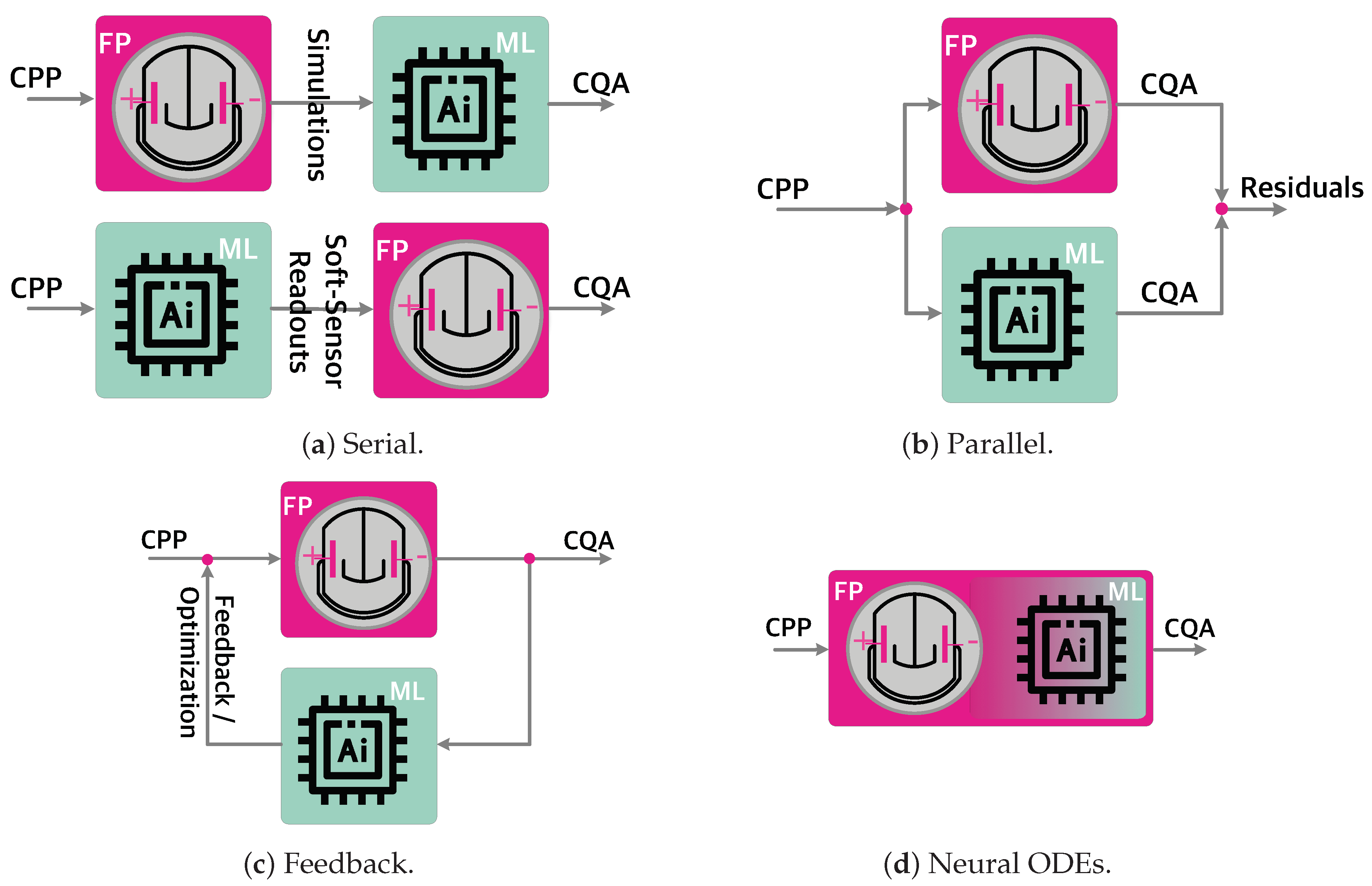
2.1. Hybrid Process Models

In the literature, the standard hybridization architecture is the combination of first-principles models and ML algorithms in serial or parallel structure and combinations thereof [28,29,30,31]; also see Figure 1. For instance, in a sequential hybrid model setting (Figure 1a), simulation results based on first-principles models are post-processed with ML algorithms for process characterization and decision making [32]. Alternatively, unknown kinetics, model parameters, system states, and process components can be reconstructed with so-called soft sensors using AI-powered, data-driven ML concepts, and sparse data might be enriched with ML-insilico data sets for process modeling [29,33,34,35,36]. These reconstructed quantities are transferred to the first-principles process model, which can only be solved or identified with the additional ML-input. In the case of a parallel setting (Figure 1b), the ML algorithm operates in parallel with the first-principles process model to quantify residuals and plant-model mismatches [30], respectively. The serial and parallel architecture primarily aim at pure forward simulations, i.e., for given CPPs (Critical Process Parameters), the CQAs (Critical Quality Attributes) are predicted, ML algorithms are also used for process optimization and control, see Figure 1c. Note that ML can either be directly utilized to solve the underlying optimization problem [34,37,38] or as part of a model-order reduction framework to reduce computational costs, i.e., the ML algorithm is part of the optimization problem itself [2,39].
Alternatively, differential equations reflecting the mathematical process model and process knowledge can be directly fused with ML algorithms (Figure 1d). When using so-called universal neural (ordinary) differential equations or physics-informed neural networks (PINNs), the neural network/ML-part completes regular ordinary differential systems (ODEs) and solves partial differential equation systems, respectively [27,40,41,42,43]. This novel hybridization strategy (i.e., ODEs where a neural network determines the vector field/derivative function), seems especially useful to efficiently replace incomplete process knowledge with learning-based methods; i.e., preserving the given model structure but improving unknown system states interactions and enabling their identification, respectively [41,44,45].
In the field of ML, neural networks play an essential role and range from the simple feed-forward neural networks, multilayer perceptron, recurrent neural networks to deep neural networks. Generally, the ith neural network layer, NNL i ( x ) : R d i 1 R d i , has N i neurons in the ith layer. Moreover, NNL i ( x ) is specified with the weight matrix, W i R d i × d i 1 , and the bias vector, b i R d i . For instance, a feed-forward neural network reads as:
input layer : NNL 0 ( x ) = x R d 0 ,
hidden layer : NNL i ( x ) = σ ( W i NNL i 1 ( x ) + b i ) R d i , 1 i I 1 ,
output layer : NNL I ( x ) = W I NNL I 1 ( x ) + b I R d I ,
where for activation functions, σ ( · ) , sigmoid or tangent functions are commonly used [46]. In hybrid modeling, the first-principles model and the used ANN affects the uncertainty propagation and sensitivity analysis problem, including deep uncertainty effects.
In what follows, all implementations were coded in Julia [47]. For the studied ANN (Section 3.1) and the neural ODEs (Section 3.2), the Flux.jl [48,49] and the DiffEqFlux.jl [50] Julia library were utilized, respectively. The Adam [51] first-order gradient-based optimization algorithm was used with the L2-norm (sum of squared errors) to train the ANN and the neural ODEs. All simulations were run on a standard desktop machine.

2.2. Global Sensitivity Analysis

Basically, in GSA the model parameters, p , and the model outcomes, y , are considered as random variables, and GSA intends to measure the amount of variance that each parameter, p [ i ] , adds to the total variance of the jth model output, σ 2 ( y [ j ] ( t ) ) [52]. The conditional variance reads as σ i 2 ( y [ j ] ( t ) | p [ i ] ) . Note that the subscript i implies that the variance is taken over all parameters with the exception of p [ i ] . The expected value of the resulting conditional variance is E i σ i 2 ( y [ j ] ( t ) | p [ i ] ) , and the subscript notation of E i indicates that the expected value is only for the parameter p [ i ] . The total output variance, σ 2 ( y [ j ] ( t ) ) , can be partitioned in two additive terms [52]. With:
σ 2 ( y [ j ] ( t ) ) = σ i 2 ( E i [ y [ j ] ( t ) | p [ i ] ] ) + E i [ σ i 2 ( y [ j ] ( t ) | p [ i ] ) ] ,
the GSA (i.e., first-order Sobol’ indices [52]) is defined as:
S [ j , i ] ( t ) = σ i 2 ( E i [ y [ j ] ( t ) | p [ i ] ] ) σ 2 ( y [ j ] ( t ) ) ,
with S ( p ) R n y × n p , and i = 1 n p S [ j , i ] ( t ) 1 , j { 1 , , n y } . For more details regarding the basic concepts of variance-based sensitivity measures and notation used, the reader is referred to [52] and references therein. Please note that in what follows, parameter uncertainties were predefined and, in the presented simulation study, are not directly based on experimental data and particular parameter identification methods, respectively. However, the proposed concept can be readily applied to experimental data. The resulting parameter uncertainties in the context of DoE using the inverse of the Fisher information matrix or sample-based (Monte-Carlo) methods [53,54]. Alternatively, parameter uncertainties could be directly quantified by implementing Bayesian parameter estimation techniques [55].

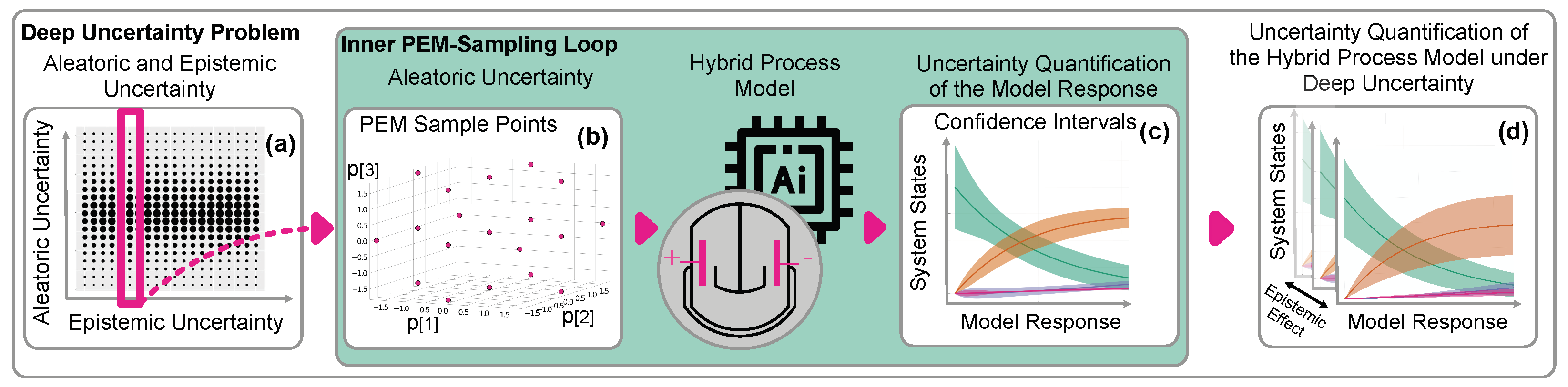
2.3. Deep Uncertainty

In the case of deep uncertainty, which besides aleatoric uncertainty, includes epistemic uncertainty, the standard UQ and GSA concepts can be extended with the parametric p-box approach [18,20,56]. Here, aleatoric uncertainties ξ depend on epistemic uncertainties θ according to:
F Ξ ( ξ ) = F Ξ ( ξ | θ ) , θ D Θ R n θ ,
where F Ξ is the cumulative distribution function (CDF) of the random vector ξ , the random vector θ with independent uniform distribution densities is specified by upper and lower bounds, and D Θ = [ θ 1 l , θ 1 u ] × [ θ n θ l , θ n θ u ] denotes the feasible domain of θ . Technically, confidence intervals might be also approximated with statistical moments [22] according to:
E θ [ E ξ [ y [ j ] ] ± β ξ σ ξ 2 [ y [ j ] ] 0.5 ] ± β θ σ θ 2 [ E ξ [ y [ j ] ] ± β ξ σ ξ 2 [ y [ j ] ] 0.5 ] 0.5 ,
where β ξ and β θ determines the conservativeness from the variation of aleatoric ξ and epistemic θ uncertainty, respectively. In this context, parameter sensitivities in terms of σ ξ 2 and σ θ 2 can be quantified with Equation (3) and the PEM.

2.4. Point Estimate Method

The basic problem with the GSA calculation, especially under deep uncertainty, is the high computational cost when approximating the underlying integral terms of Equations (2) and (3) with numerical methods, e.g., Gaussian quadrature and Monte Carlo simulations. The PEM, however, has proven advantageous for different engineering applications [57], which include sophisticated process systems engineering and electrochemical processes scenarios [58,59]. Using the nominal parameter vector p 0 , artificial but deterministic rule-based model parameter vector realizations p k result in the following parameter vector sample set, p k O : = { p 0 , O 1 , O 1 , O 2 , O 2 , O 3 , O 3 } with:
O 1 : = { p 0 [ i ] + ϑ , i { 1 , , n p } } ,
O 2 : = { p 0 [ ( i , j ) ] + [ + ϑ , + ϑ ] , i , j j > i { 1 , , n p } } ,
O 3 : = { p 0 [ ( i , j ) ] + [ ϑ , + ϑ ] , i , j j > i { 1 , , n p } } .
Note that the total parameter sample number, n P E M , scales quadratically with the number of uncertain model parameters:
n P E M = 2 n p 2 + 1 ,
and the expected value, E [ · ] , of the model response is approximated with:
E [ y ( p ) ] k = 1 n P E M w k y ( p k ) .
Here, in case of a standard Gaussian distribution, the permutation parameter and weight factors are defined as ϑ = 3 , w 0 = 1 + n p 2 7 n p 18 , w 1 , , 2 n p + 1 = 4 n p 18 , w 2 n p + 2 , , n P E M = 1 36 , respectively. As demonstrated in [60], using the PEM any parametric or non-parametric probability distribution can be incorporated via a (non)linear transformation step.
The variance, σ 2 [ · ] , can be approximated in the same way:
σ 2 [ y ( p ) ] k = 1 n P E M w k ( y ( p k ) E [ y ( p ) ] ) 2 .
Note that to consider epistemic uncertainty, an outer loop of uncertainty propagation must be implemented, e.g., the scaling factor ϑ and weights w i of the PEM are adapted to uniform probability distributions [57]. Thus, there are n P E M = 4 n θ 2 n ξ 2 + 2 ( n θ 2 + n ξ 2 ) + 1 total PEM sample points, including aleatoric and epistemic uncertainty. Moreover, due to a nested re-sampling strategy, the global sensitivity matrix (Equation (3)) can be determined highly efficiently with n P E M model simulations, where appropriate subsets, P i O , are evaluated to calculate S ( p [ i ] ) , i { 1 , , n p } . For more details regarding the general PEM in UQ and GSA, please refer to [58].
The general structure of the PEM-based approach for UQ and GSA in hybrid modeling under deep uncertainty is visualized in Figure 2.

3. Results and Discussion

Two electrochemical synthesis processes, the synthesis of furfuryl alcohol from furfural and the electrochemical reduction of nitrobenzene to 4-aminophenol, are considered in this work. The electrochemical synthesis has advantage of mild operating conditions such as temperature and pressure in comparison to the conventional chemical synthesis processes. Moreover, the reaction rate of electrochemical synthesis processes can be controlled by changing the potential/current applied during the process [61]. The modeling of electrochemical synthesis of furfuryl alcohol and 4-aminophenol are explained in Section 3.1 and Section 3.2, respectively.

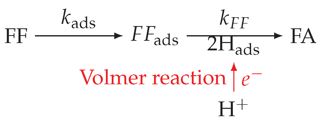
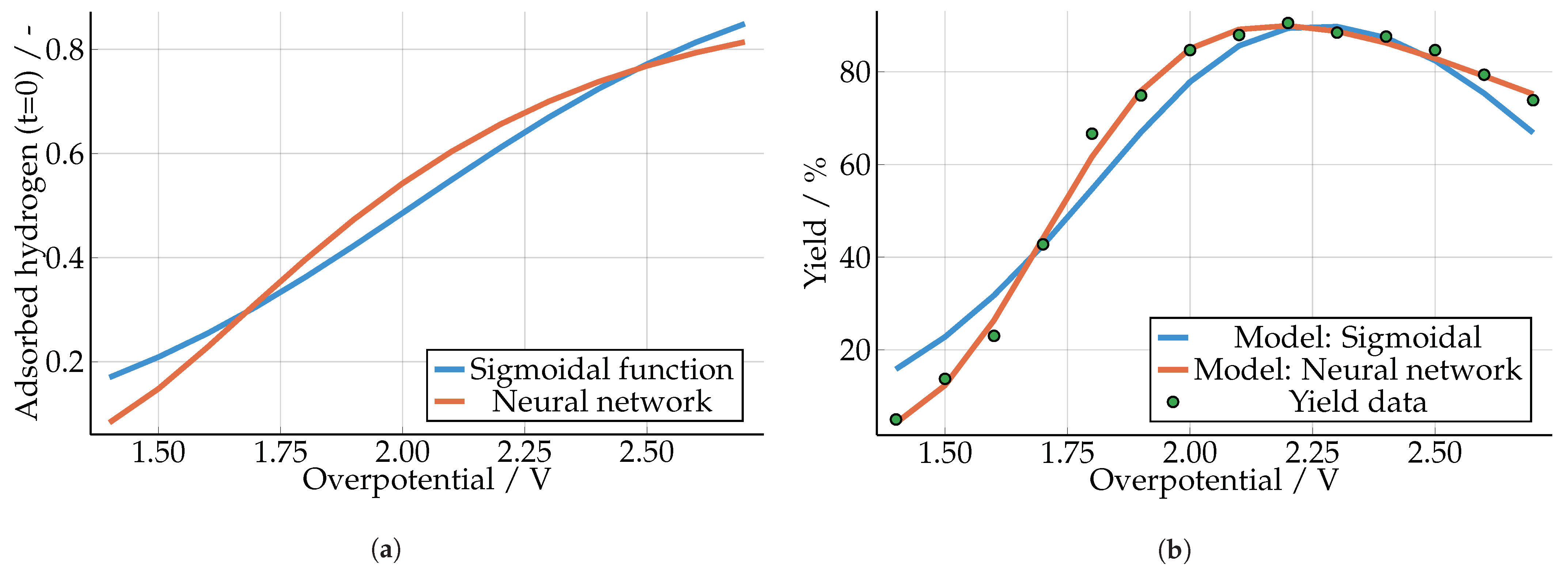
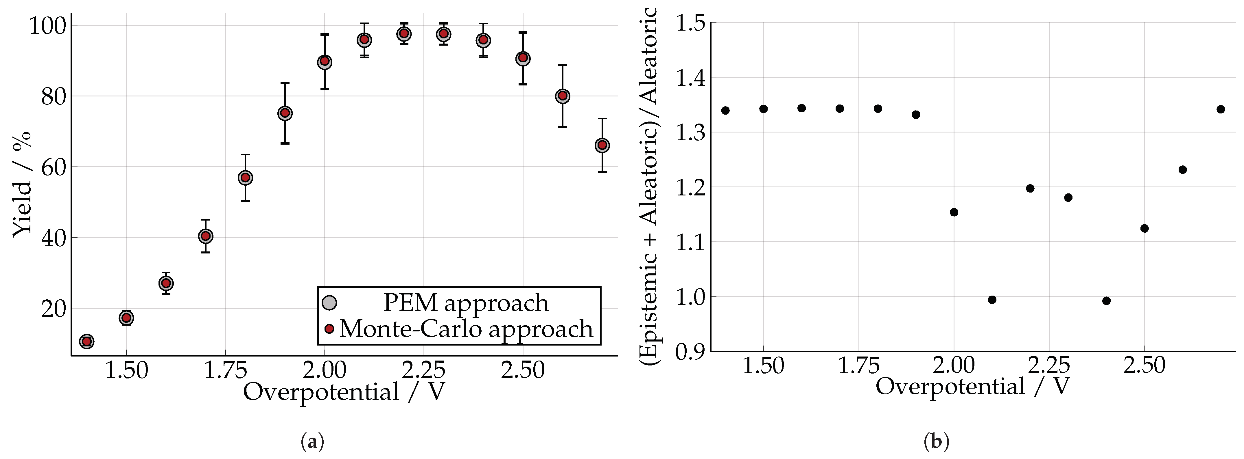
3.1. Furfuryl Alcohol with a Serial Hybrid Model

According to Figure 3, the electrochemical synthesis of furfuryl alcohol (FA) from furfural (FF) involves the formation of adsorbed hydrogen (H ads ) from a Volmer reaction, adsorption of furfural (FF ads ) on the electrode surface, and the reaction of H ads and FF ads . In what follows, the bulk concentration of all species are given in mol cm−3. To derive a simplistic first-principles process model, the following assumptions are made:
  • The hydrogen fraction of adsorbed hydrogen remains the same during the reaction (continuous reaction and negligible hydrogen evolution).
  • There is no formation of additional byproducts such as methyl furan, methyltetrahydrofuran, and tetrahydrofurfuryl alcohol.
  • The fraction of the surface area available for the reactions does not change over process time.
The governing ordinary differential equation system based on material balances for a continuous operation reads as:
d F F ads d t = C ( r ads r F F ) ,
d F F d t = Q in V F F in r ads · a Q out V F F ,
d F A d t = Q in V F A in + r F F · a Q out V F A .
In Equations (13) and (14), Q in and Q out refer to the flow rate of input and output, V refers to reactor volume and a refers to effective surface area. The rate of adsorption of FF on the electrode surface is expressed as:
r ads = k ads · F F · θ v ,
In Equation (15), k ads and θ v refer to rate constant for adsorption of FF and vacant sites available for adsorption of FF, respectively. and the rate of conversion of FF to FA is defined as:
r F F = k F F · θ H 2 · F F ads .
In Equation (16), k F F refers to rate constant for conversion of furfural to furfuryl alcohol.
The adsorption of hydrogen by the Volmer reaction, θ H , is typically represented by adsorption isotherms such as the Langmuir adsorption isotherm [62]. In this case, adsorption of hydrogen and FF are necessary for the conversion of FF to FA. As the overpotential-dependent data for θ H is not available in the literature for the system under study, a sigmoid function relating the initial adsorbed hydrogen, θ H 0 , and the overpotential, E, could be used as an empirical model in the simplest case:
θ H 0 = 1 1 + e x p ( ( s 1 + s 2 · E ) ) .
By evaluating the least squares error, the sigmoid function was parameterized; i.e., s 1 = 5.15 and s 2 = 2.55 . For a more precise calculation, the sigmoid function can be replaced with an ANN resulting in a hybrid process model framework. The overpotential-dependent formation of H ads is expressed by a two-layer ANN with six and two nodes (Equation (1)), respectively, with tangent functions as activation function, overpotential as the ANN input, and H ads as the ANN output.
The hybrid model was trained with values of yield of furfuryl alcohol for overpotentials between 1.4 to 2.7 V from literature [63]. The ANN outcome of the overpotential vs. the fraction of surface covered by H ads is shown in Figure 4a, and the process model parameters are given in Table 1. The fraction of adsorbed hydrogen increased with as the overpotential changed from 1.4 to 2.7 V since there are no other potential dependent reactions in the reaction scheme of furfuryl alcohol synthesis (Figure 4b). The concentration of furfuryl alcohol predicted by the model with the sigmoid function for hydrogen adsorption and the hybrid model were in reasonable agreement with the data from literature for the overpotential between 1.4 to 2.7 V (Figure 4b).
The impact of parameter uncertainties on the yield of furfuryl alcohol was studied using the conventional Monte-Carlo approach and the proposed PEM approach. Please note that these model parameters refer to the parameter vector p in Equations (2), (3) and (6)–(11). The range of uncertain parameters considered are given in Table 2 for epistemic uncertainty, and for aleatoric uncertainty a standard deviation of 10% of the nominal model parameters (Table 1) are assumed. The PEM approach was able to predict the impact of uncertain parameters on yield of furfuryl alcohol with less number of samples in comparison to the Monte-Carlo approach. For example, the 95%-confidence intervals (CIs) for yield of furfuryl alcohol in presence of deep uncertainty in model parameters is demonstrated in Figure 5a. The impact of uncertainties is less in the range 2.1 to 2.4 V since the process reaches almost complete conversion of furfural to furfuryl alcohol. Moreover, the impact of uncertainties were also negligible for low values of overpotential (<1.7 V ). However, operating in this range is not desirable since the yield of furfuryl alcohol is also less (<40%).
As shown in Figure 5b, the sensitivity ratio for aleatoric and epistemic uncertainty with respect to the yield of furfuryl alcohol was calculated using the PEM approach. For the range of overpotential studied (1.4 to 2.7 V ) and given statistics in Table 2, the added epistemic uncertainty increased the overall uncertainty in the predicted yield coefficients. Please note that the epistemic contribution is minor at 2.1 and 2.4 V as the process reaches complete conversion of furfural to furfuryl alcohol, and the dynamic of conversion and the increased model parameter uncertainties, respectively, have a negligible effect in consequence (Figure 5b).

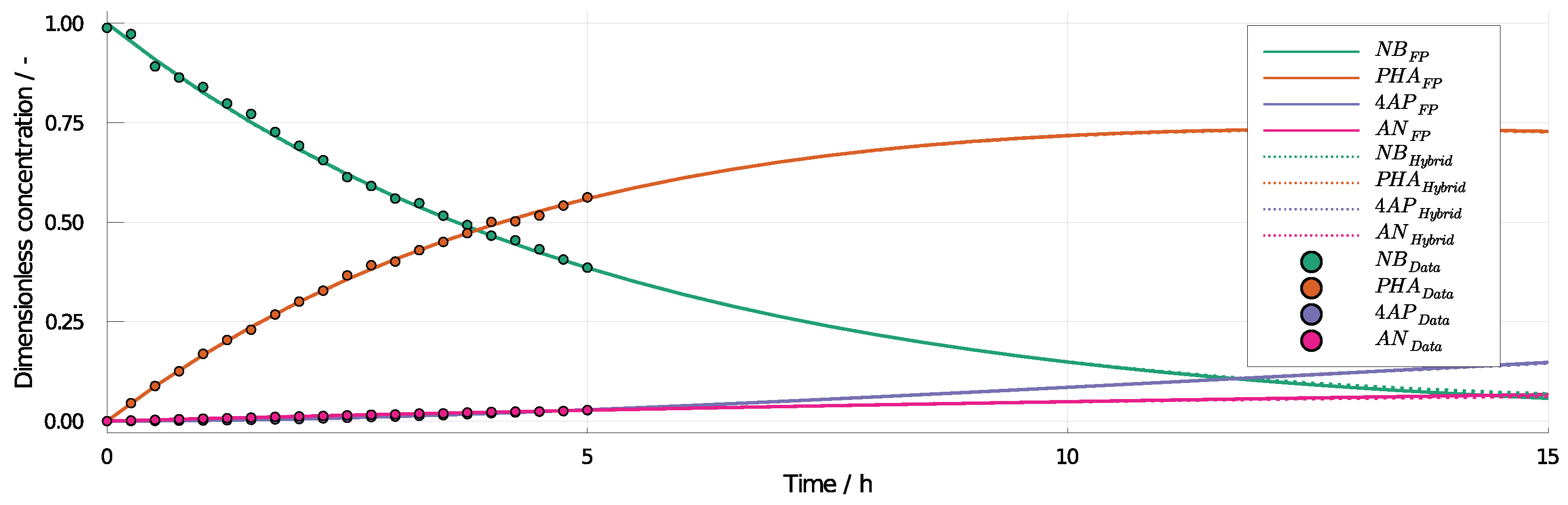
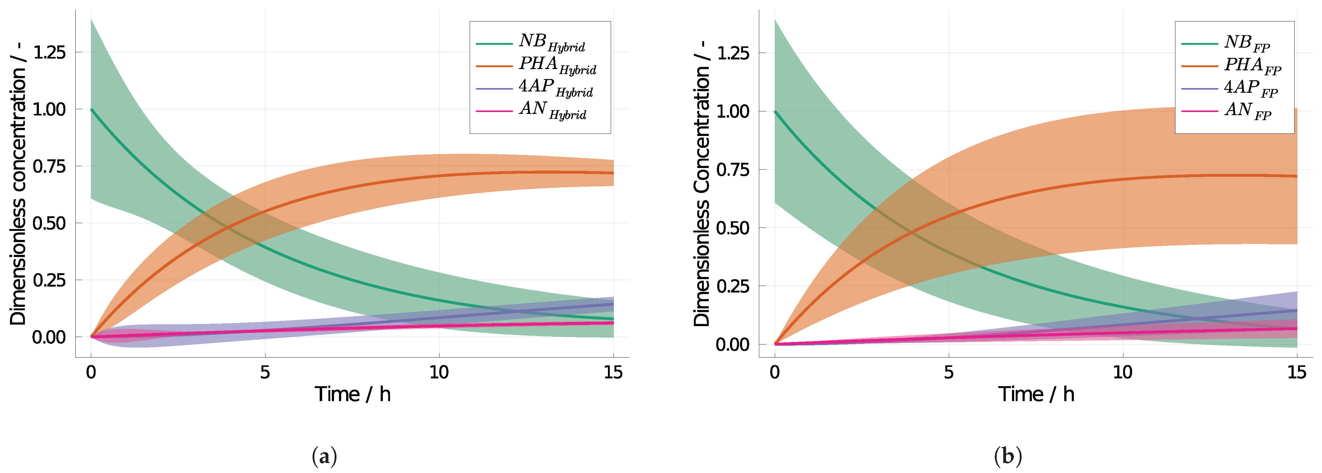
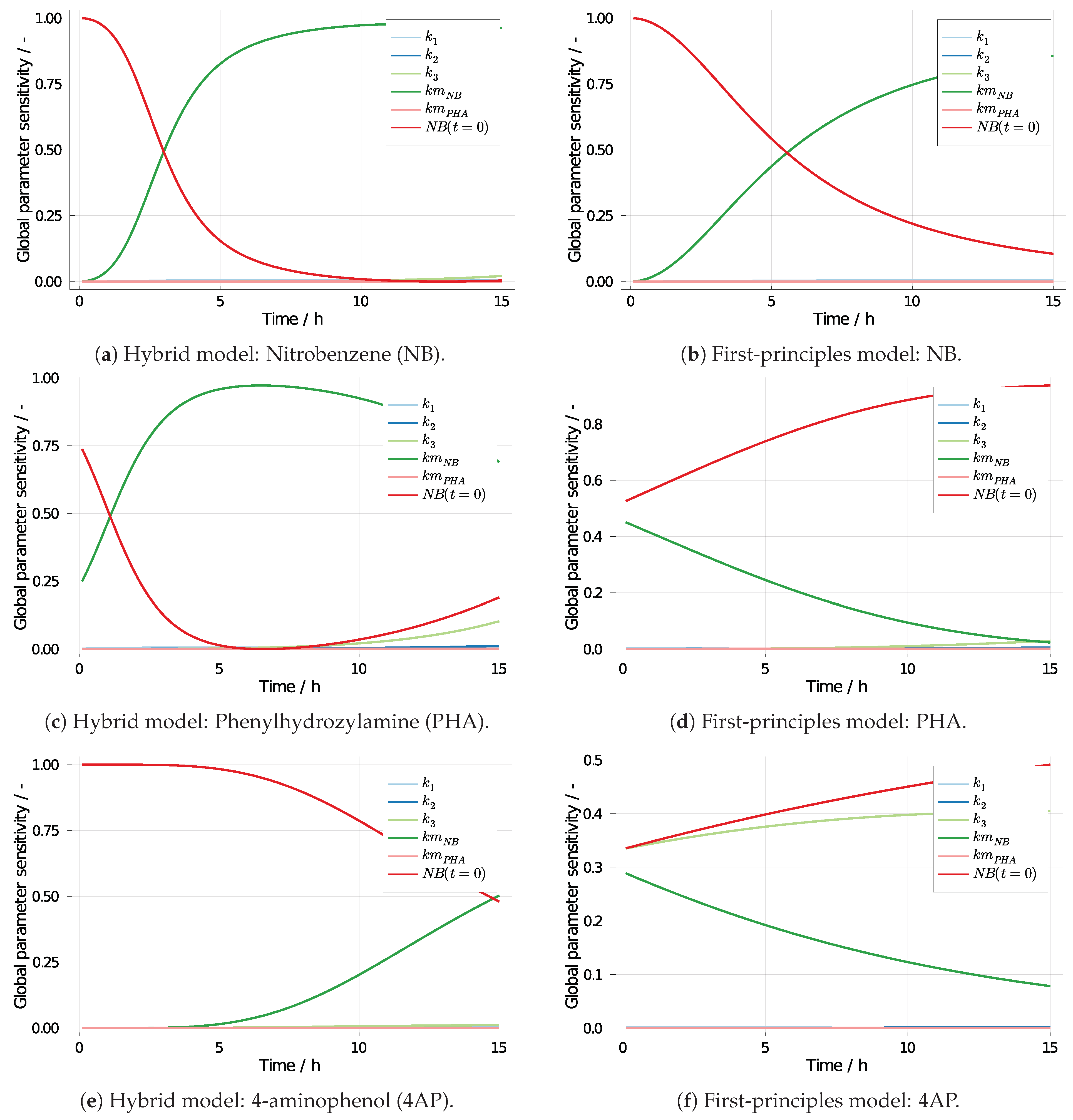
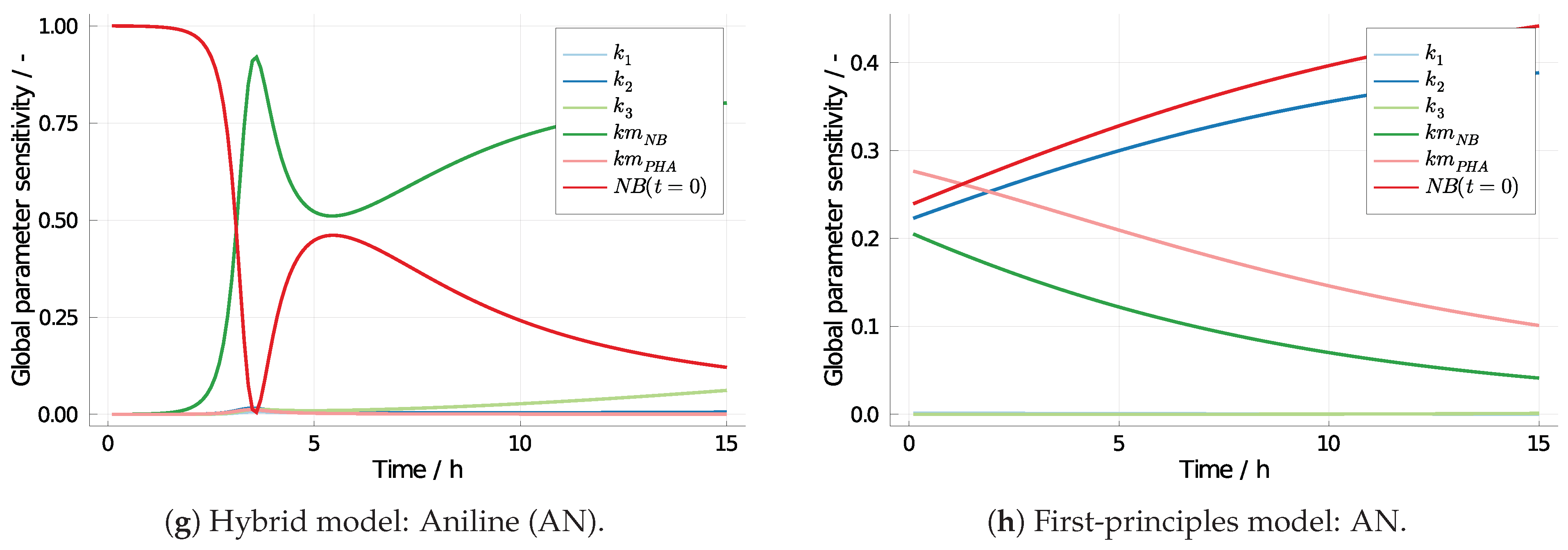
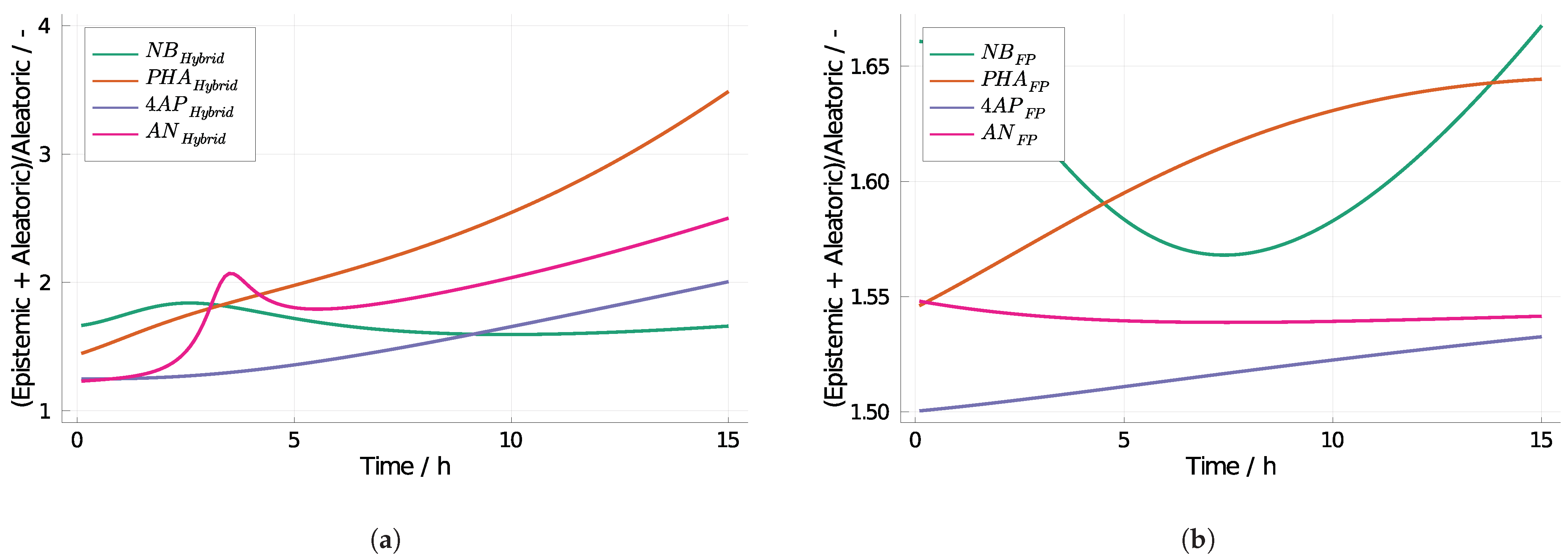
3.2. 4-Aminophenol with Neural Differential Equations

4-Aminophenol is an intermediate for the synthesis of pharmaceutical products such as paracetamol and phenacetin [64]. Typically, 4-aminophenol is synthesized through a chemical route by hydrogenation of nitrobenzene or nitration of phenol. On the other hand, 4-aminophenol can be synthesized through an electrochemical route from nitrobenzene (NB) with phenylhydroxylamine (PHA) as an intermediate [65]. The intermediate (PHA) further undergoes chemical conversion to produce 4-aminophenol (4AP) or electrochemical conversion to produce aniline (AN). In contrast to the chemical route, the electrochemical route does not use any additional toxic agents. In this work, 4-aminophenol (4AP) is considered as desired product, and AN is considered as an undesired product [66,67]. The reaction scheme for electrochemical synthesis of 4-aminophenol is given in Figure 6.
Based on Bakshi and Fedkiw [67], the material balance equations for concentration of NB, PHA, 4AP, and AN read as:
d N B d t = a · r N B ,
d P H A d t = a ( r N B r A N ) r 4 A P ,
d 4 A P d t = r 4 A P ,
d A N d t = a · r A N ,
where the rate of conversion of NB to PHA is given as:
r N B = k 1 · N B s · u c 1 ,
u c 1 = e x p ( α 1 · f · E c ) ,
f = F R T .
In Equation (23), α 1 and E c refer to the charge transfer coefficient for the desired cathodic reaction, and cathode potential, respectively. In Equation (24), R refers to gas constant and T refers to temperature. Similarly, the electrochemical synthesis of AN from PHA is expressed as:
r A N = k 2 · P H A s · u c 2 ,
u c 2 = e x p ( α 2 · f · E c ) .
In Equation (26), α 2 refers to the charge transfer coefficient for the undesired cathodic reaction. The chemical synthesis of 4AP from PHA is defined as:
r 4 A P = k 3 · P H A .
In Equations (22) and (25), N B s and P H A s refers to surface concentration of NB and PHA, respectively. The surface concentration of NB and PHA are calculated from the bulk concentration based on Equations (28) and (29), respectively.
N B s = k m N B · N B k m P H A + k 2 · u c 1 ,
P H A s = 1 k m P H A + k 2 · u c 2 × k m P H A · P H A + k 1 · u c 1 k m N B · N B k m N B + k 1 · u c 1 .
The model parameters and initial values are summarized in Table 3. Note that these model parameters refer to the parameter vector p in Equations (2), (3), and (6)–(11). Please also note that, as in the original study [66], dimensionless concentration profiles were considered. Here, the normalization is done with the NB initial concentration, N B ( t = 0 ) = 50 × 10 6 mol cm 3 ).
In the simulation study below, the original model (Equations (18)–(21)) is used as a reference and to generate simulated measurement data. Furthermore, in the context of hybrid modeling, the following neural ODE problem is considered:
d N B d t = a · r N B + A N N ( N B , P H A , 4 A P , A N ) ,
d P H A d t = a ( r N B r A N ) r 4 A P + A N N ( N B , P H A , 4 A P , A N ) ,
d 4 A P d t = A N N ( N B , P H A , 4 A P , A N ) ,
d A N d t = A N N ( N B , P H A , 4 A P , A N ) ,
where A N N ( · ) refers to a multilayer perceptron (MLP) with two hidden layers, eight nodes per hidden layer, input and output layer with 4 nodes (Equation (1)), and tangent function as activation function. Thus, Equations (30)–(33) represent limited process knowledge, i.e., knowledge is embedded in particular in Equations (30) and (31) with the kinetic expressions for r N B , r A N , and r 4 A P . The neural ODE system, however, also embeds an ANN for learning missing functions (Equations (32) and (33)) or possibly incomplete expressions (Equations (30) and (31)). Please note that the A N N ( · ) term could be used exclusively in Equations (30) and (31), i.e., assuming no process knowledge, and, alternatively, additional first-principles dependencies could be added in Equations (32) and (33), i.e., further mechanistic relationships are known.
Figure 7 shows the reference simulations (Equations (18)–(21)), the artificial measurement data calculated from them under an additive measurement noise ( σ y = 0.1 ), and the simulations of the neural ODE system (Equations (30)–(33)). For both the training phase (≤5 h ) and the prediction phase (>5 h )), the trajectories of the neural ODE system describe the reference values without any noticeable deviations. Despite the excellent fit, it should not be ignored that the simulations of both the reference model and the determined hybrid model are subject to strong uncertainties due to uncertain model parameters, including the initial value of nitrobenzene. Note that model parameters refer to the reference model and its parameters given in Table 3 which are, however, included in the neural ODE system (Equations (30) and (31)). The aleatoric model parameter uncertainties, i.e., a standard deviation of 20% of the nominal model parameters (Table 3), affect the simulations of the reference model and the hybrid model equally.
In Figure 8, the resulting 95%-CIs are illustrated assuming a Gaussian distribution; i.e., symmetric CIs. In case of the hybrid model (Figure 8a), the uncertainties in the simulation are less amplified when compared with the reference model’s CIs (Figure 8b). These differences can be explained by the fact that the interactions and interrelationships of the system states and the model parameters are not included one-to-one in the derived neural ODE system. Accordingly, although the concentration profiles can be correctly predicted deterministically using the neuronal ODEs, a realistic prediction of the uncertainties is not possible with the hybrid model. The predictions of the hybrid model, in turn, are subject to uncertainties, which have to be taken into account in the hybrid-model-based analysis.
The different behavior in uncertainty propagation of the hybrid and first-principles model is also reflected in the parameter sensitivities. In Figure 9, GSA profiles of the hybrid and the first-principles model are summarized. Similar to the uncertainty propagation problem, the model parameters k 1 , k 2 , k 3 , k m N B , and k m P H A and the initial condition of nitrobenzene N B ( t = 0 ) are considered random variables with statistics given in Table 4. In general, it can be concluded for both modeling approaches that k m N B as well as N B ( t = 0 ) have the largest impact on the simulations, and thus, correspond well with the literature [66]. However, a closer look also reveals that the temporal profiles differ significantly. For example, in the case of the concentration curve of NB, there is a time lag in the sensitivity profiles when the hybrid model (Figure 9a) is compared with the first-principles model (Figure 9b). In Figure 9c,d, even an inversion of the sensitivity profiles can be seen for the PHA trajectory. Also, sensitivity contributions of the other parameters are not correctly reproduced when studying the hybrid model; see Figure 9e–h. Similar to the uncertainty propagation itself, the hybrid model cannot be used to predict parameter sensitivities of the first-principles model and the real process, respectively. These different effects are true not only for aleatoric uncertainty but also under deep uncertainty.
In the context of deep uncertainty, epistemic uncertainty is added to aleatoric uncertainty. As can be seen from Table 4, epistemic uncertainty refers to the model parameters but also the initial value of NB, and thus, take into account higher-level kinetics variations due to degradation effects or different literature values and fluctuations in the reactants, respectively. For simplicity, the total effect is considered in the uncertainty amplification, i.e., the ratio of deep uncertainty (epistemic plus aleatoric) vs aleatoric uncertainty in the simulation results. In Figure 10, a strong uncertainty amplification can be observed for the hybrid model. The epistemic uncertainty affects the PHA prediction most, i.e., the variance values are increased by factor three. In contrast, the first-principles model is less sensitive to deep uncertainty; see Figure 10b. Although all simulation results are again influenced by the epistemic uncertainty, i.e., the uncertainties in the simulations are increased, there is only an increase of 60–65%. Note that when using Equation (5), the individual global sensitivities of the quantities given in Table 4 could be calculated, and their uncertainty fraction caused by deep uncertainty in the simulations also quantified.

3.3. Computing Effort

As discussed in the previous two case studies, good approximation results can be obtained with the PEM in the uncertainty calculation for hybrid modeling; this includes the GSA calculation and the consideration of aleatoric and epistemic uncertainties in the context of deep uncertainty. Also shown above, the PEM is a useful tool to describe and propagate uncertainties in a CPU-friendly way. The low computational cost, of course, depends on two factors: (1) the deterministic sampling scheme (Equations (6)–(8)) and (2) the re-sampling strategy for GSA using appropriate subsets, P i O , to calculate S ( p [ i ] ) , i { 1 , , n p } (Equation (3)). Thus, in the example of FA synthesis and three uncertain parameters ( n ξ = 3 ), a total of 19 sample points are generated in the parameter space, and 19 model simulations must be performed accordingly for further calculation of confidence intervals and GSA assuming aleatoric uncertainty. If for the further deep uncertainty analysis, the epistemic part is added (i.e., six parameters ( n θ = 6 ) describing the uncertainties of the uncertainties and the variance of the three considered model parameters), the total simulation effort increases to 1387 simulation runs. Similarly, in the case of the 4AP synthesis and aleatoric uncertainty, starting with six uncertain model parameters ( n ξ = 6 ) results in 73 sample points and model simulations, respectively. When adding the epistemic part under deep uncertainty ( n θ = 12 ), the overall number of model evaluations increase to 21,097 simulations. This is nevertheless a comparatively small computational effort if one compares this with the standard Monte Carlo simulations. In the case of deep uncertainty with the standard double-loop approach for uncertainty quantification, the computational effort is 10 5 simulations-solely for the determination of the confidence intervals. In the case of PEM, however, the generated parameter samples and the model simulations already allow a comprehensive calculation of global parameter sensitivities and to distinguish between aleatoric and epistemic effects on simulation results.

4. Conclusions

In the present work, it has been successfully demonstrated that hybrid modeling approaches can be usefully employed for the mathematical description of electrochemical synthesis problems, including batch and continuous operation. In terms of hybrid modeling, a standard hybrid architecture, i.e., the serial interconnection of a ML algorithm and a first-principles process model, was applied for the synthesis of furfuryl alcohol with good agreement to measurement data. Whereas for the 4-aminophenol synthesis problem, the highly topical hybrid approach of neural ODEs was successfully implemented in a simulation study. Moreover, regardless of the synthesis problem and hybridization strategy, it became clear that uncertainty quantification and parameter sensitivities are an important tool in model-based analysis when using hybrid process models. For example, confidence intervals provide possible safety limits for further process design and parameter sensitivities provide insight for improving model quality but also possible control variables for improving electrochemical synthesis performance.
With the presented case studies, it also became clear that epistemic uncertainty has a very large impact on model reliability, and thus, the issue of deep uncertainty should play an important role for holistic uncertainty analysis. However, this can only be implemented practically provided that powerful algorithms are available for uncertainty propagation and for the quantification of global parameter uncertainties. Once again, the point estimate method has proven to be an interesting and promising approach. The computational cost does not scale exponentially with the dimension of the uncertain parameters/factors under consideration. Moreover, the deterministic sampling allows for easy parallel computation and reproducible results.
For the neural ODEs, a notable effect was observed in the uncertainty propagation and parameter sensitivities. The hybrid model cannot be used to predict parameter sensitivities of the first-principles model and the real process, respectively. Rather, the GSA values must be considered separately for the specific use case. In the context of hybrid modeling, the GSA reveals the influence of the partially known process knowledge and the associated model parameters on the simulations, and thus, represent added value in themselves when interpreting hybrid process models.
This study deliberately considered the influence of model parameters in the context of hybrid modeling. The uncertainties of the meta-parameters of the ML algorithms were neglected. Ultimately, however, both the model parameters and the meta parameters have a major impact in hybrid modeling under deep uncertainty. Systematic consideration of both classes of parameters will be the subject of future research.

Author Contributions

The individual author contributions read as follows: conceptualization, R.S.; methodology, R.S.; validation, F.F.-X., F.K. and R.S.; coding, F.F.-X. and R.S.; writing—original draft preparation, F.F.-X. and R.S.; writing—review and editing, F.K. and R.S.; visualization, F.F.-X. and R.S.; supervision, R.S.; funding acquisition, R.S. All authors have read and agreed to the published version of the manuscript.

Funding

The authors would like to acknowledge the funding by the Deutsche Forschungsgemeinschaft (DFG, German Research Foundation) under Germany’s Excellence Strategy–EXC 2163/1- Sustainable and Energy Efficient Aviation–Project-ID 390881007. Furthermore, the authors acknowledge support by the German Research Foundation and the Open Access Publication Funds of Technische Universität Braunschweig.

Conflicts of Interest

The authors declare no conflict of interest. The funders had no role in the design of the study; in the collection, analyses, or interpretation of data; in the writing of the manuscript, or in the decision to publish the results.

References

  1. Nielsen, R.F.; Nazemzadeh, N.; Sillesen, L.W.; Andersson, M.P.; Gernaey, K.V.; Mansouri, S.S. Hybrid machine learning assisted modelling framework for particle processes. Comput. Chem. Eng. 2020, 140, 106916. [Google Scholar] [CrossRef]
  2. Schäfer, P.; Caspari, A.; Schweidtmann, A.M.; Vaupel, Y.; Mhamdi, A.; Mitsos, A. The Potential of Hybrid Mechanistic/Data-Driven Approaches for Reduced Dynamic Modeling: Application to Distillation Columns. Chem. Ing. Tech. 2020, 92, 1910–1920. [Google Scholar] [CrossRef]
  3. Asprion, N.; Böttcher, R.; Pack, R.; Stavrou, M.E.; Höller, J.; Schwientek, J.; Bortz, M. Gray-Box Modeling for the Optimization of Chemical Processes. Chem. Ing. Tech. 2019, 91, 305–313. [Google Scholar] [CrossRef]
  4. Chen, Y.; Yang, O.; Sampat, C.; Bhalode, P.; Ramachandran, R.; Ierapetritou, M. Digital Twins in Pharmaceutical and Biopharmaceutical Manufacturing: A Literature Review. Processes 2020, 8, 1088. [Google Scholar] [CrossRef]
  5. Noll, P.; Henkel, M. History and Evolution of Modeling in Biotechnology: Modeling & Simulation, Application and Hardware Performance. Comput. Struct. Biotechnol. J. 2020, 18, 3309–3323. [Google Scholar] [CrossRef]
  6. Krippl, M.; Dürauer, A.; Duerkop, M. Hybrid modeling of cross-flow filtration: Predicting the flux evolution and duration of ultrafiltration processes. Sep. Purif. Technol. 2020, 248, 117064. [Google Scholar] [CrossRef]
  7. Cardillo, A.G.; Castellanos, M.M.; Desailly, B.; Dessoy, S.; Mariti, M.; Portela, R.M.C.; Scutella, B.; von Stosch, M.; Tomba, E.; Varsakelis, C. Towards in silico Process Modeling for Vaccines. Trends Biotechnol. 2021. [Google Scholar] [CrossRef]
  8. Hotvedt, M.; Grimstad, B.; Imsland, L. Identifiability and interpretability of hybrid, gray-box models. arXiv 2020, arXiv:2010.13416. [Google Scholar]
  9. Feng, J.; Lansford, J.L.; Katsoulakis, M.A.; Vlachos, D.G. Explainable and trustworthy artificial intelligence for correctable modeling in chemical sciences. Sci. Adv. 2020, 6, 1–11. [Google Scholar] [CrossRef]
  10. Bayer, B.; Striedner, G.; Duerkop, M. Hybrid Modeling and Intensified DoE: An Approach to Accelerate Upstream Process Characterization. Biotechnol. J. 2020, 15, 2000121. [Google Scholar] [CrossRef]
  11. Kiureghian, A.D.; Ditlevsen, O. Aleatory or epistemic? Does it matter? Struct. Saf. 2009, 31, 105–112. [Google Scholar] [CrossRef]
  12. Urbina, A.; Mahadevan, S.; Paez, T.L. Quantification of margins and uncertainties of complex systems in the presence of aleatoric and epistemic uncertainty. Reliab. Eng. Syst. Saf. 2011, 96, 1114–1125. [Google Scholar] [CrossRef]
  13. Zhang, J.; Shields, M.D. On the quantification and efficient propagation of imprecise probabilities resulting from small datasets. Mech. Syst. Signal Process. 2018, 98, 465–483. [Google Scholar] [CrossRef]
  14. Senge, R.; Bösner, S.; Dembczyński, K.; Haasenritter, J.; Hirsch, O.; Donner-Banzhoff, N.; Hüllermeier, E. Reliable classification: Learning classifiers that distinguish aleatoric and epistemic uncertainty. Inf. Sci. 2014, 255, 16–29. [Google Scholar] [CrossRef] [Green Version]
  15. Pearce, T.; Leibfried, F.; Brintrup, A.; Zaki, M.; Neely, A. Uncertainty in Neural Networks: Approximately Bayesian Ensembling. arXiv 2018, arXiv:1810.05546. [Google Scholar]
  16. Hüllermeier, E.; Waegeman, W. Aleatoric and Epistemic Uncertainty in Machine Learning: An Introduction to Concepts and Methods. Mach. Learn. 2019, 110, 1–52. [Google Scholar]
  17. Salimbeni, H.; Dutordoir, V.; Hensman, J.; Deisenroth, M.P. Deep gaussian processes with importance-weighted variational inference. In Proceedings of the 36th International Conference on Machine Learning, ICML 2019, Long Beach, CA, USA, 9–15 June 2019; pp. 9801–9810. [Google Scholar]
  18. Faes, M.; Daub, M.; Beer, M. Engineering analysis with imprecise probabilities: A state-of-the-art review on P-boxes. In Proceedings of the 7th Asian-Pacific Symposium on Structural Reliability and its Applications, University of Tokyo, Tokyo, Japan, 5–7 October 2020. [Google Scholar]
  19. Razavi, S.; Jakeman, A.; Saltelli, A.; Prieur, C.; Iooss, B.; Borgonovo, E.; Plischke, E.; Lo Piano, S.; Iwanaga, T.; Becker, W.; et al. The Future of Sensitivity Analysis: An essential discipline for systems modeling and policy support. Environ. Model. Softw. 2021, 137, 104954. [Google Scholar] [CrossRef]
  20. Beer, M.; Ferson, S.; Kreinovich, V. Imprecise probabilities in engineering analyses. Mech. Syst. Signal Process. 2013, 37, 4–29. [Google Scholar] [CrossRef] [Green Version]
  21. Schöbi, R.; Sudret, B. Structural reliability analysis for p-boxes using multi-level meta-models. Probabilistic Eng. Mech. 2017, 48, 27–38. [Google Scholar] [CrossRef] [Green Version]
  22. Xie, X.; Schenkendorf, R. Robust Process Design in Pharmaceutical Manufacturing under Batch-to-Batch Variation. Processes 2019, 7, 509. [Google Scholar] [CrossRef] [Green Version]
  23. Schöbi, R.; Sudret, B. Uncertainty propagation of p-boxes using sparse polynomial chaos expansions. J. Comput. Phys. 2017, 339, 307–327. [Google Scholar] [CrossRef] [Green Version]
  24. Bi, S.; Broggi, M.; Wei, P.; Beer, M. The Bhattacharyya distance: Enriching the P-box in stochastic sensitivity analysis. Mech. Syst. Signal Process. 2019, 129, 265–281. [Google Scholar] [CrossRef]
  25. Chen, R.T.Q.; Rubanova, Y.; Bettencourt, J.; Duvenaud, D. Neural Ordinary Differential Equations. arXiv 2018, arXiv:1806.07366. [Google Scholar]
  26. Massaroli, S.; Poli, M.; Park, J.; Yamashita, A.; Asama, H. Dissecting Neural ODEs. arXiv 2020, arXiv:2002.08071. [Google Scholar]
  27. De Jaegher, B.; Larumbe, E.; De Schepper, W.; Verliefde, A.; Nopens, I. Colloidal fouling in electrodialysis: A neural differential equations model. Sep. Purif. Technol. 2020, 249, 116939. [Google Scholar] [CrossRef]
  28. Von Stosch, M.; Oliveira, R.; Peres, J.; de Azevedo, S.F. Hybrid semi-parametric modeling in process systems engineering: Past, present and future. Comput. Chem. Eng. 2014, 60, 86–101. [Google Scholar] [CrossRef] [Green Version]
  29. Qin, S.J.; Chiang, L.H. Advances and opportunities in machine learning for process data analytics. Comput. Chem. Eng. 2019, 126, 465–473. [Google Scholar] [CrossRef]
  30. Chen, Y.; Ierapetritou, M. A framework of hybrid model development with identification of plant-model mismatch. AIChE J. 2020, 66, 1–16. [Google Scholar] [CrossRef]
  31. Aykol, M.; Balaji Gopal, C.; Anapolsky, A.; Herring, P.K.; van Vlijmen, B.; Berliner, M.D.; Bazant, M.Z.; Braatz, R.D.; Chueh, W.; Storey, B.D. Perspective—Combining Physics and Machine Learning to Predict Battery Lifetime. J. Electrochem. Soc. 2021. [Google Scholar] [CrossRef]
  32. Harting, N.; Schenkendorf, R.; Wolff, N.; Krewer, U. State-of-Health identification of Lithium-ion batteries based on Nonlinear Frequency Response Analysis: First steps with machine learning. Appl. Sci. 2018, 8, 821. [Google Scholar] [CrossRef] [Green Version]
  33. Bhutani, N.; Rangaiah, G.P.; Ray, A.K. First-Principles, Data-Based, and Hybrid Modeling and Optimization of an Industrial Hydrocracking Unit. Ind. Eng. Chem. Res. 2006, 45, 7807–7816. [Google Scholar] [CrossRef]
  34. Shang, C.; You, F. Data Analytics and Machine Learning for Smart Process Manufacturing: Recent Advances and Perspectives in the Big Data Era. Engineering 2019, 5, 1010–1016. [Google Scholar] [CrossRef]
  35. Bikmukhametov, T.; Jäschke, J. Combining machine learning and process engineering physics towards enhanced accuracy and explainability of data-driven models. Comput. Chem. Eng. 2020, 138. [Google Scholar] [CrossRef]
  36. Chen, Z.S.; Zhu, Q.X.; Xu, Y.; He, Y.L.; Su, Q.L.; Chen, Z.S. Integrating virtual sample generation with input-training neural network for solving small sample size problems: Application to purified terephthalic acid solvent system. Soft Comput. 2021, 4. [Google Scholar] [CrossRef]
  37. Lee, J.H.; Shin, J.; Realff, M.J. Machine learning: Overview of the recent progresses and implications for the process systems engineering field. Comput. Chem. Eng. 2018, 114, 111–121. [Google Scholar] [CrossRef]
  38. Petsagkourakis, P.; Sandoval, I.O.; Bradford, E.; Zhang, D.; del Rio-Chanona, E.A. Reinforcement learning for batch bioprocess optimization. Comput. Chem. Eng. 2020, 133, 106649. [Google Scholar] [CrossRef] [Green Version]
  39. Lüthje, J.T.; Schulze, J.C.; Caspari, A.; Mhamdi, A.; Mitsos, A.; Schäfer, P. Adaptive Learning of Hybrid Models for Nonlinear Model Predictive Control of Distillation Columns. arXiv 2020, arXiv:2011.12798. [Google Scholar]
  40. Chen, R.T.; Rubanova, Y.; Bettencourt, J.; Duvenaud, D.K. Neural ordinary differential equations. In Proceedings of the Advances in Neural Information Processing Systems, Montreal, QC, Canada, 3–8 December 2018; pp. 6571–6583. [Google Scholar]
  41. Rackauckas, C.; Ma, Y.; Martensen, J.; Warner, C.; Zubov, K.; Supekar, R.; Skinner, D.; Ramadhan, A. Universal differential equations for scientific machine learning. arXiv 2020, arXiv:2001.04385. [Google Scholar]
  42. Teshima, T.; Tojo, K.; Ikeda, M.; Ishikawa, I.; Oono, K. Universal Approximation Property of Neural Ordinary Differential Equations. arXiv 2020, arXiv:2012.02414. [Google Scholar]
  43. Arnold, F.; King, R. State–space modeling for control based on physics-informed neural networks. Eng. Appl. Artif. Intell. 2021, 101, 104195. [Google Scholar] [CrossRef]
  44. Champion, K.; Lusch, B.; Kutz, J.N.; Brunton, S.L. Data-driven discovery of coordinates and governing equations. Proc. Natl. Acad. Sci. USA 2019, 116, 22445–22451. [Google Scholar] [CrossRef] [Green Version]
  45. Quaghebeur, W.; Nopens, I.; De Baets, B. Incorporating Unmodeled Dynamics Into First-Principles Models Through Machine Learning. IEEE Access 2021, 9, 22014–22022. [Google Scholar] [CrossRef]
  46. Bishop, C.M. Pattern Recognition and Machine Learning; Springer: New York, NY, USA, 2006. [Google Scholar]
  47. Bezanson, J.; Edelman, A.; Karpinski, S.; Shah, V.B. Julia: A fresh approach to numerical computing. SIAM Rev. 2017, 59, 65–98. [Google Scholar] [CrossRef] [Green Version]
  48. Innes, M.; Saba, E.; Fischer, K.; Gandhi, D.; Rudilosso, M.C.; Joy, N.M.; Karmali, T.; Pal, A.; Shah, V. Fashionable Modelling with Flux. arXiv 2018, arXiv:1811.01457. [Google Scholar]
  49. Innes, M. Flux: Elegant Machine Learning with Julia. J. Open Source Softw. 2018. [Google Scholar] [CrossRef] [Green Version]
  50. Rackauckas, C.; Innes, M.; Ma, Y.; Bettencourt, J.; White, L.; Dixit, V. Diffeqflux.jl-A julia library for neural differential equations. arXiv 2019, arXiv:1902.02376. [Google Scholar]
  51. Kingma, D.P.; Ba, J. Adam: A Method for Stochastic Optimization. arXiv 2017, arXiv:1412.6980. [Google Scholar]
  52. Saltelli, A.; Ratto, M.; Tarantola, S.; Campolongo, F. Sensitivity analysis for chemical Models. Chem. Rev. 2005, 105, 2811–2828. [Google Scholar] [CrossRef]
  53. Joshi, M.; Seidel-Morgenstern, A.; Kremling, A. Exploiting the bootstrap method for quantifying parameter confidence intervals in dynamical systems. Metab. Eng. 2006, 8, 447–455. [Google Scholar] [CrossRef]
  54. Krausch, N.; Barz, T.; Sawatzki, A.; Gruber, M.; Kamel, S.; Neubauer, P.; Cruz Bournazou, M.N. Monte Carlo Simulations for the Analysis of Non-linear Parameter Confidence Intervals in Optimal Experimental Design. Front. Bioeng. Biotechnol. 2019, 7, 1–16. [Google Scholar] [CrossRef]
  55. van de Schoot, R.; Depaoli, S.; King, R.; Kramer, B.; Märtens, K.; Tadesse, M.G.; Vannucci, M.; Gelman, A.; Veen, D.; Willemsen, J.; et al. Bayesian statistics and modelling. Nat. Rev. Methods Primers 2021, 1. [Google Scholar] [CrossRef]
  56. Faes, M.; Daub, M.; Marelli, S.; Patelli, E.; Beer, M. Engineering Analysis with Probability Boxes: A Review on Computational Methods. Preprint submitted to Elsevier. 2021. [Google Scholar]
  57. Lerner, U.N. Hybrid Bayesian Networks for Reasoning about Complex Systems. Technical Report. Ph.D. Thesis, Stanford University, Stanford, CA, USA, 2002. [Google Scholar]
  58. Schenkendorf, R.; Xie, X.; Rehbein, M.; Scholl, S.; Krewer, U. The Impact of Global Sensitivities and Design Measures in Model-Based Optimal Experimental Design. Processes 2018, 6, 27. [Google Scholar] [CrossRef] [Green Version]
  59. Laue, V.; Schmidt, O.; Dreger, H.; Xie, X.; Röder, F.; Schenkendorf, R.; Kwade, A.; Krewer, U. Model-Based Uncertainty Quantification for the Product Properties of Lithium-Ion Batteries. Energy Technol. 2019, 8, 1900201. [Google Scholar] [CrossRef]
  60. Xie, X.; Krewer, U.; Schenkendorf, R. Robust optimization of dynamical systems with correlated random variables using the point estimate method. IFAC-PapersOnLine 2018, 51, 427–432. [Google Scholar] [CrossRef]
  61. Kwon, Y.; Schouten, K.J.P.; van der Waal, J.C.; de Jong, E.; Koper, M.T.M. Electrocatalytic Conversion of Furanic Compounds. ACS Catal. 2016, 6, 6704–6717. [Google Scholar] [CrossRef]
  62. Lasia, A. Influence of adsorption of organic compounds and surface heterogeneity on the hydrogen evolution reaction. Can. J. Chem. 1997, 75, 1615–1623. [Google Scholar] [CrossRef]
  63. Cao, Y.; Noël, T. Efficient Electrocatalytic Reduction of Furfural to Furfuryl Alcohol in a Microchannel Flow Reactor. Org. Process Res. Dev. 2019, 23, 403–408. [Google Scholar] [CrossRef] [PubMed] [Green Version]
  64. Vaidya, M.J.; Kulkarni, S.M.; Chaudhari, R.V. Synthesis of p-Aminophenol by Catalytic Hydrogenation of p-Nitrophenol. Org. Process Res. Dev. 2003, 7, 1083–6160. [Google Scholar] [CrossRef]
  65. Tranchant, M.; Serrà, A.; Gunderson, C.; Bertero, E.; García-Amorós, J.; Gómez, E.; Michler, J.; Philippe, L. Efficient and green electrochemical synthesis of 4-aminophenol using porous Au micropillars. Appl. Catal. A Gen. 2020, 602, 117698. [Google Scholar] [CrossRef]
  66. Bakshi, R.; Fedkiw, P. Optimal time-varying potential control. J. Appl. Electrochem. 1993, 23, 715–727. [Google Scholar] [CrossRef]
  67. Bakshi, R.; Fedkiw, P. Optimal time-varying cell-voltage control of a parallel-plate reactor. J. Appl. Electrochem. 1994, 24, 1116–1123. [Google Scholar] [CrossRef]
Figure 1. Hybrid model architectures with first-principles (FP) process model and machine learning (ML) algorithm.
Processes 09 00704 g001
Figure 2. Deep uncertainty effect in hybrid modeling. For a specific epistemic uncertainty realization (a), an aleatoric uncertainty is defined and sample points selected (b). An uncertain hybrid model response is recorded (c). Due to epistemic uncertainty various realizations are derived (d) and used for UQ and GSA.
Processes 09 00704 g002
Figure 3. Reaction scheme for electrochemical synthesis of furfuryl alcohol (FA) (red arrows represent electrochemical reactions and black arrow represent chemical reaction).
Processes 09 00704 g003
Figure 4. Comparison of sigmoidal function and neural network. (a) Fraction of adsorbed hydrogen predicted. (b) Yield of furfuryl alcohol.
Processes 09 00704 g004
Figure 5. Uncertainty propagation and sensitivity analysis for electrochemical synthesis of furfuryl alcohol. (a) CIs based on deep uncertainty. (b) Sensitivity ratio under deep uncertainty.
Processes 09 00704 g005
Figure 6. Reaction scheme for electrochemical synthesis of 4-aminophenol (4AP) (red arrows represent electrochemical reactions and black arrow represent chemical reaction).
Processes 09 00704 g006
Figure 7. Trained universal neural differential equations of the 4-aminophenol synthesis model, including the first-principles model as reference and simulated training data (training ≤ 5 h, prediction > 5 h).
Processes 09 00704 g007
Figure 8. Mean values and 95%-confidence intervals of the system states of the 4-aminophenol synthesis model under aleatoric uncertainty. (a) Hybrid model. (b) First-principles model.
Processes 09 00704 g008
Figure 9. Global parameter sensitivities of the 4-aminophenol synthesis model under aleatoric uncertainty.
Processes 09 00704 g009aProcesses 09 00704 g009b
Figure 10. Epistemic uncertainty effect in deep uncertainty of the of the 4-aminophenol synthesis model. (a) System states of the hybrid model. (b) System states of the first-principles model.
Processes 09 00704 g010
Table 1. Model parameters and initial value for electrochemical synthesis of furfuryl alcohol.
Parameter k ads k FF C FF ( t = 0 ) FA ( t = 0 ) θ H 0
Value0.5969 5.6437 × 10 8 1.6081 × 10 9 0.1 × 10 3 0Equation (17)
Unitcm s−1s−1-mol cm−3mol cm−3-
Table 2. Epistemic uncertainties of the furfuryl alcohol synthesis model assuming uniform random variables.
ParameterMeanStandard Deviation
k ads [0.5372, 0.6566][0.0537, 0.0656]
k F F [5.07  × 10 8 , 6.20  × 10 8 ][0.50  × 10 8 , 0.62  × 10 8 ]
C[1.4  × 10 9 , 1.7  × 10 9 ][1.4 × 10 8 , 1.7  × 10 8 ]
Table 3. Model parameters and dimensionless initial values for electrochemical synthesis of 4-aminophenol.
Parameter k 1 k 2 k 3 α 1 α 2 a E c
Value 6.03 × 10 8 2.71 × 10 8 4.77 × 10 6 0.6930.3980.020.5
Unitcm s−1cm s−1s−1--/ V
Parameter k mNB k mPHA fNB (t = 0)PHA (t = 0)4AP (t = 0)AN (t = 0)
Value 2.84 × 10 3 1.73 × 10 3 38.661000
Unitcm s−1cm s−1V−1----
Table 4. Epistemic uncertainties of the 4-aminophenol synthesis model assuming uniform random variables.
ParameterMeanStandard Deviation
k 1 [ 4.82 × 10 8 , 7.23 × 10 8 ][ 0.482 × 10 8 , 0.723 × 10 8 ]
k 2 [ 2.16 × 10 8 , 3.25 × 10 8 ][ 0.216 × 10 8 , 0.325 × 10 8 ]
k 3 [ 3.81 × 10 6 , 5.72 × 10 6 ][ 0.381 × 10 6 , 0.572 × 10 6 ]
k m N B [ 2.27 × 10 3 , 3.40 × 10 3 ][ 0.227 × 10 3 , 0.340 × 10 3 ]
k m P H A [ 1.38 × 10 3 , 2.07 × 10 3 ][ 0.138 × 10 3 , 0.207 × 10 3 ]
N B ( t = 0 ) [0.8, 1.2][0.08, 0.12]
Publisher’s Note: MDPI stays neutral with regard to jurisdictional claims in published maps and institutional affiliations.

