
Numerical Analysis of Hydrodynamic Loads on Passing and Moored Ships in Shallow Water

Abstract
:1. Introduction
2. Numerical Method
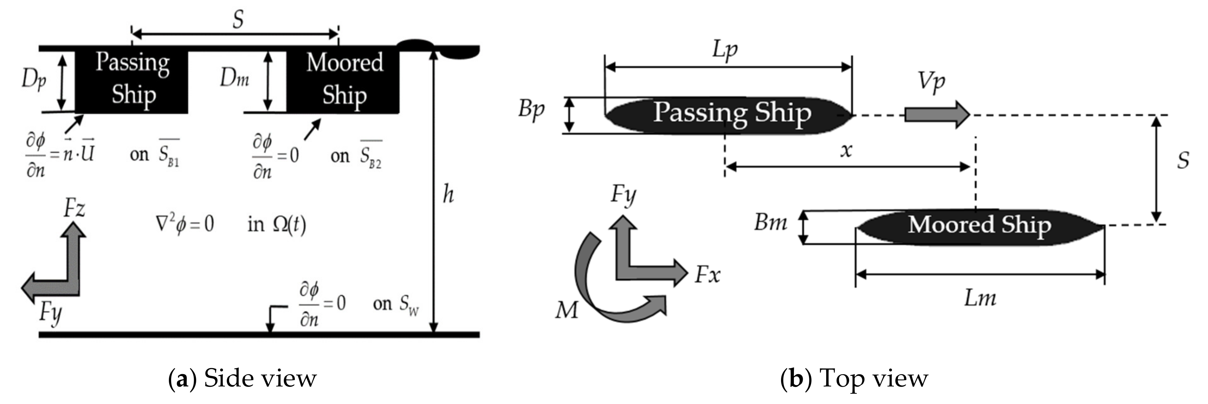
2.1. Boundary Value Problem
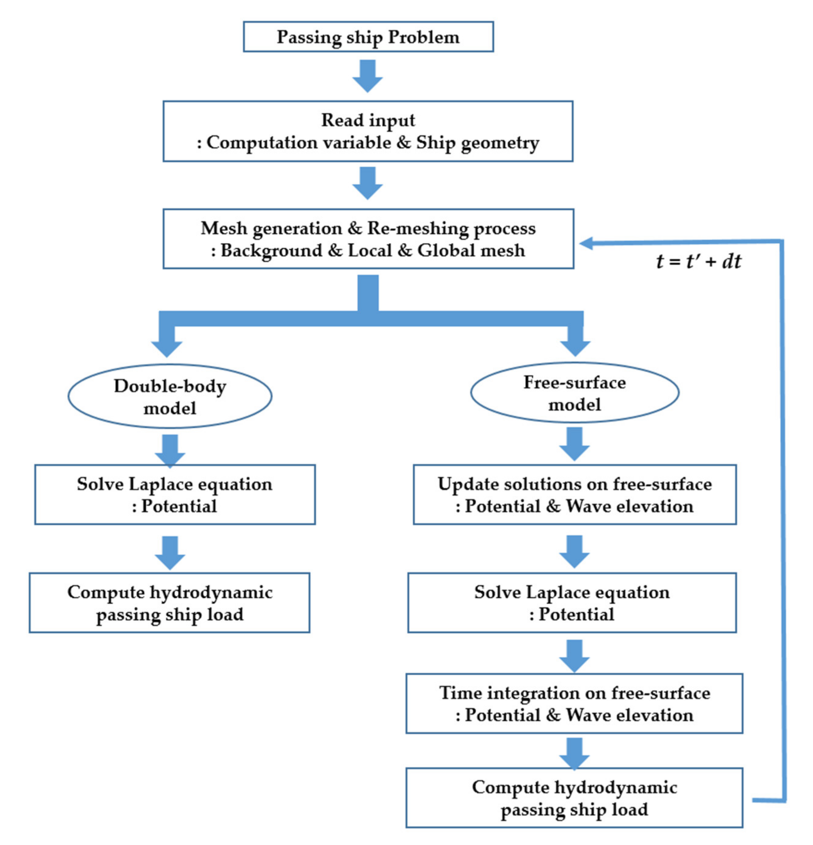
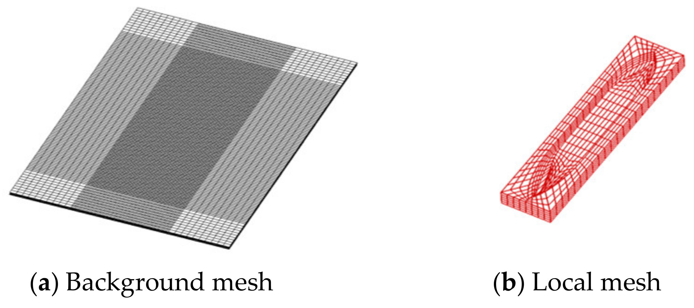
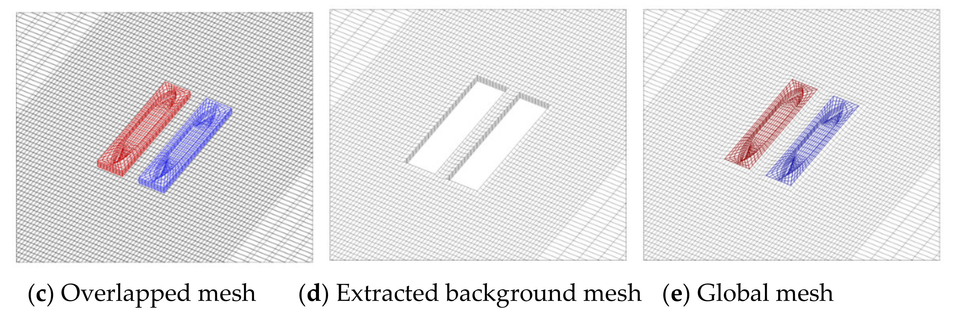
2.2. Numerical Method: Finite Element Method
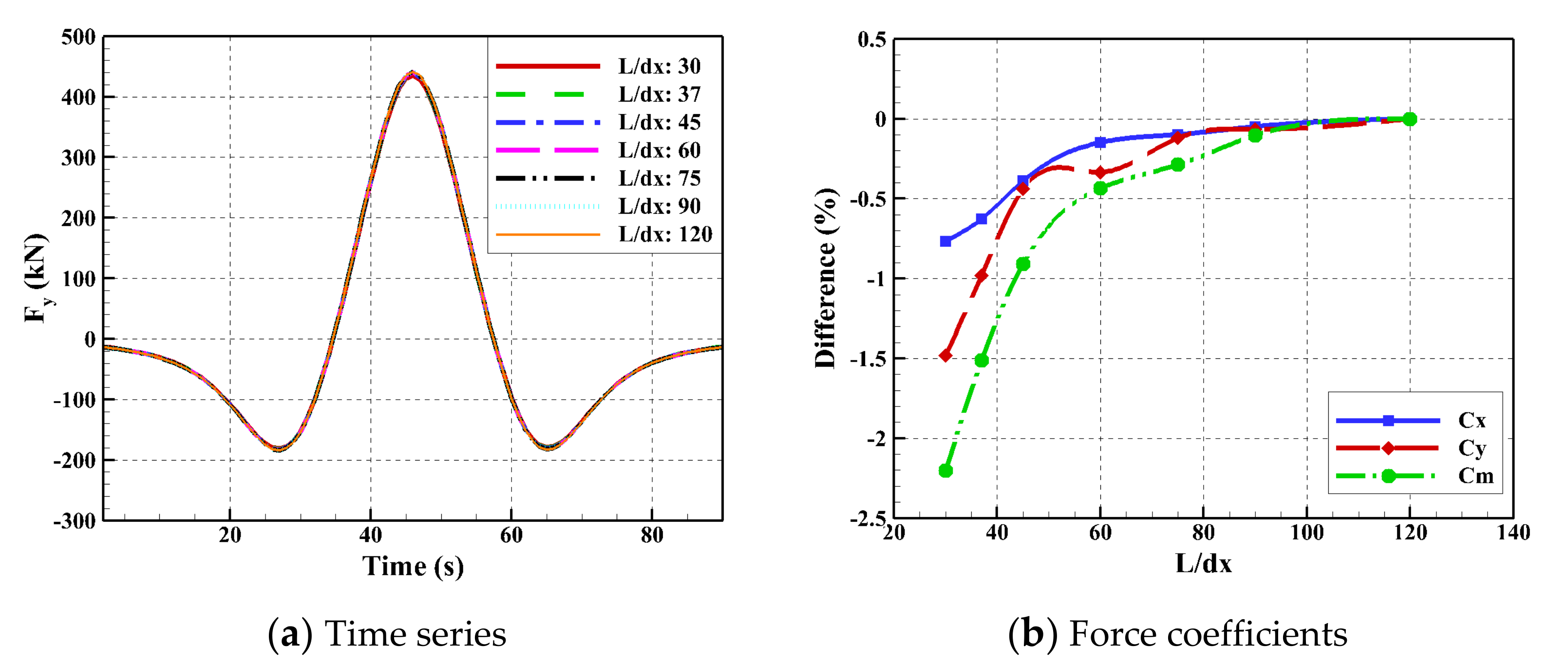
2.3. Convergence Study
2.4. Simulation Description
3. Simulation Results and Discussions
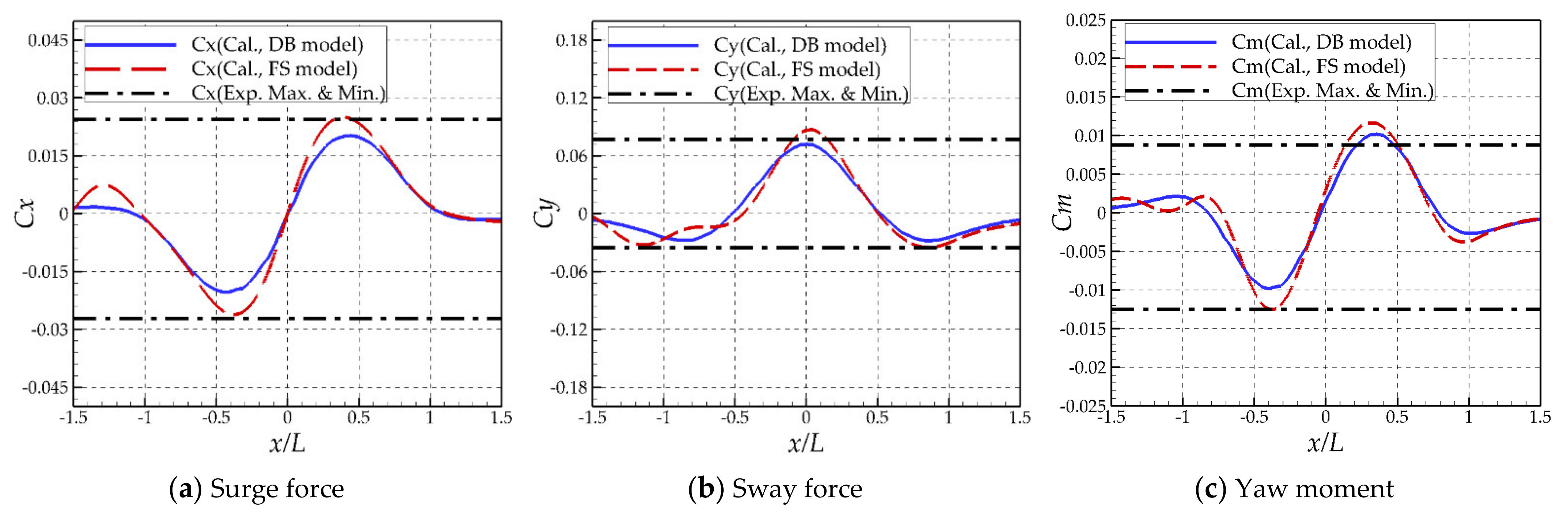
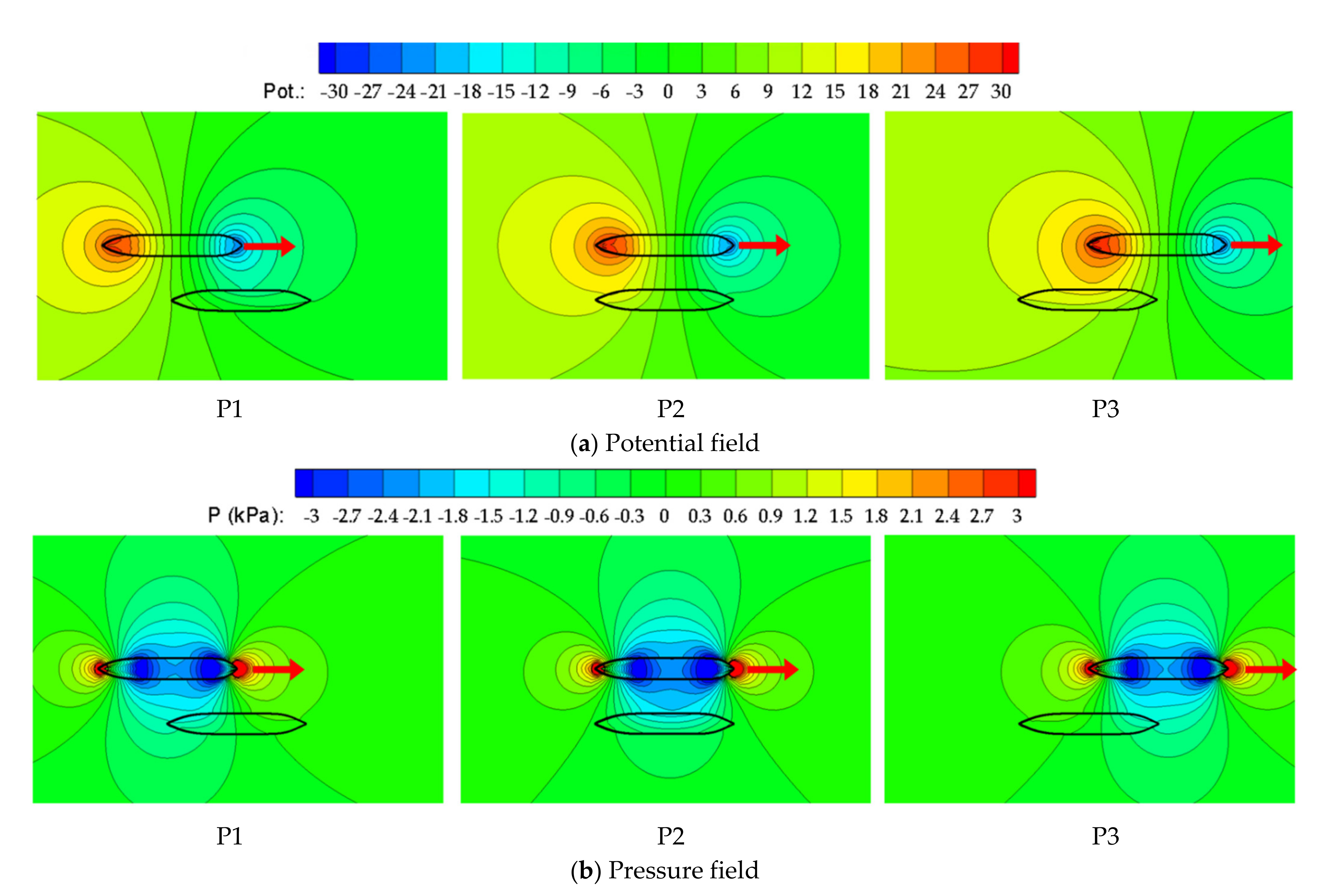
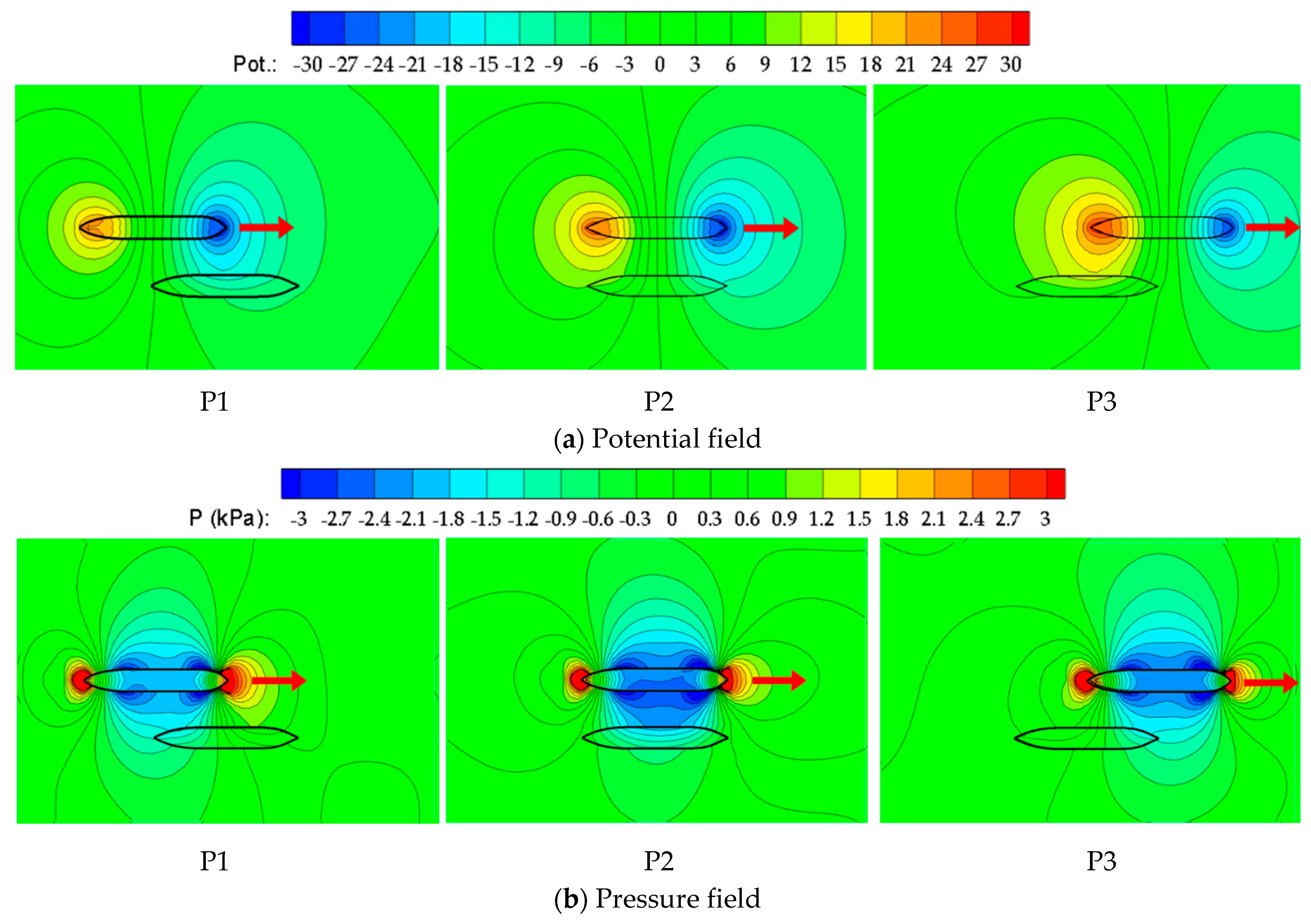
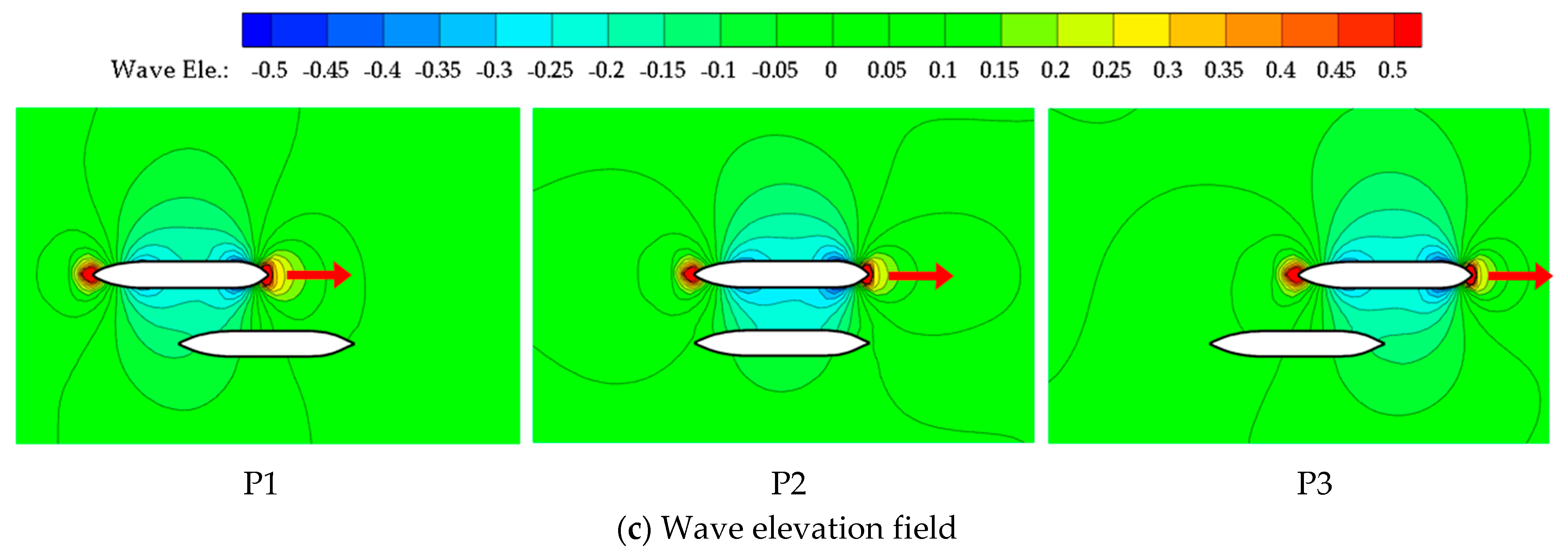
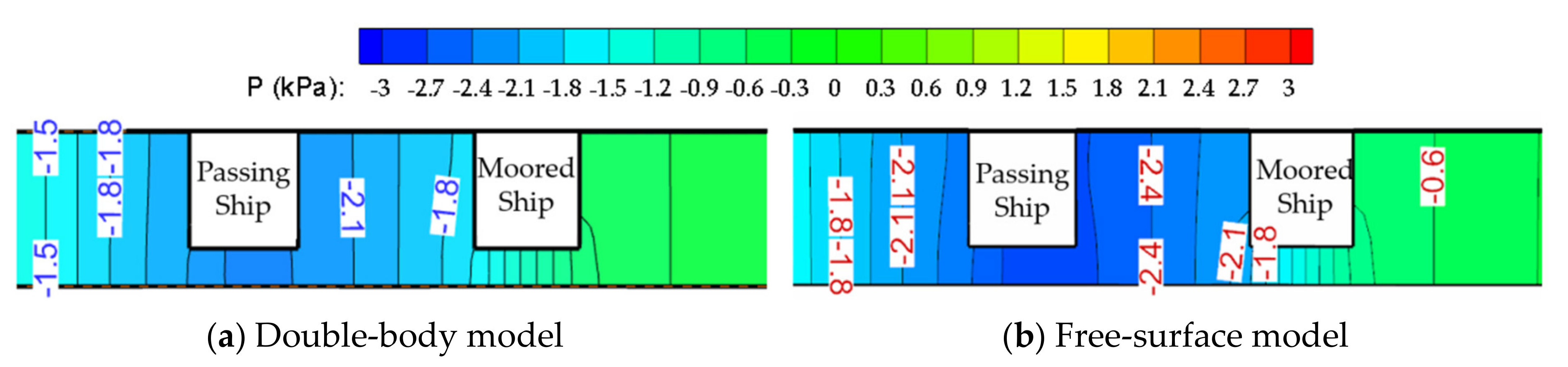
3.1. Double-Body vs. Free-Surface Models
3.2. Effects of Separation Distance and Water Depth
3.3. Effect of Ship Size
4. Conclusions
- -
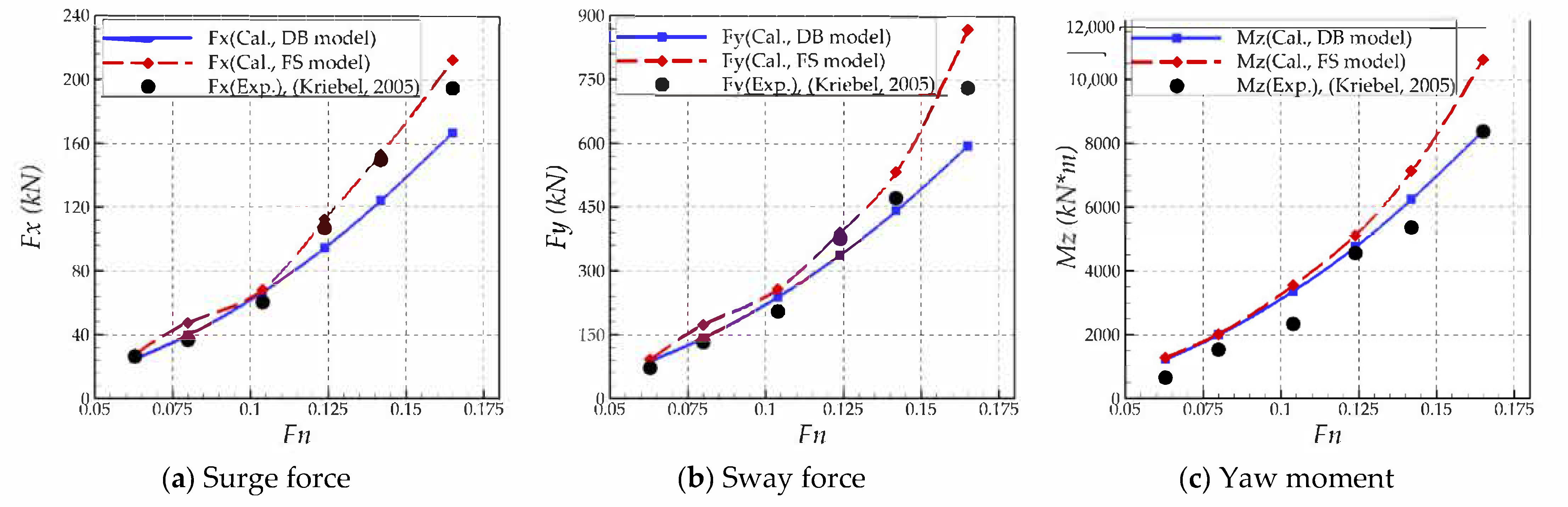
- The hydrodynamic forces and moment acting on the moored ship increase significantly as the speed of the passing ship increases. In particular, the passing ship load increases in proportion to the square of the passing ship speed under low Froude numbers less than 0.12, for which both the DB and FS models can accurately predict the passing ship loads. However, when the Froude number exceeds this limit, the passing ship load increases at a rate faster than the square of the passing ship speed, mainly due to the free-surface effect. Under this condition, it was found that the numerical results based on the FS model were closer to the model test data than those based on the DB model.
- -
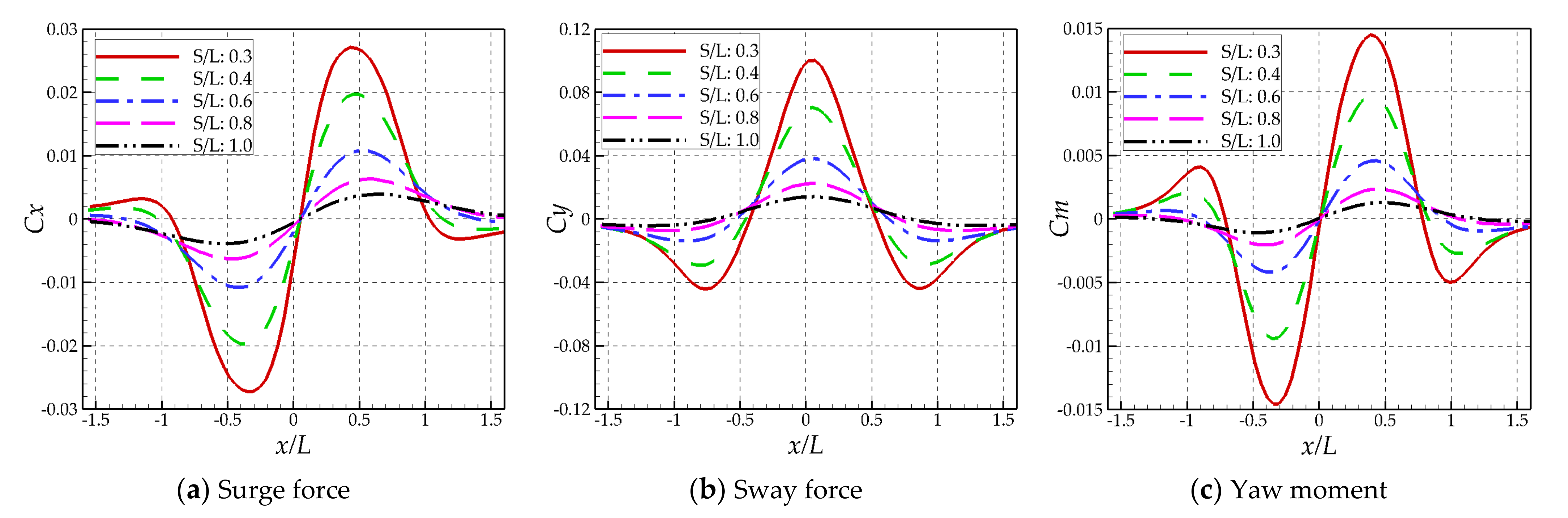
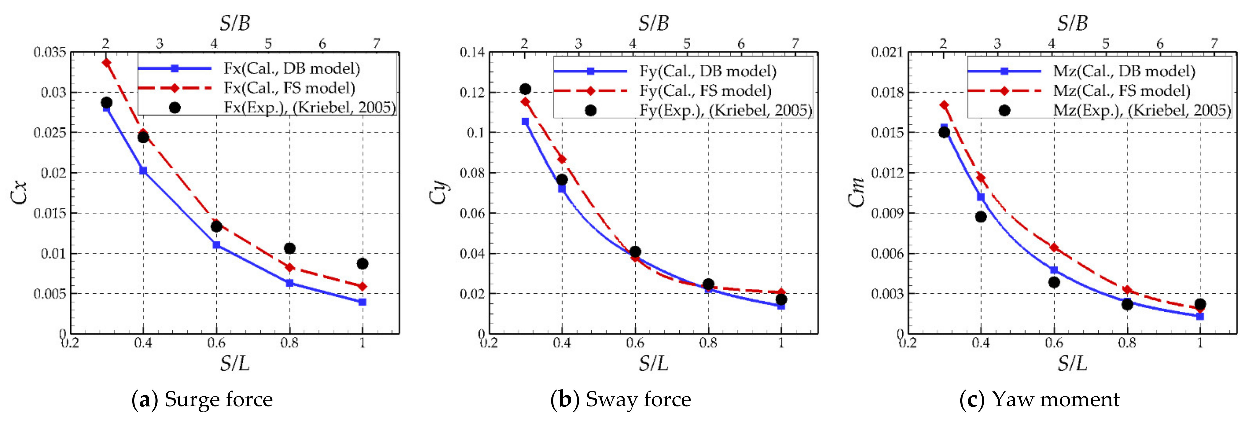
- The passing ship loads increase gradually with decreasing separation distance between the passing and moored ships. From the present numerical computations, it can be observed that the passing ship loads sharply increase when the separation distance ratio (S/B) becomes less than 4. Under low-speed conditions, the present numerical methods could predict the peak values of the passing ship loads with an error less than 10%, regardless of the separation distance.
- -
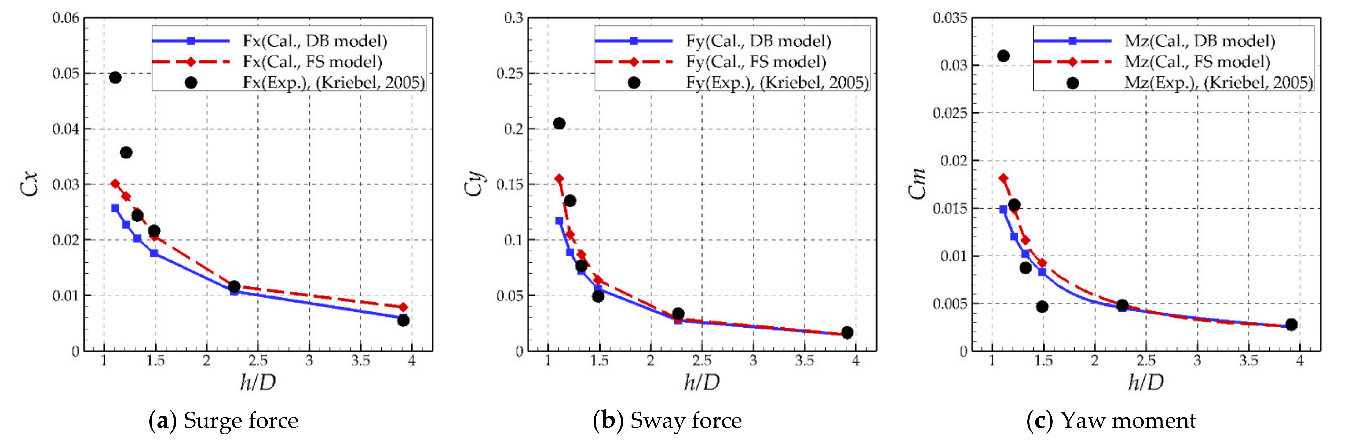
- As the water depth decreases, the passing ship load also increases. Especially under shallow water-depth conditions where the depth ratio (h/D) < 1.2, it could be clearly observed that the passing ship loads significantly increased.
- -
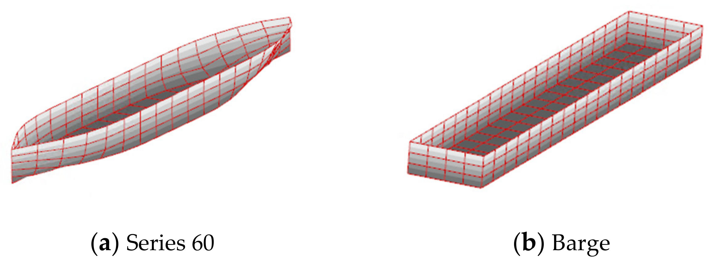
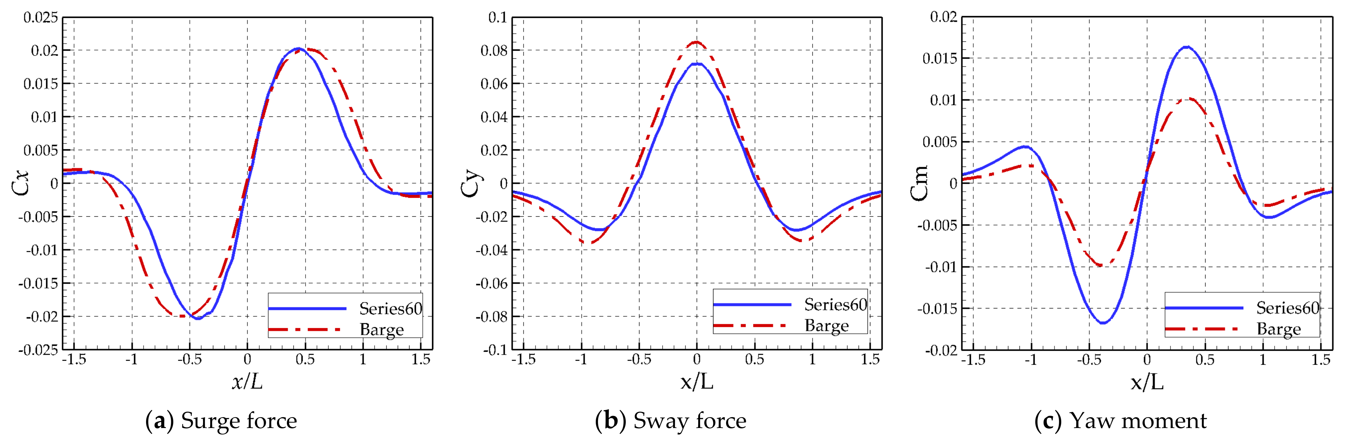
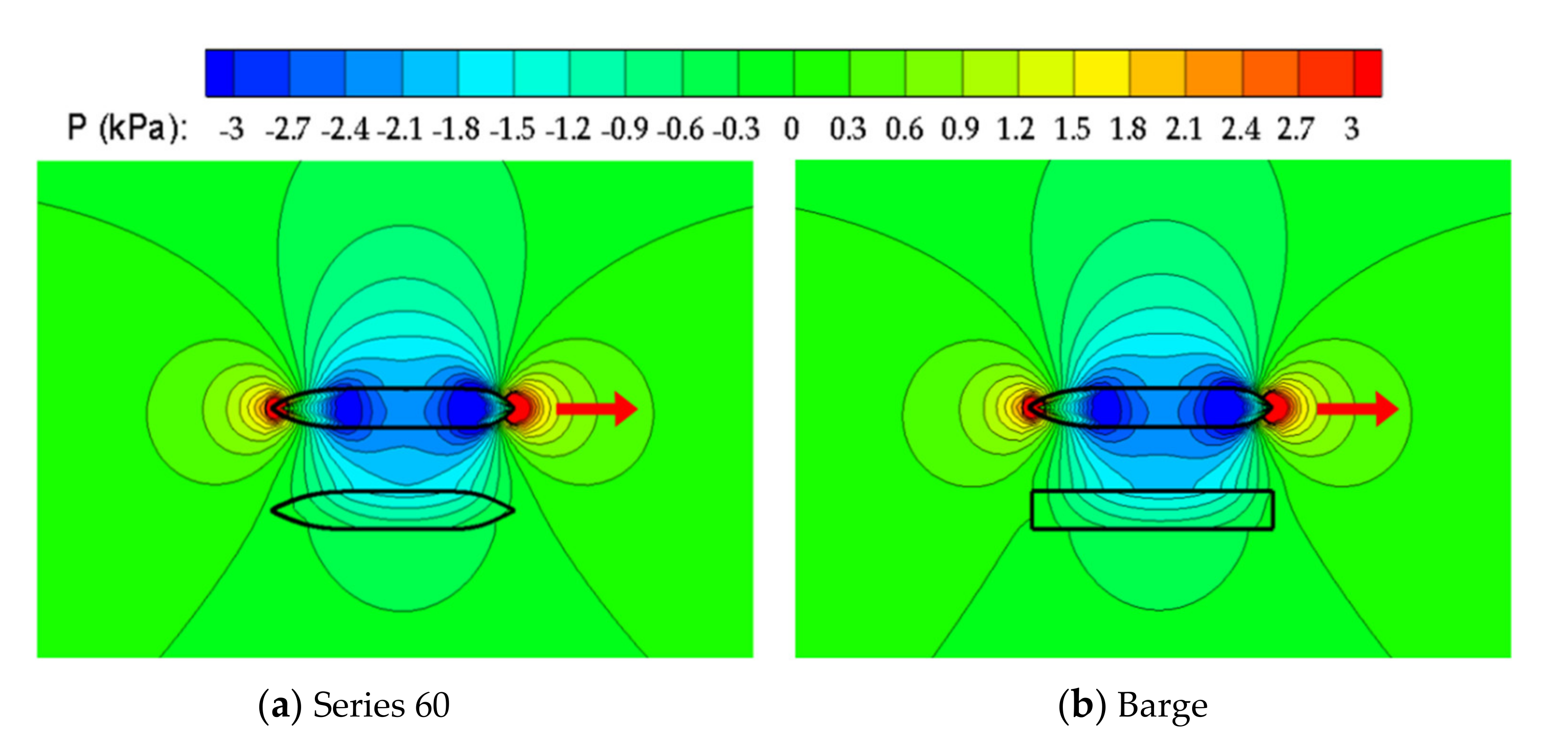
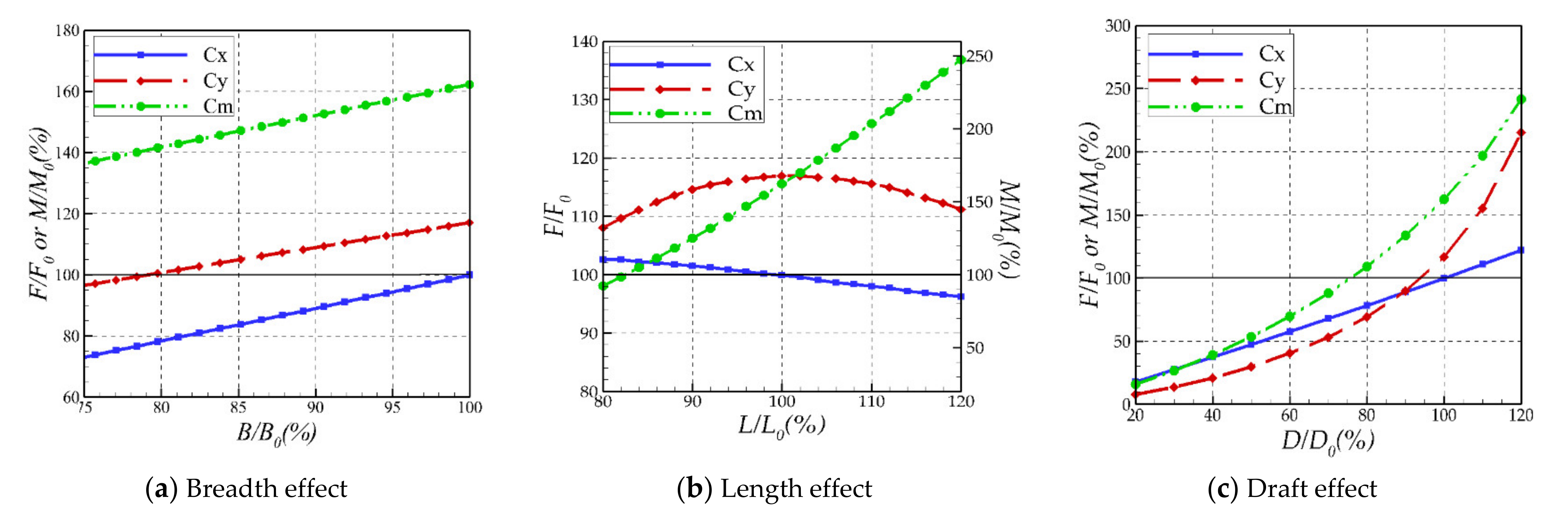
- The relative sizes of the moored and passing ships are a critical factor in the passing ship loads due to changing pressure fields formed around the moored ship. All the forces and moment increase linearly with increasing moored ship breadth. Furthermore, with an increase in the moored ship length, the surge force linearly decreases, and the yaw moment linearly increases. Compared to the changes in the breadth and length, passing ship loads are more sensitive to the change of the ship draft.
- -
- In the future, new validation data from model tests are required for a close examination of the free-surface effect in the passing ship problem. In addition, numerical studies on various ships should be performed by applying the developed numerical methods.
Author Contributions
Funding
Institutional Review Board Statement
Informed Consent Statement
Data Availability Statement
Acknowledgments
Conflicts of Interest
References
- National Transportation Safety Board (NTSB). Fire and Explosion Aboard the U.S. Tankship Jupiter; U.S. Depterment of Transportation: Bay City, MI, USA, 1990.
- Remery, G.F.M. Mooring forces induced by passing ships. In Proceedings of the Offshore Technology Conference, Dallas, TX, USA, 6–8 May 1974. [Google Scholar]
- Muga, B.; Fang, S. Passing Ship Effects–From Theory and Experiment. In Proceedings of the Offshore Technology Conference, Houston, TX, USA, 5–8 May 1975. [Google Scholar]
- Vantorre, M.; Verzhbitskaya, E.; Laforce, E. Model test based formulations of ship-ship interaction forces. Ship Tech. Res. 2002, 49, 124–141. [Google Scholar]
- Kriebel, D. Mooring Loads due to Parallel Passing Ships; Technical Report; TR-6056-OCN; Naval Facilities Engineering Service Center: Port Hueneme, CA, USA, 2005. [Google Scholar]
- Flory, J.F. The Effect of Passing Ships on Moored Ships. In Proceedings of the Prevention First 2002 Symposium, California State Lands Commission, Long Beach, CA, USA, 10–22 September 2002. [Google Scholar]
- Seelig, W.N. Passing Ship Effects on Moored Ships; Technical Report; TR-6027-OCN; Naval Facilities Engineering Service Center: Port Hueneme, CA, USA, 2001. [Google Scholar]
- Swiegers, P.B. Calculation of the Forces on a Moored Ship due to a Passing Container Ship. Ph.D. Thesis, Stellenbosch University, Stellenbosch, South Africa, 2011. [Google Scholar]
- Wang, S. Dynamic effects of ship passage on moored vessels. J. Waterw. Harb. Coast. Div. Am. Soc. Civ. Eng. 1975, 101, 247–258. [Google Scholar]
- Pinkster, J.A. The influence of a free surface of passing ship effects. Int. Shipbuild. Progr. 2004, 51, 313–338. [Google Scholar]
- Van der Molen, W.; Rossouw, M.; Phelp, D.; Tulsi, K.; Terblanche, L. Innovative technologies to accurately model waves and moored ship motions. In Proceedings of the Science Real and Relevant Conference, Stellenbosch, South Africa, 30 August–1 September 2010. [Google Scholar]
- Nam, B.W.; Park, J.Y. Numerical simulation for a passing ship and a moored barge alongside quay. Int. J. Nav. Archit. Ocean Eng. 2018, 10, 566–582. [Google Scholar] [CrossRef]
- Park, J.Y.; Nam, B.W.; Kim, Y.H. Prediction of hydrodynamic forces on passing ships. In Proceedings of the International Workshop on Water Waves and Floating Bodies (IWWWFB), Virtual Workshop, 24–27 August 2020. [Google Scholar]
- Huang, E.T.; Chen, H.C. Influences of ship specifics on passing ship effects. In Proceedings of the Sixteenth International Offshore and Polar Engineering Conference, Lisbon, Portugal, 1–6 July 2007. [Google Scholar]
- Wang, H.Z.; Zou, Z.J. Numerical study on hydrodynamic interaction between a berthed ship and a ship passing through a lock. Ocean. Eng. 2014, 88, 409–425. [Google Scholar] [CrossRef]
- Korsmeyer, F.T.; Lee, C.H.; Newman, J.N. Computation of Ship Interaction Forces in Restricted Waters. J. Ship Res. 1993, 37, 298–306. [Google Scholar] [CrossRef]
- Pinkster, J.A.; Ruijter, M.N. The Influence of Passing Ships on Ships Moored in Restricted Waters. In Proceedings of the Offshore Technology Conference, Houston, TX, USA, 3–6 May 2004. [Google Scholar]
- Pinkster, J.A. Suction, Seiche and Wash Effects of Passing Ships in Ports; PMH B.V.: Rotterdam, The Netherlands, 2009. [Google Scholar]
- Pinkster, J.A. Progress on Real-Time Prediction of Ship-Ship-Shore Interactions Based on Potential Flow. In Proceedings of the 4th International Conference on Ship Manoeuvring in Shallow and Confined Water, Hamburg, Germany, 23–25 May 2016; pp. 157–167. [Google Scholar]
- Todd, F.H. Series 60 Methodical Experiments with Models of Single-Screw Merchant Ships; Technical Report 1712; David Taylor Model Basin: Bethesda, MD, USA, 1963. [Google Scholar]
- Kriebel, D.; Seelig, W.; Judge, C. Development of a Unified Description of Ship-Generated Waves. In Proceedings of the U.S. Section PIANC Annual Meeting, Roundtable, and Technical Workshops, PIANC USA, Alexandria, VA, USA, 30 June 2003. [Google Scholar]


| Variable | FL | S/L | h/D | Moored Ship |
|---|---|---|---|---|
| Representative | 0.142 | 0.4 | 1.324 | Series 60 |
| Number of cases | 6 | 5 | 6 | 2 |
| Range | 0.063–0.163 | 0.3–1.0 | 1.108–3.919 | Series 60/Barge |
| (a) Froude Number | ||
|---|---|---|
| No. | FL | Fh |
| 1 | 0.063 | 0.222 |
| 2 | 0.080 | 0.281 |
| 3 | 0.104 | 0.365 |
| 4 | 0.124 | 0.435 |
| 5 | 0.142 | 0.498 |
| 6 | 0.165 | 0.578 |
| (b) Separation Distance | ||
| No. | S/L | S/B |
| 1 | 0.30 | 2.02 |
| 2 | 0.40 | 2.70 |
| 3 | 0.60 | 4.05 |
| 4 | 0.80 | 5.39 |
| 5 | 1.00 | 6.74 |
| (c) Water Depth | ||
| No. | h/D | D/h |
| 1 | 1.108 | 0.902 |
| 2 | 1.216 | 0.822 |
| 3 | 1.324 | 0.755 |
| 4 | 1.486 | 0.673 |
| 5 | 2.270 | 0.440 |
| 6 | 3.919 | 0.255 |
| Passing Ship | Moored Ship 1 | Moored Ship 2 | |
|---|---|---|---|
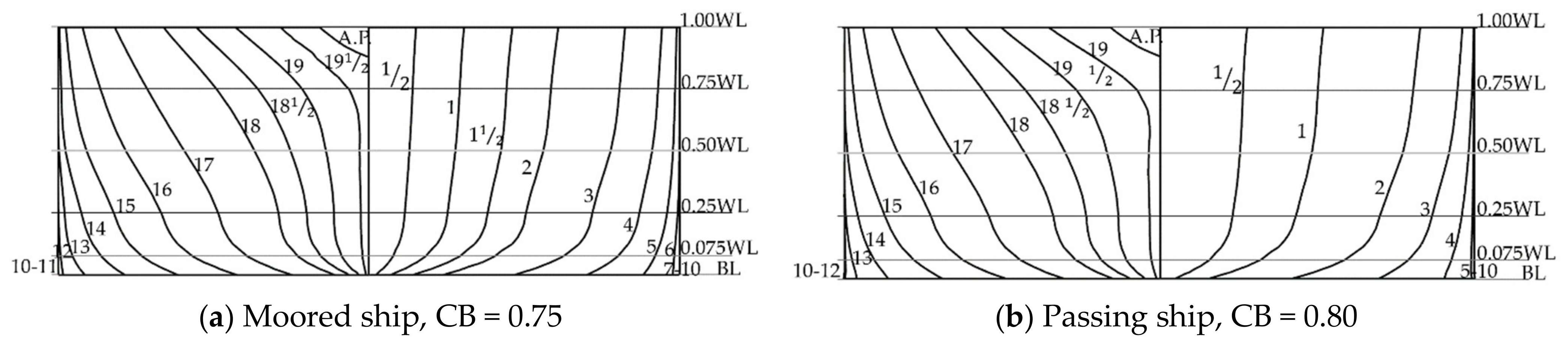
| Hull | Series 60, CB = 0.80 | Series 60, CB = 0.75 | Barge |
| Length(m) | 100 | 100 | 100 |
| Breadth(m) | 15.33 | 14.83 | 14.83 |
| Draft(m) | 6.17 | 6.17 | 6.17 |
Publisher’s Note: MDPI stays neutral with regard to jurisdictional claims in published maps and institutional affiliations. |
© 2021 by the authors. Licensee MDPI, Basel, Switzerland. This article is an open access article distributed under the terms and conditions of the Creative Commons Attribution (CC BY) license (http://creativecommons.org/licenses/by/4.0/).
Share and Cite
Park, J.-Y.; Nam, B.W.; Kim, Y. Numerical Analysis of Hydrodynamic Loads on Passing and Moored Ships in Shallow Water. Processes 2021, 9, 558. https://doi.org/10.3390/pr9030558
Park J-Y, Nam BW, Kim Y. Numerical Analysis of Hydrodynamic Loads on Passing and Moored Ships in Shallow Water. Processes. 2021; 9(3):558. https://doi.org/10.3390/pr9030558
Chicago/Turabian StylePark, Ji-Yong, Bo Woo Nam, and Yonghwan Kim. 2021. "Numerical Analysis of Hydrodynamic Loads on Passing and Moored Ships in Shallow Water" Processes 9, no. 3: 558. https://doi.org/10.3390/pr9030558