A Novel Prediction Process of the Remaining Useful Life of Electric Vehicle Battery Using Real-World Data

Abstract

In modern society, environmental sustainability is always a top priority, and thus electric vehicles (EVs) equipped with lithium-ion batteries are becoming more and more popular. As a key component of EVs, the remaining useful life of battery directly affects the demand of the EV supply chain. Accurate prediction of the remaining useful life (RUL) benefits not only EV users but also the battery inventory management. There are many existing methods to predict RUL based on state of health (SOH), but few of them are suitable for real-world data. There are several difficulties: (1) battery capacity is not easy to obtain in the real world; (2) most of these methods use the individual data for each battery, and the computing processes are difficult to perform in the cloud; (3) there is a lack of approaches for real-time SOH estimating and RUL predicting. This paper adopts several statistical methods to perform the prediction and compars the results of different models on experimental data (NASA dataset). Then, real-world data were implemented for an online process of RUL prediction. The main finding of this research is that the required CPU time was short enough to meet the daily usage after the real-world data was implemented for an online process of RUL prediction. The feasibility and precision of the prediction model can help to support the frequency control in power systems.

1. Introduction

Rechargeable lithium-ion batteries have been widely used in applications ranging from portable electronics to EVs in modern life due to their many advantages, such as their high volumetric and gravimetric energy density and low self-discharge rate [1]. Therefore, the growth of the EV market has been very rapid.

The safety and reliability of EVs compared to those of traditional vehicles are the top concerns of EV users. However, both safety and reliability are subject to not only the battery technology but also the management system for the battery [2]. The battery management system (BMS) has become one of the chief components in EVs. It provides the capability to monitor the working status of the battery and maintain all the cells within their operating limits. In particular, a BMS is expected to provide information about the three critical characteristics of a battery, namely the state of charge (SOC), the state of health (SOH), and the remaining useful life (RUL) [3].

The SOC is a measure of the remaining capacity of the battery. Due to the inherent chemical reactions of a battery, it is difficult to obtain a fully accurate value. There are two approaches to determining the SOC. The first is the direct approach, such as coulomb counting, which simply measures the remaining capacity by using the current integration [4]. On the other hand, indirect methods usually investigate the relationship between the SOC and some other electrical parameters such as open-circuit voltage (OCV) and impedance [5].

Traditional approaches to battery health management have mostly focused on SOC problems. However, in recent years, attention has increasingly been paid to the SOH and RUL. The SOH is a measure of a battery’s capability to deliver its specified output. Unlike the SOC, there is no clear-cut definition of the SOH [2].

The RUL refers to the available service time left before a system degrades to an unacceptable level [6], which is the EOL of the battery. It has also been suggested that when using an EV battery, an indicator $SO{H}_{EOL}$ is 0% when the battery capacity decreases to a certain level (70% or 80% of the nominal capacity is often considered to be the failure threshold) [7]. Below is the equation.

$$SO{H}_{EOL}=\frac{Q_{act}-Q_{threshold}}{Q_R-Q_{threshold}}\times 100\%$$

(1)

where $Q_R$ is the rated capacity and $Q_{act}$ is the actual capacity of the battery that is degraded. $Q_{threshold}$ is the capacity of the failure threshold. Therefore, the RUL indicates the remaining time or the number of load cycles until the battery reaches an $SO{H}_{EOL}$ of 0%.

A general definition of SOH is that it reflects the performance of a battery relative to its fresh condition. Therefore, the SOH is defined as 100% for a fresh cell and 0% for a cell that has reached the limitations of the end of life (EOL) [8]. Typically, the following equation in percentage form is used:

$$SOH=\frac{Q_{act}}{Q_R}\times 100\%$$

(2)

We note that the capacity, which quantifies the available energy stored in a fully charged Li-ion battery cell, is the indicator used most frequently to measure the SOH. However, it is not the only one. For example, Zhou et al. [9] proposed a novel health indicator that is formed by a series of battery discharging voltages.

Most previous works in RUL prediction used Equation (2) to measure SOH such as the NASA dataset we use in the following sections. We therefore use Equation (2) in this paper and employ a failure threshold of 70%.

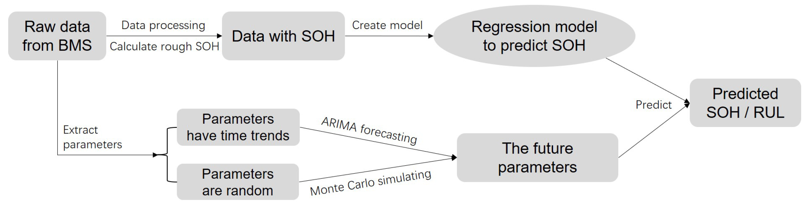
Figure 1 shows the relationship between the critical characteristics of a battery. The raw data from BMSs can be used to estimate the parameters or create models for specific purposes. Various studies focus on estimating the capacity and use it to estimate the SOC and SOH. When the SOH is determined, there are many methods of computing the probability density function (PDF) of the EOL so that the RUL can be predicted. Moreover, this paper introduces some real-world parameters such as driving behavior and environmental information that supplement SOH estimation and RUL prediction.

Barré et al. [10] divided the existing models for battery RUL prediction into five types: (1) electrochemical models, (2) equivalent circuit-based models, (3) performance-based models, (4) analytical models with empirical fitting, and (5) statistical approaches. Zhao et al. [11] simplified them into three parts: (1) electrochemical models, which need to use physical equations and are usually complex; (2) equivalent circuit-based models, such as particle filtering (PF) and other filtering methods; and (3) statistical models, which use data-driven methods without needing any prior knowledge about the battery aging mechanisms.

It is difficult to use physical equations and electrochemical reactions to obtain a reliable model. Most recent studies have focused on the last two types, namely model-based methods and data-driven methods. Model-based methods can be divided into two types: empirical equations and electrochemical principles [12]. Data-driven methods can be divided into two categories according to type of data. One is direct condition monitoring data, which are the data that can describe the underlying state of the system directly. We can use regression-based models, Wiener processes, gamma processes, and Markovian-based models to deal with them. On the other hand, for models based on indirect condition monitoring data, we include stochastic filtering-based models, covariate-based hazard models, hidden Markov models (HMMs), and hidden semi-Markov models (HSMMs) [13].

Zheng and Fang [14] indicated that the approaches that are purely model-based filtering and those that are purely data-driven have their respective limitations. They proposed hybrid approaches that incorporate model-based filtering approaches and data-driven approaches and classified them into three types: (1) models that compensate for the physical state/measurement model, (2) approaches to predict future trends in measurement values, and (3) methods to estimate the model parameters for the physical-based methods to predict.

Rather than data-driven methods, the model-based filtering techniques that feature closed-loop expressions can self-correct and overcome unexpected disturbances [15]. A Kalman filter–based prognostic method was developed to predict the battery RUL in 2009 [16]. Dong et al. [17] improved the standard particle filter and developed an SVR-PF that introduced novel capacity degradation parameters to determine the battery health in real time in 2014. Zhang et al. [18] proposed an improved unscented particle filtering (IUPF) method for lithium-ion battery RUL prediction based on the Markov chain Monte Carlo (MCMC) method in 2017. Duong and Raghavan [19] introduced a Heuristic Kalman algorithm in 2018, a metaheuristic optimization approach, that was combined with particle filtering to tackle sample degeneracy. Zhang et al. [20] presented an improved PF algorithm in 2018 based on linear optimizing combination resampling (U-LOCR-PF) to improve prediction accuracy. Ma et al. [21] developed a Gauss–Hermite particle filter (GHPF) to update the parameters of the capacity degradation model in real time and predict the RUL in 2019. Li et al. [22] developed an inheritance PF by using the genetic algorithm framework in 2019.

Data-driven methods can capture the inherent relationships and learn the trends present in the data to provide RUL predictions. They do not require specific knowledge of material properties, constructions, or failure mechanisms, and they do not involve the development of high-level physical models of the system; therefore, they have become increasingly popular for Li-ion battery RUL prediction [23]. Ng et al. [24] proposed a naive Bayes (NB) model for the RUL prediction of batteries under different operating conditions in 2014. Patil et al. [25] transformed the RUL into a classification problem in 2015 so that some machine learning methods could be used to estimate the RUL level. Zhou and Huang [26] proposed a novel approach that combines empirical mode decomposition (EMD) and the autoregressive integrated moving average (ARIMA) model in 2016. Zhang et al. [27] developed an RUL-prediction method in 2019 based on the Box–Cox transformation (BCT) and Monte Carlo (MC) simulation.

In recent years, deep learning has become very popular in all fields. Wu et al. [28] investigated the relationship between the RUL and the charge curve and simulated it in 2016 using a feed-forward neural network (FFNN) due to its simplicity and effectiveness. Zhang et al. [29] employed the long short-term memory (LSTM) recurrent neural network (RNN) in 2018 to learn the long-term dependencies among the degraded capacities of lithium-ion batteries. Khumprom and Yodo [30] presented a deep neural network (DNN) approach in 2019 to predict the SOH and the RUL.

In addition to the general parameters extracted from monitoring data, some other methods deserve attention. Chen et al. [31] presented a geometrical approach to Li-ion battery capacity estimation in 2014. They utilized four geometrical features that are sensitive to slight changes and degradation in performance. Wang et al. [32] found that different discharge rates (DDRs) affect both usable battery capacity and battery degradation rates. They designed an experiment to collect accelerated battery life testing data for DDRs in 2017, which were used to investigate how DDRs influence usable battery capacity.

Besides the aging of batteries, calendar aging (i.e., aging at rest) is also very important since parking time can reach 90% of the total vehicle lifetime. Eddahech et al. [33] presented a method for the calendar aging quantification of power batteries taking into account the SOC and temperature effects.

In the real world, the relation between battery parameters and the RUL is more complicated. The condition of a Li-ion battery is affected by the road conditions, environmental temperatures, charge modes, and even the driver’s behavior. Nuhic et al. [34] used real-word data to estimate SOH and RUL but lack applicable data and thus are based on uniform tests. Canals et al. [35] extracted temperature, voltage, current, and energy exchanges data from on-board data-loggers installed in an EV and calculated the internal resistance and voltage recovery, so that the SOH can be estimated.

However, few of them are suitable for real-world data. There are several difficulties: (1) battery capacity is not easy to obtain in the real world; (2) most of these methods use individual data for each battery, and the computing processes are difficult perform in the cloud; (3) there is a lack of approaches for real-time SOH estimating and RUL prediction.

Many studies mentioned above focused on creating models for batteries separately. Indeed, these are accurate approaches if data are sufficient. Most automobiles do not have enough computing power to improve computing speed and save resources. This paper proposes to create an aggregated model for all of the vehicle data and use personalization parameters to reflect the individual characteristics.

This paper attempts to introduce more influencing factors for RUL prediction based on real-world data and proposes an online data-driven approach to rapidly estimating the SOH and RUL. The required CPU time was short enough to meet the daily usage after the real-world data were implemented for an online process of RUL prediction. Alhelou et al. [36] discussed the contribution of EVs in supporting the frequency control in power systems, and the feasibility and precision of the RUL prediction model of EVs can help to overcome the uncertainties of the electric demands.

2. Materials and Methods

2.1. Overview

Figure 2 shows the process structure of RUL prediction based on real-world data. The raw data usually come from a BMS and do not contain accurate SOH value, so we need to calculate rough SOH at first and then create a statistical model using real-world parameters. When we successfully forecast or simulate the future parameters, this statistical model could be used to predict the future SOH and RUL.

In this study, we first use the NASA Ames Li-ion battery cycle life test data [37] since they contain accurate capacity values, allowing us to train precise models and compare the methods. Figure 3 shows the process using NASA data.

2.2. Introduction to NASA Dataset

There are four Li-ion batteries (#5, #6, #7, and #18), which were run through 3 different operational profiles (charge, discharge, and impedance) at room temperature. Charging was carried out in constant current (CC) mode at 1.5 A until the battery voltage reached 4.2 V and then continued in a constant voltage (CV) mode until the charge current dropped to 20 mA. Discharge was carried out at a constant current (CC) level of 2 A until the battery voltage fell to 2.7 V, 2.5 V, 2.2 V, and 2.5 V for batteries #5, #6, #7, and #18, respectively. The experiments were stopped when the batteries reached the EOL criterion, which was a 30% fade in rated capacity (from 2 Ahr to 1.4 Ahr). Figure 4 shows the relationship between the capacity and cycle number. The number of cycles are 168, 168, 168, 132, for batteries #5, #6, #7, and #18.

According to Equation (2), we can compute the SOH value at each point, and the results are shown in Figure 5.

Table 1. Sample of NASA dataset.

Type	Time_Start	Time_End	Capacity	${\mathit{v}}_1$	⋯	${\mathit{i}}_1$	⋯	${\mathit{t}}_1$	⋯
charge	2008/4/2 13:08	2008/4/2 15:14		4.187		0.643		25.32
discharge	2008/4/2 15:25	2008/4/2 16:27	1.856487	3.530		−1.819		32.57
charge	2008/4/2 16:37	2008/4/2 19:33		4.059		0.949		26.64
discharge	2008/4/2 19:43	2008/4/2 20:45	1.846327	3.537		−1.818		32.73
charge	2008/4/2 20:55	2008/4/2 23:50		4.058		0.951		26.78
discharge	2008/4/3 0:01	2008/4/3 1:01	1.835349	3.544		−1.816		32.64

shows some sample records of NASA dataset.

$v_i$, $i_i$, and $t_i$ mean the voltage, output current, and temperature of a battery at the i-th time point, respectively.

2.3. SOH Estimation

The NASA dataset contains an accurate capacity in each discharge cycle; therefore, we can calculate the accurate SOH and use it as the response variable. We extracted some features from the internal battery parameters (voltage, output current, and temperature) in each discharge cycle.

Table 2. Variables in each discharge cycle.

Variable	Description	Variable	Description
soh	SOH in each discharge cycle	imin	minimum of output current
cycle	cycle number	iavg	average of output current
tambient	ambient temperature	isd	standard deviation of output current
vmax	maximum of voltage	tmax	maximum of temperature
vmin	minimum of voltage	tmin	minimum of temperature
vavg	average of voltage	tavg	average of temperature
vsd	standard deviation of voltage	tsd	standard deviation of temperature
imax	maximum of output current

shows the variables in the dataset. There is only one real-world parameter: ambient temperature. In this dataset, the ambient temperature remains unchanged, so it will not be selected in the final models.

We will try some regression models to predict SOH. The voltage, output current, and temperature measurements in each discharge cycle were selected as independent variables. To obtain more features, we conducted feature engineering by extracting the maximum, minimum, mean, and standard deviation from all of the measurements. We defined these 3 models according to different data scenarios.

• Model 1: Use the individual data for each battery to predict that battery’s SOH.
• Model 2: Use all of the data to create an aggregate model to predict each battery.
• Model 3: Use the data for the other batteries to predict the SOH for another battery. For example, we combine the data for batteries #5, #6, and #7 to predict battery #18.

Linear regression is the simplest model, but there may be correlation and linear dependence between explanatory variables. We will also therefore try Lasso and ridge regression.

The Lasso [38] (least absolute shrinkage and selection operator) is a regression with an ${\ell }_1$-norm penalty, which minimizes the residual sum of squares subject to the sum of the absolute value. Because of its good performance in both variable selection and prediction accuracy, Lasso is popular for predicting continuous variables. Mansouri et al. [39] discussed how to use Lasso to predict the RUL of a battery. To improve computing efficiency, Friedman et al. [40] developed fast algorithms to estimate generalized linear models with convex penalties.

A general form of the Lasso is elastic net. Suppose that we have observations $x_i\in {\mathbb{R}}^p$ and the responses $y_i\in \mathbb{R},i=1,\dots ,N$. The objective function is

$$\underset{({\beta }_0,\beta )\in {\mathbb{R}}^{p+1}}{\min }\frac{1}{2N}\sum _{i=1}^N{(y_i-{\beta }_0-x_i^T\beta )}^2+\lambda \left[{(1-\alpha )\left|\right|\beta \left|\right|}_2^2/2+{\alpha \left|\right|\beta \left|\right|}_1\right],$$

(3)

where $\lambda \ge 0$ is a complexity parameter and $0\le \alpha \le 1$ is a compromise between the ${\ell }_1$-norm and ${\ell }_2$-norm. $\alpha =0$ means the ridge regression, and $\alpha =1$ means the Lasso. The elastic net is a regularized regression method that linearly combines the ${\ell }_1$-norm and ${\ell }_2$-norm penalties of the Lasso and ridge methods.

We use the root mean square error (RMSE) to compare the performance of the methods:

$$RMSE=\sqrt{\sum _{k=1}^m{({\widehat{SOH}}_k-SO{H}_k)}^2/m}$$

(4)

where $SO{H}_k$ is the $SOH$ value at cycle number k, and $\widehat{SOH}$ represents the predicted value.

This approach is based on the internal battery parameters and predicts the current SOH value. It cannot be directly used to predict the future SOH and thus predict the RUL. Although there are many methods to estimate the SOH and predict the RUL at the same time, these methods usually have high requirements for data and have time-consuming calculation processes. In the real world, there are often missing values, and batteries are seldom fully discharged. Using this approach, we need only the internal battery parameters and other parameters of the current state to estimate the value of the current SOH, which is meaningful for the residual value evaluation of the battery. In addition, the calculation process is both simple and fast, which is suitable for real-time computing on the cloud. Finally, the estimated SOH value can be combined with other methods, such as ARIMA, to predict the RUL.

2.4. RUL Prediction

2.4.1. RUL Prediction by Using Time Series Method Directly

A time series is a set of observations $x_t$, each one being recorded at a specified time t [41]. Time series forecasting involves using existing data to make predictions about future events. The autoregressive integrated moving average (ARIMA) method is a popular model to identify complex patterns in data and to generate forecasts [42].

Hyndman and Khandakar [43] developed a step-wise algorithm for automatic forecasting with ARIMA models. By using this algorithm, we can select the model that minimizes the Akaike’s information criterion (AIC) or Bayesian information criterion (BIC) among all of the models that are appropriate for the data.

The ARIMA method can be used to predict the RUL based on the historical data, and Zhou and Huang [26] have discussed the approaches to predict the battery RUL by forecasting the next step SOH.

If we obtain historical SOH series, we can apply the ARIMA model to predict the future SOH. First, we make the SOH prediction at 4 different starting points for each battery. For example, starting at point 60 means that we use data from cycle 1 to cycle 59 as the training dataset and then forecast the future values of the SOH. The RMSE is used as the evaluation criterion to evaluate the performance of SOH prediction.

2.4.2. RUL Prediction by the Regression Methods

When we use time series methods, a smaller number of data results in lower prediction accuracy. There is another strategy to determine the future parameters at first and then predict the SOH, which is using regression methods.

If the parameters have time trends, we can use the ARIMA model to predict the future values. If the parameters are random or unpredictable, such as driving behaviours, we can use a Monte Carlo simulation to determine the future values. Then, regression models can be used to predict the SOH.

If simulated data are used, we can obtain the PDF of the RUL. For the sake of simplicity, we use the ARIMA model to predict the internal battery parameters, and we then use the Lasso regression to predict the SOH and RUL.

2.5. Results

2.5.1. SOH Estimation by Regression Models

First, we employ a linear regression to predict the SOH for each battery. Figure 6 shows the prediction result of each model for each battery.

We find that most of the results are good, except for model 3 on batteries #6 and #18.

Using the same definition of the 3 models, we employ a ridge regression to predict the SOH. The results are shown in the Figure 7.

Model 3 on battery #5 seems to obtain better performance, but the others are not as good as the linear regression.

Then, we employed the Lasso regression. The results are shown in the Figure 8.

Model 3 on battery #6 seems to be a little bit better than the linear regression, and the others do not seem to be worse.

Table 3. RMSE (%) results of all the models.

Battery	Linear Regression			Ridge Regression			Lasso Regression
	Model 1	Model 2	Model 3	Model 1	Model 2	Model 3	Model 1	Model 2	Model 3
#5	0.4	0.93	1.04	0.91	1.42	1.6	0.41	0.94	1.02
#6	0.63	1.22	5.57	1.09	1.45	4.44	0.77	1.2	5.64
#7	0.39	0.84	1.87	0.85	1.68	3.78	0.41	0.88	1.98
#18	0.32	1.24	3.2	0.55	1.72	4.95	0.33	1.23	3.33

shows the RMSE results of each method used for each battery, and we find that the linear regression model is the best in most cases. To prevent overfitting, we mainly refer to model 3. We find that the ridge regression has the best prediction result for battery #6, but it has poor performance on the other batteries. The Lasso has similar performance as the linear regression.

2.5.2. RUL Prediction When SOH Is Determined

In this paper, we set 70% of the SOH as the failure threshold. Thus, we can predict the RUL by counting the remaining life (in number of cycles) before the battery reaches the EOL. The absolute error (AE) is used to evaluate the performance of RUL prediction. The RMSE of SOH is computed according to Equation (4). Since the SOH prediction before the EOL is more important, we also list the RMSE when $SOH>70\%$. The results are shown in Figure 9 and

Table 4. Prediction results of ARIMA.

Battery	Starting	ARIMA	Actual	Predicted	AE	RMSE of SOH %	RMSE of SOH %
	Point	(p, d, q)	RUL	RUL		(Overall)	(SOH > 70%)
#5	60	(0, 1, 0)	65	111	46	5.32	4.44
	70	(0, 1, 0)	55	70	15	2.09	2.00
	80	(0, 1, 0)	45	48	3	1.01	0.92
	90	(0, 1, 0)	35	30	5	1.99	1.34
#6	60	(0, 1, 0)	49	35	14	7.67	3.05
	70	(0, 1, 3)	39	21	18	9.58	4.28
	80	(0, 1, 3)	29	12	17	9.65	4.64
	90	(0, 1, 3)	19	4	15	9.05	4.80
#7	60	(0, 1, 0)	109	129	20	2.90	2.90
	70	(0, 1, 0)	99	88	11	0.99	0.99
	80	(0, 1, 0)	89	69	20	1.84	1.84
	90	(0, 1, 0)	79	55	24	2.47	2.47
#18	60	(0, 1, 3)	37	50	13	2.43	2.73
	70	(0, 1, 0)	27	19	8	5.09	1.61
	80	(2, 1, 3)	17	12	5	4.68	1.23
	90	(2, 1, 3)	7	5	2	4.04	0.67

.

Since the degradation of battery #7 does not reach the failure threshold, the RMSE of the overall data is the same as the RMSE of the data when $SOH>70\%$. For the other batteries, the predictions are better when $SOH>70\%$.

2.5.3. RUL Prediction When SOH Is Not Determined

In the real world, battery capacity is not easy to obtain, so there is no accurate SOH value available when we predict the RUL. A feasible way would be forecasting the battery parameters at first and then predicting the RUL by regression model.

Firstly, we forecast the future parameters listed in Table 2 by the ARIMA model. Then, we use Model 2 of Linear/Ridge/Lasso regression to predict RUL. After comparing the results, we choose the Ridge regression model. The results are shown in Figure 10 and

Table 5. Prediction results of regression models.

Battery	Starting	Actual	AE	AE	AE	RMSE %	RMSE %
	Point	RUL	(Linear)	(Lasso)	(Ridge)	(Overall)	(SOH > 70%)
#5	60	65	85	84	112	8.44	6.37
	70	55	29	28	9	1.42	1.53
	80	45	35	33	1	1.70	0.87
	90	35	22	21	8	3.23	1.38
#6	60	49	54	54	78	7.84	4.44
	70	39	29	28	15	5.45	3.26
	80	29	23	22	14	5.38	3.61
	90	19	7	6	14	6.57	4.46
#7	60	109	87	84	104	6.75	6.75
	70	99	50	49	27	2.62	2.62
	80	89	62	60	26	2.55	2.55
	90	79	52	51	29	3.26	3.26
#18	60	37	10	14	34	3.76	4.07
	70	27	10	10	18	1.99	2.25
	80	17	10	10	18	1.97	2.36
	90	7	4	4	12	1.83	1.70

.

We find that the predictions at starting point 60 are not good. Compared with the ARIMA model with determined SOH, this model has better prediction results for battery #5 and #6 at starting points 70/80/90, and the others do not seem too bad. So when we do not have accurate SOH value in the real world, we can use this process to predict the RUL.

3. Application Study with Data from the Real World

3.1. Data Description

Table 6. Sample of real world data.

$\mathit{vin}$	Time	Mode	$\mathit{soc}$	i	${\mathit{v}}_1$	⋯	${\mathit{t}}_1$	⋯	$\mathit{lon}$	$\mathit{lat}$	$\mathit{odomileage}$
test1	2016/9/22 20:29:01	2	61.6	1.64	3.28		25		0	0	192
test1	2016/9/22 20:29:11	1	61.6	0	3.28		25		0	0	192
test1	2016/9/23 01:31:01	1	61.6	0	3.28		25		0	0	192
test1	2016/9/26 06:15:01	4	61.6	−8.58	3.3		26		0	0	192
test1	2016/9/26 06:15:11	4	61.6	−8.58	3.3		26		121.446	31.218	192
test1	2016/9/26 06:15:21	4	61.6	−8.48	3.32		26		121.446	31.218	192

shows some sample records of real-world data from a BMS. Each record contains the status informations of an EV at a time point, such as cell voltage, cell temperature, charge mode, mileage, and a rough SOC value.

The variable $mode$ means charge mode; $soc$ means the rough SOC value; i means charge or discharge current; $v_k$ means voltage of the k-th battery cell; $t_k$ means temperature of the k-th battery cell; $lon$ means longitude; $lat$ means latitude; $odomileage$ means ODO mileage.

We need to estimate battery capacity based on these values to calculate the SOH. From time point $t_1$ (the start time of a discharge cycle) to $t_2$ (the end time of a discharge cycle), the total capacity of the battery cell is [44]:

$$C=C_{1,2}=\frac{Q_1-Q_2}{SO{C}_1-SO{C}_2}=\frac{{\int }_{t_1}^{t_2}I\left(t\right)dt}{SOC\left(t_1\right)-SOC\left(t_2\right)}$$

(5)

In the real world, the number of BMS data is huge: there are usually several records in 1 s. Sometimes there are errors in the data, which need to be cleaned.

The data come from a BMS that contains 363 vehicles samples. The data contain real-time current, voltage, temperature, and other information, as well as a rough estimate of the SOC.

We use Equation (5) to estimate the rough value of capacity and use it to compute the SOH value by following the Equation (2). Figure 11 shows the SOH details of all the vehicles. It is a smoothed color density representation of a scatterplot, obtained through a kernel density estimate. Dark area means high density of data points.

3.2. SOH Estimation

We found that the maximum number of cycles was only 300, and the batteries of these vehicles are far from the EOL; therefore, there is no way to obtain exact future SOH values. We can use the methods mentioned in the previous section to create models with the SOH and various battery parameters and then use these models to predict the future SOH. It should be noted that many vehicles do not contain enough data points, and there is a large number of vehicles in the real world; therefore, it is necessary to build an aggregate model to predict each vehicle.

As mentioned above, we continue to use the three models: the linear regression, the ridge regression, and the Lasso regression. For each method, we create an aggregate model (use all of the samples) and predict the vehicles separately.

Table 7. RMSE (%) results of all the models.

	Linear Regression	Ridge Regression	Lasso Regression
Mean of RMSE	0.92	0.93	0.92
Median of RMSE	0.6	0.62	0.61
Maximum of RMSE	8.56	8.6	8.56
Minimum of RMSE	0.08	0.08	0.08

shows the RMSE results.

We found that there is little difference between the results of these models. The Ridge regression obtained the best performance when we use NASA dataset, so we selected the Ridge regression for the subsequent prediction.

3.3. RUL Prediction

To predict the future SOH, we need the future battery parameters. In practice, we can use a Monte Carlo simulation to determine the PDF of the RUL. Without losing generality, we investigate the historical data of two features, the charge mode and mileage, for vehicle #1. Figure 12 shows their distributions.

We can use a binomial distribution to simulate charge mode and a log-normal distribution to simulate mileage per day. The parameters are shown in the

Table 8. Distribution parameters of the charge model and mileage per day for vehicle #1.

Feature	Distribution	Parameters
Charge mode	binomial	$n=1$, $p=0.284$
Mileage per day	log-normal	$\mu =3.482$, $\sigma =0.981$

.

Then, future data over a period of time can be simulated. We did multiple simulations and compute the PDF of the RUL. Figure 13 is the result of four simulation scenarios for vehicle #1; each scenario used a different random number seed.

Table 9. Simulation parameters for vehicle #1.

Scenario	Random Number Seed	Simulation Times	Maximum Cycles
1	1	100	5000
2	2	100	5000
3	3	100	5000
4	4	100	5000

shows the simulation parameters. Appendix A shows the R codes.

For example, in scenario 1, according to the peak value of the density estimation, the predicted EOL for vehicle #1 is the 1592th cycle. Since the last cycle number for prediction is 261, the RUL is 1331 cycles.

In the four simulation scenarios, the minimum of predicted EOL is 1584, the maximum of predicted EOL is 1602, the difference rate is 1.14%, and it shows that the simulated result is quite stable.

We have run 1000 simulations to compute the PDF, the total CPU time on a PC (AMD Ryzen 5 3500U) is 0.03 s. The computing performance can meet the daily needs.

3.4. Discussion

When we compute the SOH value of a EV, we can predict the short-term demand for electricity. When we compute the RUL of a EV, we can predict the long-term demand for electricity. The electric demands of EVs was taken account into basic load frequency control (LFC) of power systems. LFC in power systems can generate control signals and apply it to the governors to match supply and demand. There are lots of methods to improve the performance of LFCs by tuning them such as [45,46]. In order to handle the parametric and non-parametric uncertainties of realistic power systems, Alhelou et al. [47] devoloped a unknown input functional observer (UIFO) [47] or unknown input observer (UIO) [48] for LFC. The unknown input observer can also be used for fault detection and isolation [49]. If we can accurately predict the electric demands, we can provide more information for LFC.

4. Conclusions and Future Works

A novel process for predicting the RUL using real-world data was proposed. First, the SOC-based equation was used to estimate the capacity and SOH of the battery for each electric vehicle. Second, a Lasso regression model was constructed with the aggregated data for all the vehicles after missing and invalid values were removed. Then, the future internal battery parameters and real-world parameters were predicted by the ARIMA model or simulated by the Monte Carlo method. Finally, the future values of the SOH were predicted by the Lasso model with the predicted parameters, and the probability distribution of the RUL was determined.

This approach is less reliant on experimental data and can easily perform real-time prediction; therefore, it is economical to apply it to evaluate a vehicle’s condition and the residual value of the battery. It has significance for the battery recovery industry and thus has some contribution to the green supply chain of the automobile industry. Based on Section 3.4, we will use the RUL prediction model to predict the electric demands and make more improvement to the LFC of the power systems in future work.

References

1. Vetter, J.; Novák, P.; Wagner, M.R.; Veit, C.; Möller, K.C.; Besenhard, J.O.; Winter, M.; Wohlfahrt-Mehrens, M.; Vogler, C.; Hammouche, A. Ageing mechanisms in lithium-ion batteries. J. Power Sources 2005, 147, 269–281. [Google Scholar] [CrossRef]
2. Xing, Y.; Ma, E.W.M.; Tsui, K.L.; Pecht, M. Battery Management Systems in Electric and Hybrid Vehicles. Energies 2011, 4, 1840–1857. [Google Scholar] [CrossRef]
3. Pattipati, B.; Sankavaram, C.; Pattipati, K.R. System Identification and Estimation Framework for Pivotal Automotive Battery Management System Characteristics. IEEE Trans. Syst. Man Cybern. Part C 2011, 41, 869–884. [Google Scholar] [CrossRef]
4. Finger, E.P.; Marwell, E.M. Battery Control System for Battery Operated Vehicles. U.S. Patent 4,012,681, 1 September 1977. [Google Scholar]
5. Chiang, Y.H.; Sean, W.Y.; Ke, J.C. Online estimation of internal resistance and open-circuit voltage of lithium-ion batteries in electric vehicles. J. Power Sources 2011, 196, 3921–3932. [Google Scholar] [CrossRef]
6. Zhang, J.; Lee, J. A review on prognostics and health monitoring of Li-ion battery. J. Power Sources 2011, 196, 6007–6014. [Google Scholar] [CrossRef]
7. Waag, W.; Fleischer, C.; Sauer, D.U. Critical review of the methods for monitoring of lithium-ion batteries in electric and hybrid vehicles. J. Power Sources 2014, 258, 321–339. [Google Scholar] [CrossRef]
8. Wei, J.; Dong, G.; Chen, Z. Remaining Useful Life Prediction and State of Health Diagnosis for Lithium-Ion Batteries Using Particle Filter and Support Vector Regression. IEEE Trans. Ind. Electron. 2018, 65, 5634–5643. [Google Scholar] [CrossRef]
9. Zhou, Y.; Huang, M.; Chen, Y.; Tao, Y. A novel health indicator for on-line lithium-ion batteries remaining useful life prediction. J. Power Sources 2016, 321, 1–10. [Google Scholar] [CrossRef]
10. Barré, A.; Deguilhem, B.; Grolleau, S.; Gérard, M.; Suard, F.; Riu, D. A review on lithium-ion battery ageing mechanisms and estimations for automotive applications. J. Power Sources 2013, 241, 680–689. [Google Scholar] [CrossRef] [Green Version]
11. Zhao, Q.; Qin, X.; Zhao, H.; Feng, W. A novel prediction method based on the support vector regression for the remaining useful life of lithium-ion batteries. Microelectron. Reliab. 2018, 85, 99–108. [Google Scholar] [CrossRef]
12. Song, Y.; Liu, D.; Yang, C.; Peng, Y. Data-driven hybrid remaining useful life estimation approach for spacecraft lithium-ion battery. Microelectron. Reliab. 2017, 75, 142–153. [Google Scholar] [CrossRef]
13. Si, X.S.; Wangbde, W.; Zhouc, D.H. Remaining useful life estimation—A review on the statistical data driven approaches. Eur. J. Oper. Res. 2011, 213, 1–14. [Google Scholar] [CrossRef]
14. Zheng, X.; Fang, H. An integrated unscented kalman filter and relevance vector regression approach for lithium-ion battery remaining useful life and short-term capacity prediction. Reliab. Eng. Syst. Saf. 2015, 144, 74–82. [Google Scholar] [CrossRef]
15. Yang, F.; Wang, D.; Xing, Y.; Tsui, K.L. Prognostics of Li(NiMnCo)O2-based lithium-ion batteries using a novel battery degradation model. Microelectron. Reliab. 2017, 70, 70–78. [Google Scholar] [CrossRef]
16. Burgess, W.L. Valve Regulated Lead Acid battery float service life estimation using a Kalman filter. J. Power Sources 2009, 191, 16–21. [Google Scholar] [CrossRef]
17. Dong, H.; Jin, X.; Lou, Y.; Wang, C. Lithium-ion battery state of health monitoring and remaining useful life prediction based on support vector regression-particle filter. J. Power Sources 2014, 271, 114–123. [Google Scholar] [CrossRef]
18. Zhang, X.; Miao, Q.; Liu, Z. Remaining useful life prediction of lithium-ion battery using an improved UPF method based on MCMC. Microelectron. Reliab. 2017, 75, 288–295. [Google Scholar] [CrossRef]
19. Duong, P.L.T.; Raghavan, N. Heuristic Kalman optimized particle filter for remaining useful life prediction of lithium-ion battery. Microelectron. Reliab. 2018, 81, 232–243. [Google Scholar] [CrossRef]
20. Zhang, H.; Miao, Q.; Zhang, X.; Liu, Z. An improved unscented particle filter approach for lithium-ion battery remaining useful life prediction. Microelectron. Reliab. 2018, 81, 288–298. [Google Scholar] [CrossRef]
21. Ma, Y.; Chen, Y.; Zhou, X.; Chen, H. Remaining Useful Life Prediction of Lithium-Ion Battery Based on Gauss–Hermite Particle Filter. IEEE Trans. Control Syst. Technol. 2019, 27, 1788–1795. [Google Scholar] [CrossRef]
22. Li, L.; Saldivar, A.A.F.; Bai, Y.; Li, Y. Battery Remaining Useful Life Prediction with Inheritance Particle Filtering. Energies 2019, 12, 2784. [Google Scholar] [CrossRef] [Green Version]
23. He, W.; Williard, N.; Osterman, M.; Pecht, M. Prognostics of lithium-ion batteries based on Dempster–Shafer theory and the Bayesian Monte Carlo method. J. Power Sources 2011, 196, 10314–10321. [Google Scholar] [CrossRef]
24. Ng, S.S.Y.; Xing, Y.; Tsui, K.L. A naive Bayes model for robust remaining useful life prediction of lithium-ion battery. Appl. Energy 2014, 118, 114–123. [Google Scholar] [CrossRef]
25. Patil, M.A.; Tagade, P.; Hariharan, K.S.; Kolake, S.M.; Song, T.; Yeo, T.; Doo, S. A novel multistage Support Vector Machine based approach for Li ion battery remaining useful life estimation. Appl. Energy 2015, 159, 285–297. [Google Scholar] [CrossRef]
26. Zhou, Y.; Huang, M. Lithium-ion batteries remaining useful life prediction based on a mixture of empirical mode decomposition and ARIMA model. Microelectron. Reliab. 2016, 65, 265–273. [Google Scholar] [CrossRef]
27. Zhang, Y.; Xiong, R.; He, H.; Pecht, M.G. Lithium-Ion Battery Remaining Useful Life Prediction With Box–Cox Transformation and Monte Carlo Simulation. IEEE Trans. Ind. Electron. 2019, 66, 1585–1597. [Google Scholar] [CrossRef]
28. Wu, J.; Zhang, C.; Chen, Z. An online method for lithium-ion battery remaining useful life estimation using importance sampling and neural networks. Appl. Energy 2016, 173, 134–140. [Google Scholar] [CrossRef]
29. Zhang, Y.; Xiong, R.; He, H.; Pecht, M.G. Long Short-Term Memory Recurrent Neural Network for Remaining Useful Life Prediction of Lithium-Ion Batteries. IEEE Trans. Veh. Technol. 2018, 67, 5695–5705. [Google Scholar] [CrossRef]
30. Khumprom, P.; Yodo, N. A Data-Driven Predictive Prognostic Model for Lithium-ion Batteries based on a Deep Learning Algorithm. Energies 2019, 12, 660. [Google Scholar] [CrossRef] [Green Version]
31. Chen, L.; Tao, L.; Fan, H. Li-ion battery capacity estimation: A geometrical approach. J. Power Sources 2014, 261, 141–147. [Google Scholar]
32. Wang, D.; Yang, F.; Zhao, Y.; Tsui, K.L. Battery remaining useful life prediction at different discharge rates. Microelectron. Reliab. 2017, 78, 212–219. [Google Scholar] [CrossRef]
33. Eddahech, A.; Briat, O.; Woirgard, E.; Vinassa, J.M. Remaining useful life prediction of lithium batteries in calendar ageing for automotive applications. Microelectron. Reliab. 2012, 52, 2438–2442. [Google Scholar] [CrossRef]
34. Nuhic, A.; Terzimehic, T.; Soczka-Guth, T.; Buchholz, M.; Dietmayer, K. Health diagnosis and remaining useful life prognostics of lithium-ion batteries using data-driven methods. J. Power Sources 2013, 239, 680–688. [Google Scholar] [CrossRef]
35. Canals, L.; Schiffer Gonzalez, A.; Amante, B.; Llorca, J. PHEV battery ageing study using voltage recovery and internal resistance from On-board data. IEEE Trans. Veh. Technol. 2015, 65, 4209–4216. [Google Scholar] [CrossRef] [Green Version]
36. Alhelou, H.H.; Hamedani-Golshan, M.E.; Heydarian-Forushani, E.; Al-Sumaiti, A.S.; Siano, P. Decentralized fractional order control scheme for LFC of deregulated nonlinear power systems in presence of EVs and RER. In Proceedings of the 2018 International Conference on Smart Energy Systems and Technologies (SEST), Seville, Spain, 10–12 September 2018; pp. 1–6. [Google Scholar]
37. Saha, B.; Goebel, K. Battery Data Set. In Nasa Ames Prognostics Data Repository; NASA Ames Research Center: Moffett Field, CA, USA, 2007. Available online: https://ti.arc.nasa.gov/tech/dash/groups/pcoe/prognostic-data-repository (accessed on 30 November 2021).
38. Tibshirani, R. Regression Shrinkage and Selection Via the Lasso. J. R. Stat. Soc. 1996, 58, 267–288. [Google Scholar] [CrossRef]
39. Mansouri, S.S.; Karvelis, P.; Georgoulas, G.; Nikolakopoulos, G. Remaining Useful Battery Life Prediction for UAVs based on Machine Learning. IFAC-PapersOnLine 2017, 50, 4727–4732. [Google Scholar] [CrossRef]
40. Friedman, J.; Hastie, T.; Tibshirani, R. Regularization Paths for Generalized Linear Models via Coordinate Descent. J. Stat. Softw. Artic. 2010, 33, 1–22. [Google Scholar] [CrossRef] [Green Version]
41. Brockwell, P.J. Time Series: Theory and Methods; Springer: New York, NY, USA, 1987. [Google Scholar]
42. Box, G.E.P.; Jenkins, G.M. Time Series Analysis: Forecasting and Control; Holden-Day: San Francisco, CA, USA, 1970. [Google Scholar]
43. Hyndman, R.; Khandakar, Y. Automatic Time Series Forecasting: The forecast Package for R. J. Stat. Softw. Artic. 2008, 27, 1–22. [Google Scholar]
44. Einhorn, M.; Conte, F.V.; Kral, C.; Fleig, J. A method for online capacity estimation of lithium ion battery cells using the state of charge and the transferred charge. IEEE Trans. Ind. Appl. 2012, 48, 736–741. [Google Scholar] [CrossRef]
45. Haes Alhelou, H.; Hamedani Golshan, M.E.; Hajiakbari Fini, M. Wind driven optimization algorithm application to load frequency control in interconnected power systems considering GRC and GDB nonlinearities. Electr. Power Compon. Syst. 2018, 46, 1223–1238. [Google Scholar] [CrossRef]
46. Alhelou, H.H.; Siano, P.; Tipaldi, M.; Iervolino, R.; Mahfoud, F. Primary Frequency Response Improvement in Interconnected Power Systems Using Electric Vehicle Virtual Power Plants. World Electr. Veh. J. 2020, 11, 40. [Google Scholar] [CrossRef]
47. Alhelou, H.H.; Golshan, M.E.H.; Hatziargyriou, N.D. A decentralized functional observer based optimal LFC considering unknown inputs, uncertainties, and cyber-attacks. IEEE Trans. Power Syst. 2019, 34, 4408–4417. [Google Scholar] [CrossRef]
48. Alhelou, H.H.; Golshan, M.E.H.; Hatziargyriou, N.D. Deterministic dynamic state estimation-based optimal lfc for interconnected power systems using unknown input observer. IEEE Trans. Smart Grid 2019, 11, 1582–1592. [Google Scholar] [CrossRef]
49. Alhelou, H.H.; Golshan, M.H.; Askari-Marnani, J. Robust sensor fault detection and isolation scheme for interconnected smart power systems in presence of RER and EVs using unknown input observer. Int. J. Electr. Power Energy Syst. 2018, 99, 682–694. [Google Scholar] [CrossRef]
Figure 1. Relationships among the characteristics of a battery.
Processes 09 02174 g001
Figure 2. Process of RUL prediction based on real-world data.
Processes 09 02174 g002
Figure 3. Process of RUL prediction based on NASA data.
Processes 09 02174 g003
Figure 4. Plots of the data: battery capacity based on the cycle number.
Processes 09 02174 g004
Figure 5. Plots of the data: SOH based on the cycle number.
Processes 09 02174 g005
Figure 6. Prediction by using linear regression. ‘Ref.’ means the actual data.
Processes 09 02174 g006
Figure 7. Prediction using a ridge regression. ‘Ref.’ means the actual data.
Processes 09 02174 g007
Figure 8. Prediction using the Lasso regression. ‘Ref.’ means the actual data.
Processes 09 02174 g008
Figure 9. RUL prediction by ARIMA at different starting points. ’Ref.’ means the actual data.
Processes 09 02174 g009
Figure 10. RUL prediction by the Ridge regression at different starting points. ‘Ref.’ means the actual data.
Processes 09 02174 g010
Figure 11. Real-world data—SOH based on the cycle number.
Processes 09 02174 g011
Figure 12. Frequency of the charge model and mileage per day for vehicle #1.
Processes 09 02174 g012
Figure 13. RUL Prediction.
Processes 09 02174 g013