T-S Fuzzy Model-Based Fault Detection for Continuous Stirring Tank Reactor

Abstract
:1. Introduction
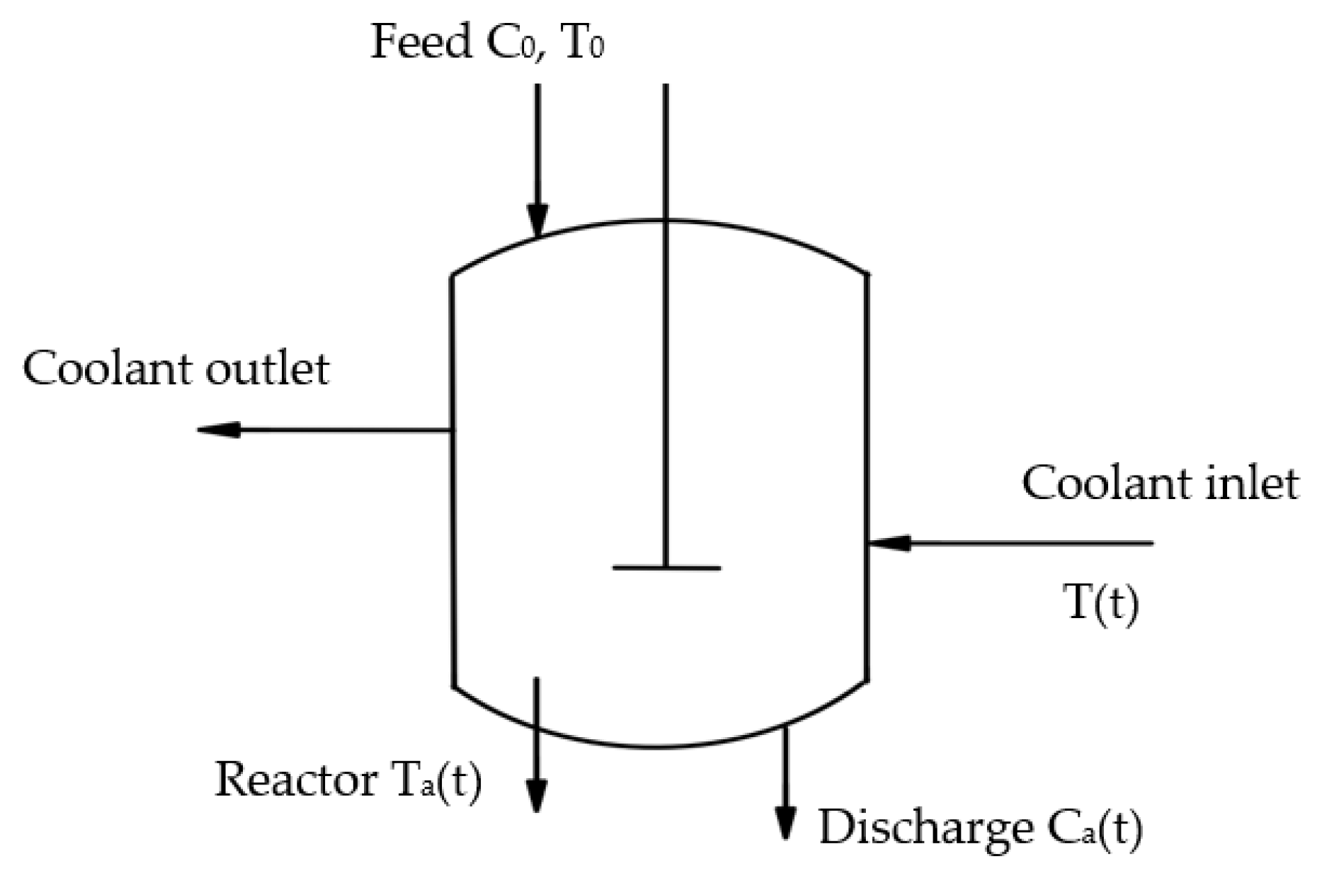
2. Model of CSTR
3. Performance Analysis of an FD Dynamic System
- (i)
- ;
- (ii)
- , ;
- (iii)
- , .
4. Fuzzy FD Filter Design
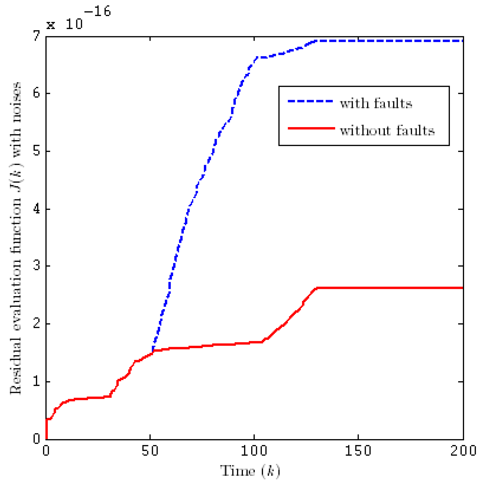
5. Numerical Example
6. Conclusions
Author Contributions
Funding
Institutional Review Board Statement
Informed Consent Statement
Data Availability Statement
Conflicts of Interest
References
- Li, Y.; Feng, Y. T-S model based L2-L∞ control for continuous stirring tank reactor. J. Jilin Univer. (Inform. Sci. Ed.) 2014, 329, 247–253. [Google Scholar]
- Chen, Z.; Cao, Y.; Ding, S.X.; Zhang, T. A Distributed canonical correlation analysis-based fault detection method for plant-wide process monitoring. IEEE Trans. Ind. Inform. 2019, 15, 2710–2720. [Google Scholar] [CrossRef]
- Gao, Z.; Cecati, C.; Ding, S.X. A survey of fault diagnosis and fault-tolerant techniques—Part I: Fault diagnosis with model-based and signal-based approaches. IEEE Trans. Ind. Electron. 2015, 62, 3757–3767. [Google Scholar] [CrossRef] [Green Version]
- Gao, Z.; Cecati, C.; Ding, S.X. A survey of fault diagnosis and fault-tolerant techniques—Part II: Fault diagnosis with knowledge-based and hybrid/active approaches. IEEE Trans. Ind. Electron. 2015, 62, 3768–3774. [Google Scholar] [CrossRef] [Green Version]
- Gao, Z.; Sheng, S. Real-time monitoring, prognosis, and resilient control for wind turbine systems. Renew. Energy 2017, 116, 1–4. [Google Scholar] [CrossRef]
- Hou, N.; Wang, Z.; Ho, D.W.; Dong, H. Robust partial-nodes-based state estimation for complex networks under deception attacks. IEEE Trans. Cybern. 2020, 50, 2793–2802. [Google Scholar] [CrossRef]
- Chen, H.; Jiang, B.; Chen, W.; Yi, H. Data-driven detection and diagnosis of incipient faults in electrical drives of high-speed trains. IEEE Trans. Ind. Electron. 2019, 66, 4716–4725. [Google Scholar] [CrossRef]
- Gao, Z.; Liu, X. An Overview on Fault Diagnosis, Prognosis and resilient control for wind turbine systems. Processes 2021, 9, 300. [Google Scholar] [CrossRef]
- Ali, N.; Hong, J. Failure detection and prevention for cyber-physical systems using ontology-based knowledge base. Computers 2018, 7, 68. [Google Scholar] [CrossRef] [Green Version]
- Dong, H.; Hou, N.; Wang, Z. Fault estimation for complex networks with randomly varying topologies and stochastic inner couplings. Automatica 2020, 112, 108734. [Google Scholar] [CrossRef]
- Zhang, Z.; Yang, G. Distributed fault detection and isolation for multiagent systems: An interval observer approach. IEEE Trans. Syst. Man Cybern. Syst. 2020, 50, 2220–2230. [Google Scholar] [CrossRef]
- Ye, D.; Chen, M.; Yang, H. Distributed adaptive event-triggered fault-tolerant consensus of multiagent systems with general linear dynamics. IEEE Trans. Cybern. 2019, 49, 757–767. [Google Scholar] [CrossRef]
- Zhu, X.; Liu, Y.; Fang, J.; Zhong, M. Fault detection for a class of linear systems with integral measurements. Sci. China Inform. Sci. 2021, 64, 1–10. [Google Scholar] [CrossRef]
- Taoufik, A.; Defoort, M.; Djemai, M.; Busawon, K.; Sánchez-Torres, J.D. Distributed global actuator fault-detection scheme for a class of linear multi-agent systems with disturbances. IFAC-PapersOnLine 2020, 53, 4202–4207. [Google Scholar] [CrossRef]
- Alikhani, H.; Meskin, N. Event-triggered robust fault diagnosis and control of linear Roesser systems: A unified framework. Automatica 2021, 128, 109575. [Google Scholar] [CrossRef]
- Zhong, M.; Ding, S.X.; Zhou, D.; He, X. An Hi/ H∞ optimization approach to event-triggered fault detection for linear discrete time systems. IEEE Trans. Autom. Control 2020, 65, 4464–4471. [Google Scholar] [CrossRef]
- Ren, W.; Gao, M.; Kang, C. Non-fragile h-infinity fault detection for nonlinear systems with stochastic communication protocol and channel fadings. Int. J. Control Autom. Syst. 2021, 19, 2150–2162. [Google Scholar] [CrossRef]
- Ma, H.; Xu, L. Cooperative fault diagnosis for uncertain nonlinear multiagent systems based on adaptive distributed fuzzy estimators. IEEE Trans. Cybern. 2020, 50, 1739–1751. [Google Scholar] [CrossRef]
- Gao, Z. Estimation and compensation for Lipschitz nonlinear discrete-time systems subjected to unknown measurement delays. IEEE. Trans. Indust. Electron. 2015, 62, 5950–5961. [Google Scholar] [CrossRef]
- Liu, X.; Gao, Z.; Zhang, A. Observer-based fault estimation and tolerant control for stochastic Takagi–Sugeno fuzzy systems with Brownian parameter perturbations. Automatica 2019, 102, 137–149. [Google Scholar] [CrossRef]
- Ji, W.; Wang, T.; Qiu, J.; Fu, S. Distributed fuzzy H∞ filtering for nonlinear multi-rate networked double-layer industrial processes. IEEE Trans. Indust. Electron. 2017, 64, 5203–5211. [Google Scholar]
- Su, X.; Shi, P.; Wu, L.; Basin, M.V. Reliable filtering with strict dissipativity for T–S fuzzy time-delay systems. IEEE Trans. Cybern. 2017, 44, 2470–2483. [Google Scholar]
- Ali, M.S.; Gunasekaran, N.; Zhu, Q. State estimation of T–S fuzzy delayed neural networks with Markovian jumping parameters using sampled-data control. Fuzzy Sets Syst. 2017, 306, 87–104. [Google Scholar]
- Chibani, A.; Chadli, M.; Ding, S.X.; Braiek, N.B. Design of robust fuzzy fault detection filter for polynomial fuzzy systems with new finite frequency specifications. Automatica 2018, 93, 42–54. [Google Scholar] [CrossRef]
- Shen, Y.; Wang, Z.; Shen, B.; Fuad, E. Alsaadi. Event-based recursive filtering for a class of nonlinear stochastic parameter systems over fading channels. Int. J. Gen. Syst. 2018, 47, 401–415. [Google Scholar] [CrossRef]
- Zhang, Z.; Su, S.; Niu, Y. Dynamic event-triggered control for interval type-2 fuzzy systems under fading channel. IEEE Trans. Cybern. 2020, 99, 1–10. [Google Scholar] [CrossRef]
- Wang, Y.; Ren, W.; Lu, Y. Fault detection for complex systems with channel fadings, randomly occurring multiple delays and infinitely distributed delays. J. Syst. Sci. Complex. 2018, 31, 419–435. [Google Scholar] [CrossRef]
- Dong, H.; Wang, Z.; Lam, J.; Gao, H. Fuzzy-model-based robust fault detection with stochastic mixed time delays and successive packet dropouts. IEEE Trans. Syst. Man Cybern. Syst. 2012, 42, 365–376. [Google Scholar] [CrossRef] [Green Version]
- Li, M.; Yu, D.; Chen, Z.; XiaHou, K.; Ji, T.; Wu, Q.H. Data-driven residual-based method for fault diagnosis and isolation in wind turbines. IEEE Trans. Sustain. Energy 2019, 10, 895–904. [Google Scholar] [CrossRef]
- Guan, X.P.; Chen, C.L. Delay-dependent guaranteed cost control for T-S fuzzy systems with time delays. IEEE Trans. Fuzzy Syst. 2004, 12, 236–249. [Google Scholar] [CrossRef]
- Wang, Z.; Ho, D.; Liu, Y.; Liu, X. Robust H∞ control for a class of nonlinear discrete time-delay stochastic systems with missing measurements. Automatica 2009, 45, 684–691. [Google Scholar] [CrossRef] [Green Version]
- Djeziri, M.; Nguyen, T.-B.-L.; Benmoussa, S.; M’Sirdi, N. Fault prognosis based on physical and stochastic models. In Proceedings of the 2016 European Control Conference, Aalborg, Denmark, 29 June–1 July 2016; pp. 2269–2274. [Google Scholar]


Publisher’s Note: MDPI stays neutral with regard to jurisdictional claims in published maps and institutional affiliations. |
© 2021 by the authors. Licensee MDPI, Basel, Switzerland. This article is an open access article distributed under the terms and conditions of the Creative Commons Attribution (CC BY) license (https://creativecommons.org/licenses/by/4.0/).
Share and Cite
Wang, Y.; Ren, W.; Liu, Z.; Li, J.; Zhang, D. T-S Fuzzy Model-Based Fault Detection for Continuous Stirring Tank Reactor. Processes 2021, 9, 2127. https://doi.org/10.3390/pr9122127
Wang Y, Ren W, Liu Z, Li J, Zhang D. T-S Fuzzy Model-Based Fault Detection for Continuous Stirring Tank Reactor. Processes. 2021; 9(12):2127. https://doi.org/10.3390/pr9122127
Chicago/Turabian StyleWang, Yanqin, Weijian Ren, Zhuoqun Liu, Jing Li, and Duo Zhang. 2021. "T-S Fuzzy Model-Based Fault Detection for Continuous Stirring Tank Reactor" Processes 9, no. 12: 2127. https://doi.org/10.3390/pr9122127