Fast and Versatile Chromatography Process Design and Operation Optimization with the Aid of Artificial Intelligence

Abstract

Preparative and process chromatography is a versatile unit operation for the capture, purification, and polishing of a broad variety of molecules, especially very similar and complex compounds such as sugars, isomers, enantiomers, diastereomers, plant extracts, and metal ions such as rare earth elements. Another steadily growing field of application is biochromatography, with a diversity of complex compounds such as peptides, proteins, mAbs, fragments, VLPs, and even mRNA vaccines. Aside from molecular diversity, separation mechanisms range from selective affinity ligands, hydrophobic interaction, ion exchange, and mixed modes. Biochromatography is utilized on a scale of a few kilograms to 100,000 tons annually at about 20 to 250 cm in column diameter. Hence, a versatile and fast tool is needed for process design as well as operation optimization and process control. Existing process modeling approaches have the obstacle of sophisticated laboratory scale experimental setups for model parameter determination and model validation. For a broader application in daily project work, the approach has to be faster and require less effort for non-chromatography experts. Through the extensive advances in the field of artificial intelligence, new methods have emerged to address this need. This paper proposes an artificial neural network-based approach which enables the identification of competitive Langmuir-isotherm parameters of arbitrary three-component mixtures on a previously specified column. This is realized by training an ANN with simulated chromatograms varying in isotherm parameters. In contrast to traditional parameter estimation techniques, the estimation time is reduced to milliseconds, and the need for expert or prior knowledge to obtain feasible estimates is reduced.

1. Introduction

One of the core concepts in high-quality separation and purification is preparative chromatography as a well-established method in biopharmaceutical manufacturing [1]. Traditionally, preparative chromatography was developed through laboratory experiments that were both time and material consuming [2,3]. However, these no longer meet today’s requirements for streamlined and personalized pharmaceutical production in ever-shorter development cycles [4,5]. Therefore, the need for faster methods for process development arises. This is further encouraged by authorities such as the American Food and Drug Administration (FDA), or the European Medicines Agency (EMA), with concepts such as Quality by Design (QbD), and Process Analytical Technology (PAT), which promote deeper process understanding in the pharmaceutical industry [6,7,8]. A promising approach to tackle this objective is the utilization of process modeling for process development. Models are based on the mathematical description of the physical and biochemical phenomena of the process. This significantly increases the level of process understanding. Other opportunities are the reduction in process development time, and enabling model-based process control strategies, and optimization. If pursued further, this leads to the complete digitalization of the plant, the so-called digital twin [9,10,11]. As a consequence, the necessity for a fast and accurate low-effort model parameter determination emerges [12,13].

The most common model for determining model parameters were purely experimental such as pulse tests for axial dispersion and bed porosity [2,14], or static and dynamic experiments for (competitive) adsorption isotherms [1,15,16]. However, these methods often suffer from high experimental effort terms of time and material consumption [2,13]. Faster methods are given by the model-based integration of correlations from typically more accessible parameters [2]. Examples are the correlations for the pore diffusion coefficient $D_{p,i}$ by Carta [17] and $k_{f,i}$ by Wilson and Geankoplis [18]. Other approaches shift the effort from the experimental to the computational side. This is accomplished by formulating the parameter estimation tasks as inverse problems. In these model-based parameter estimation techniques, the parameters are determined by fitting the model onto the real data [13,19,20]. However, expert knowledge is required to fasten this process and make it feasible, which is a drawback.

Recent approaches utilize artificial neural networks (ANN). These range from grey box modeling to the modeling of retention times in chromatography [21,22,23]. In grey box modelling, ANNs are integrated into mechanistic models to avoid the necessity of determining specific parameters by using data to describe certain phenomena [13,24]. Other chromatography research focused on predicting certain parameters from available measurements, such as isotherm parameters [12,25,26]. One of the earliest studies regarding isotherms was conducted by Gao and Engell [13], who used an ANN as the isotherm function itself to avoid a mismatch between the assumed functional form and the actual isotherm. However, the design of experiments with enough information was stated as a key issue by the authors [13]. Additionally, the development procedure has to be repeated for new systems. In a newer approach by Wang et al. [12], an ANN for mass transfer and isotherm parameter estimation was developed based on the Steric Mass Action model. The resulting ANN only needed bind–elute chromatograms with linear gradient elution for parameter estimation within milliseconds.

In this article, an artificial neural network (ANN) was utilized for isotherm parameter estimation in chromatography process modeling by analyzing the peak shapes, and their retention times, in chromatograms. This study is based on the general rate model with a competitive Langmuir isotherm to model the thermodynamic binding term. For data generation, a validated chromatography model with gradient elution was used [27]. The isotherm parameters were varied within a predefined range at three different gradients. In the training process, the ANN learned to map the resulting chromatograms to the associated parameters. This approach enabled the ANN to predict the competitive Langmuir parameters for all three-component mixtures in the specified chromatography column. However, if column parameters were inserted into the training set, this limitation could be lifted. Even for fixed column parameters, the ANN needs only to be trained once. Thus, repeated traditional parameter estimation techniques for new feed mixtures are rendered obsolete on the specified column. This leads to the benefit that the competitive Langmuir-isotherm parameters of arbitrary components can be identified with three chromatograms within milliseconds. This eliminates the need for prior knowledge of the components to obtain feasible parameter estimates and reduces the time required for the process/model development. To reduce the level of abstraction, a mixture of IgG, and two groups of Host Cell Proteins (HCPs), was used as a working example.

2. Material and Methods

2.1. Modeling

The necessary data for the ANN were generated through simulations. The simulation model depicts a three-component separation on an Ion Exchange Column (IEX) with a salt gradient. The most common chromatography models were based on a general rate model Equation (1) or a lumped pore diffusion model Equation (2) [15,27,28]. These equations describe the mass balance of the stationary phase [15]. This work utilized the lumped pore diffusion model.

$${\epsilon }_{p,i}\frac{\partial c_{p,i}}{\partial t}+\left(1-{\epsilon }_{p,i}\right)\frac{\partial q_i}{\partial t}=\frac{1}{r^2}\frac{\partial }{\partial r}\left[r^2\left({\epsilon }_{p,i}{D}_{p,i}\frac{\partial c_{p,i}}{\partial r}+\left(1-{\epsilon }_{p,i}\right)D_{S,i}\frac{\partial q_i^{\ast }}{\partial r}\right)\right]$$

(1)

$${\epsilon }_{p,i}·\frac{\partial c_{p,i}}{\partial t}+\left(1-{\epsilon }_{p,i}\right)\ast \frac{\partial q_i}{\partial t}=\frac{6}{d_P}·\frac{\left(1-{\epsilon }_S\right)}{{\epsilon }_S}·k_{eff,i}·\left(c_i-c_{p,i}\right)$$

(2)

In this, ${\epsilon }_{p,i}$ expresses the porosity of the component, $c_{p,i}$ the concentration of the component in the pores of the resin, $t$ the time, $q_i$ the loading, $d_P$ the mean diameter of the resin particle, ${\epsilon }_S$ the voidage, $k_{eff,i}$ the effective mass transport coefficient, and $c_i$ the concentration in the continuous phase [15].

The adsorption of the components on the chromatography resin can be described by various approaches [15,16,28,29,30,31,32]. In this work, the competitive Langmuir-isotherm Equation (3), which has already demonstrated its performance in (bio-) chromatography, was used [16,27,28,31,33].

$$q_i=\frac{q_{max,i}{K}_{eq,i}{c}_i}{1+{\sum }_j{K}_{eq,j}{c}_j}$$

(3)

With $q_{max,i}$ as the maximum loading capacity of component $i$ and $K_{eq,i}$ as the Langmuir-coefficient of component $i$. To include the salt dependence into Equation (3) the Langmuir-coefficient can be written as shown in Equation (4) [15].

$$q_{max,i}{K}_{eq,i}=H_i$$

(4)

The salt dependence of the maximum loading $q_{max,i}$ and the Henry-coefficient $H_i$ can then be expressed by Equations (5) and (6) and the empiric coefficients $a_{1,i}$, $a_{2,i}$, $b_{1,i}$ and $b_{2,i}$ for each component $i$ [28,34].

$$q_{max,i}=b_{1,i}{c}_{p,i}+b_{2,i}$$

(5)

$$H_i=a_{1,i}{c}_{p,i}{}^{a_{2,i}}$$

(6)

The mass transfer coefficient $k_{eff,i}$ is given by Equation (7). Here, $k_{f,i}$ is the film mass transfer coefficient, $r_p$ the particle radius, and $D_{p,i}$ the pore diffusion coefficient [35].

$$k_{eff,i}=\frac{1}{\frac{1}{k_{f,i}}+\frac{r_p}{D_{p,i}}}$$

(7)

The pore diffusion coefficient $D_{p,i}$ was calculated according to the correlation of Carta [17] and $k_{f,i}$ according to Wilson and Geankoplis [18].

The spatial discretization of the partial differential equation system was performed by a finite differences scheme. The resulting system was solved by a mixed Newton algorithm.

2.2. Dataset Generation

As previously mentioned, the dataset could be generated for an arbitrary combination of components. The working example was based on the work of Zobel-Roos et al. [27] and Kornecki et al. [36]. The working example consisted of a separation of a three-component mixture containing Immunoglobulin G (IgG), and two groups of Host Cell proteins called HCP1 and HCP2 on an IEX chromatography with three different salt gradients (3 CV, 5 CV, and 10 CV). The parameter estimation and model validation followed the model validation scheme of Sixt [37], and is described in Zobel-Roos et al. [27].

The dataset for ANN training and validation was generated by 800 simulation experiments. Based on the results of Wang et al. [38] an explicit addition of noise to each experiment was omitted. Each experiment consisted of three simulative separations at salt gradients at a steepness of 3, 5, and 10, column volumes (CV). For each experiment, the isotherm describing coefficients $a_1$, $a_2$, $b_1$ and $b_2$ of Equations (5) and (6) and the concentration of the components in the feed mixture were randomly altered after a uniform distribution. Alteration of the concentration was necessary to generate examples within and outside of the linear part of the isotherm, which was dominated by the Henry coefficient. The injection volume was constant. The variation boundaries were chosen based on an expected trade-off between the training set size, and the proof of concept in this approach. Especially high concentration variations were chosen to increase the number of nearly overloaded peaks in the training set. The variation boundaries of the IgG absorption behavior influencing values are given in

Table 1. IgG parameter boundaries for the dataset generation.

IgG	a1	a2	b1	b2	Concentration
Upper boundary	0.96 (+20%)	−2.7 (+10%)	−0.192 (+20%)	0.225 (+13%)	3 g/L (+50%)
Base Value	0.8	−3	−0.24	0.2	2 g/L
Lower Boundary	0.64 (−20%)	−3.3 (−10%)	−0.288 (−10%)	0.175 (−8.75%)	1.5 g/L (−25%)

. The effect on the isotherm is illustrated in Figure 1, which depicts the enveloping curves of all the possible isotherms within the given boundaries at two different salt concentrations.

Figure 1 shows two plots, one at low salt concentration (a) and one at high salt concentration (b), to give an impression of the isotherm behavior with rising salt concentration. The same applies to Figure 2, which depicts the enveloping curves of the two component groups HCP1 and HCP2. The corresponding data are shown in

Table 2. HCP1 parameter boundaries for the dataset generation.

HCP1	a1	a2	b1	b2	Concentration
Upper boundary	1.92 (+20%)	−2.7 (+10%)	−0.006 (+20%)	0.0113 (+13%)	0.35 g/L (+180%)
Base Value	1.6	−3	−0.0075	0.01	0.125 g/L
Lower Boundary	1.28 (−20%)	−3.3 (−10%)	−0.009 (−20%)	0.00875 (−8.75%)	0.1 g/L (−20%)

and

Table 3. HCP2 parameter boundaries for the dataset generation.

HCP2	a1	a2	b1	b2	Concentration
Upper boundary	0.36 (+20%)	−2.7 (+10%)	−0.004 (+20%)	0.0225 (+13%)	0.7 g/L (+86.6%)
Base Value	0.3	−3	−0.005	0.02	0.375 g/L
Lower Boundary	0.24 (−20%)	−3.3 (−10%)	−0.006 (−20%)	0.0175 (−8.75%)	0.35 g/L (−6.6%)

.

For faster operations on the resulting data, each concentration curve of the 1655, a long simulated chromatogram, was reduced to 400 equidistant data points with a distance of 4.14 s. For ANN input data reduction, each of the already reduced curves was additionally reduced to 39 data points by the following scheme: the first data point is the time point at which the peak reaches its maximum. The following points are the time points at predefined fractions of the maximum concentration at both sides of the peak. In this study, we chose 5% steps. An example of the data point selection scheme is illustrated in Figure 3. Because the exact points do not exist in reality or in simulations, the time points were calculated via linear interpolation between the nearest lower and higher points. This leads to a perceptible noise, which is implicitly induced by a combination of peak maximum clipping, linear interpolation, and static sample points.

This approach was chosen to reduce the effect of prior assumptions about the peak shape, such as the (exponential) Gauß-shape, on the dataset and thus on the following results. Additionally, the maximum concentration of each component in the chromatogram and the injected component masses of the feed mixture are added. Accordingly, a single dataset entry consists of 40 data points per component per gradient-steepness and the three-feed mixture masses, resulting in 363 data points per sample row in the dataset. Another approach to reducing chromatogram information into fewer points can be found in Wang et al. [12].

2.3. Artificial Neural Network

Artificial neural networks (ANN) enabled the computer-aided solution of problems that were nearly impossible or difficult to solve (within the acceptable time limits) with conventional algorithms. This includes, for example, image recognition [39]. More relevant modeling contributions were the reduction in computational effort and/or the description of not yet (sufficiently) described physico-chemical relationships [13,24,40].

Artificial Neural Networks consist of interconnected neurons, which send information in the form of activations signals over weighted connections to other neurons [39]. In order to characterize ANN, a distinction between properties, architecture, activation functions, and training can be made [39,41,42]. ANN are arranged on layers of neurons: the input layer, the last layer, the output layer, and the layers in between the so-called hidden layers [39]. Common architectures are feed forward networks, in which all the information is fed forward from the input to the output nodes, and recurrent neural networks, in which the information can be cycled back to nodes of the same or previous layers [39,41,42]. An example of the fully connected feed forward network is given in Figure 4. The activation function maps the weighted inputs of a neuron to its output. Example functions are the linear functions, or nonlinear functions, such as the sigmoid function, or the hyperbolic tangent function [39,42,43]. The process of finding the parameters of the activation function of each neuron is called training [39]. Further information on ANN can be found in Fausett [39] and Goodfellow [41].

For this study, the ANN consisted of 363 input neurons, one hidden layer with 300 neurons and a 30% dropout for generalization, and 12 output neurons. The layers were structured as a fully connected feed forward network. The activation function of all neurons was the SELU function, which showed self-normalizing properties [44]. The stochastic gradient descent, with a learning rate of 0.01, an initial moment of 0, and a batch size of 25 was used [45]. The amount of training epochs was set to 50,000, with early stopping after 20 epochs without improvement. For implementation, the Tensorflow 2 backend of Keras v. 2.4.0 with Python 3.8 was used [46,47]. All the Python programming was performed in the Spyder IDE. Calculations were performed on a Dell Precision 3630 workstation.

The input and output data for the training were rescaled to a mean of zero and standard deviation of one. After that the data were additionally scaled from −0.9 to 0.9. The dataset was randomly split into an 80% training and 20% validation data. Under these conditions, the training duration was 44 min and 17 s, without GPU support.

3. Results and Discussion

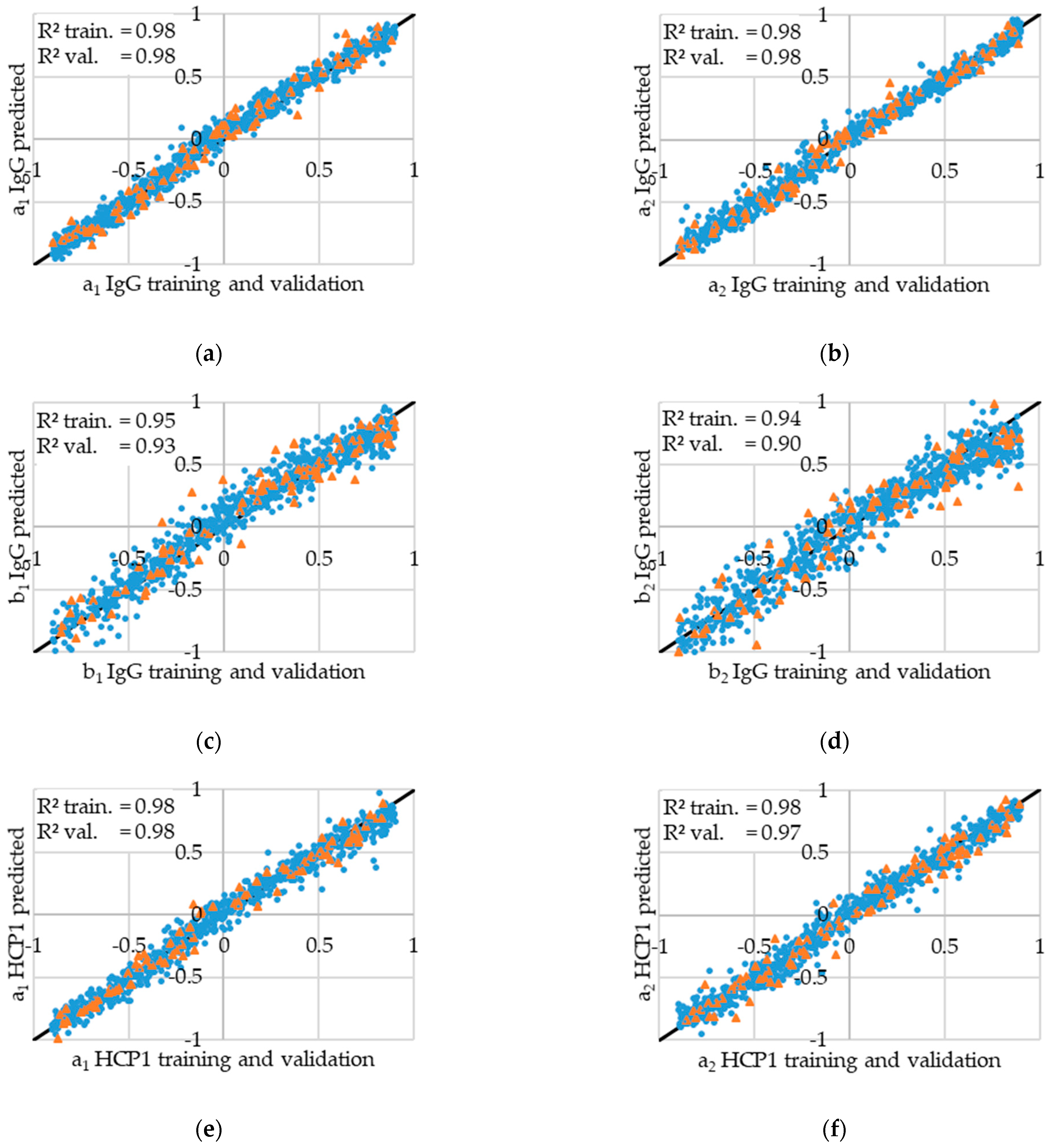
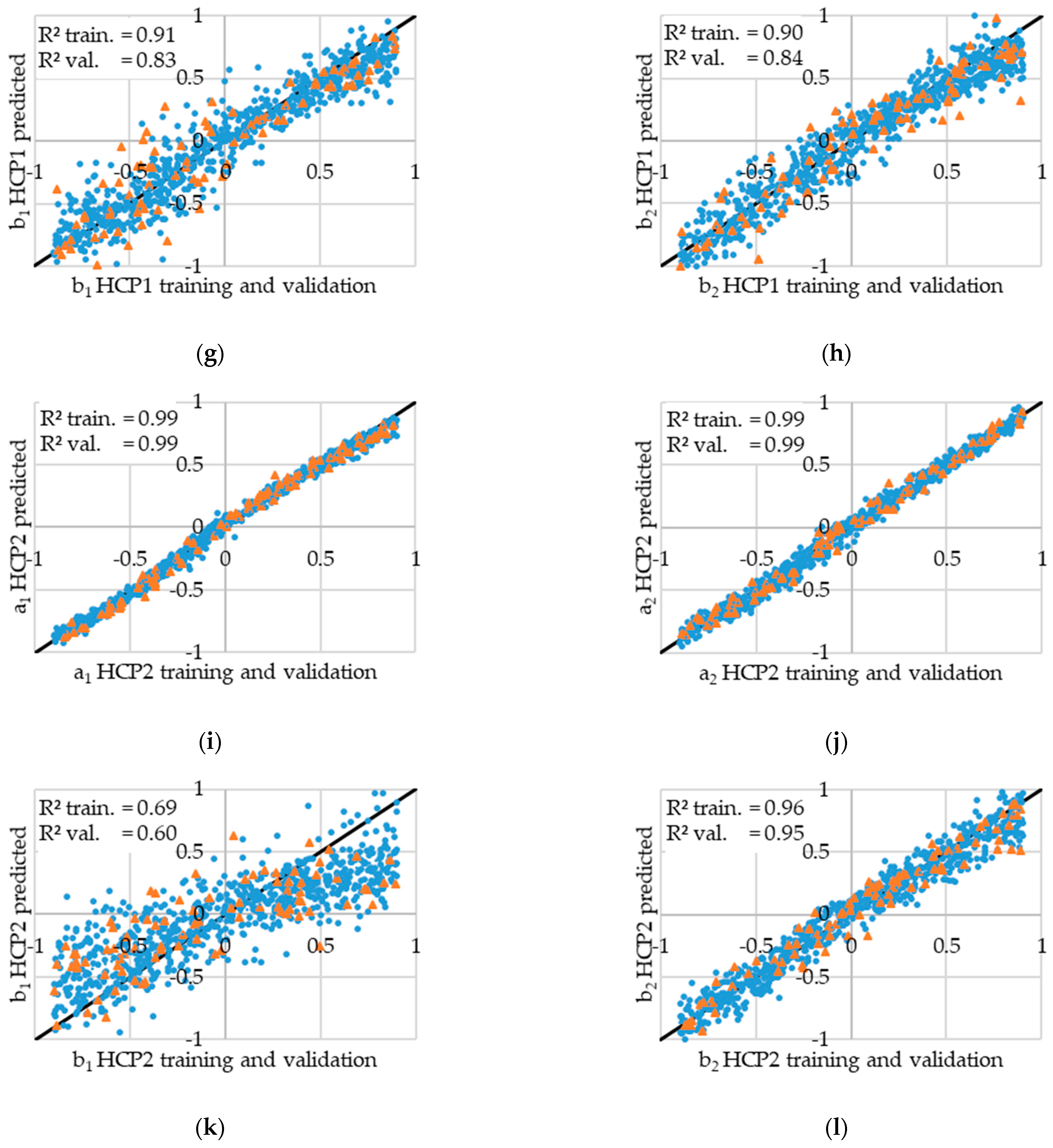
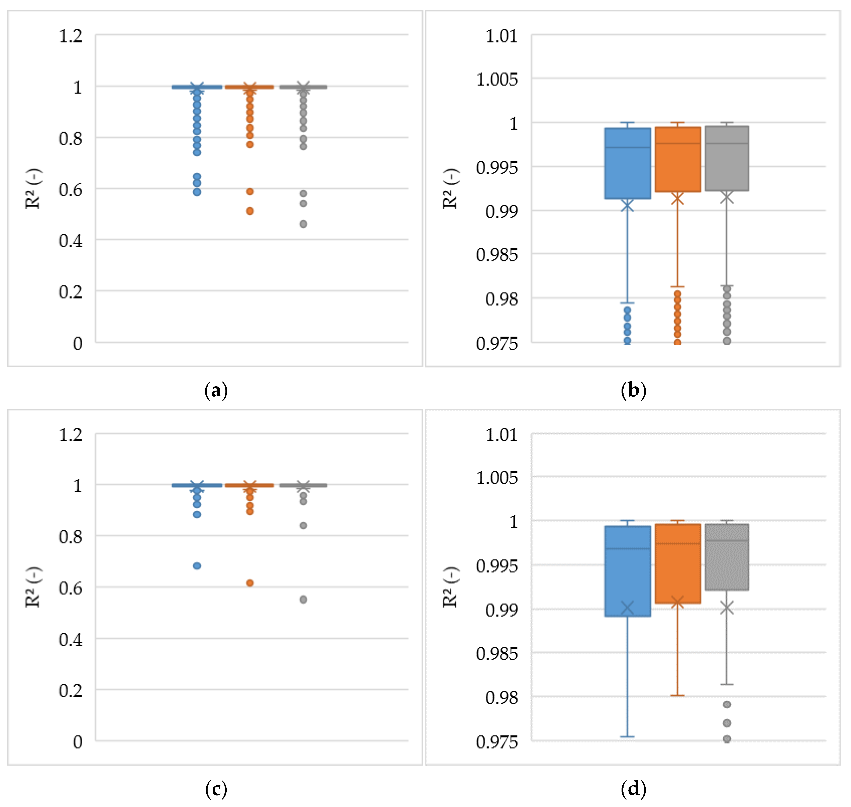
3.1. ANN Prediction Results

After the training process of the ANN was completed, the training and validation data were predicted. The prediction of a single data entry cost 200 milliseconds of computation time, including the loading of the input data and of the ANN model itself. The comparison of prediction results and original values of the coefficients from Equations (5) and (6) for all components are illustrated in Figure 5.

The best prediction performance can be seen for the parameters $a_1$ and $a_2$ for all the components, with a coefficient of determination ($R^2$) at over 0.97. The prediction performance of the maximum loading describing parameters $b_1$ and $b_2$ seems to be insufficient. This especially applies to $b_1$ of HCP2 validation set (Figure 5k) with a $R^2$ of 0.6 and to $b_1$ and $b_2$ of the HCP1 validation set with $R^2$ of 0.83 and 0.84. Similar values can be observed in the training data. This excludes overfitting as the reason for this performance. The remaining causes could be attributed to an insufficient amount of the right data, a low significance of these values on the chromatograms, or a faulty network design.

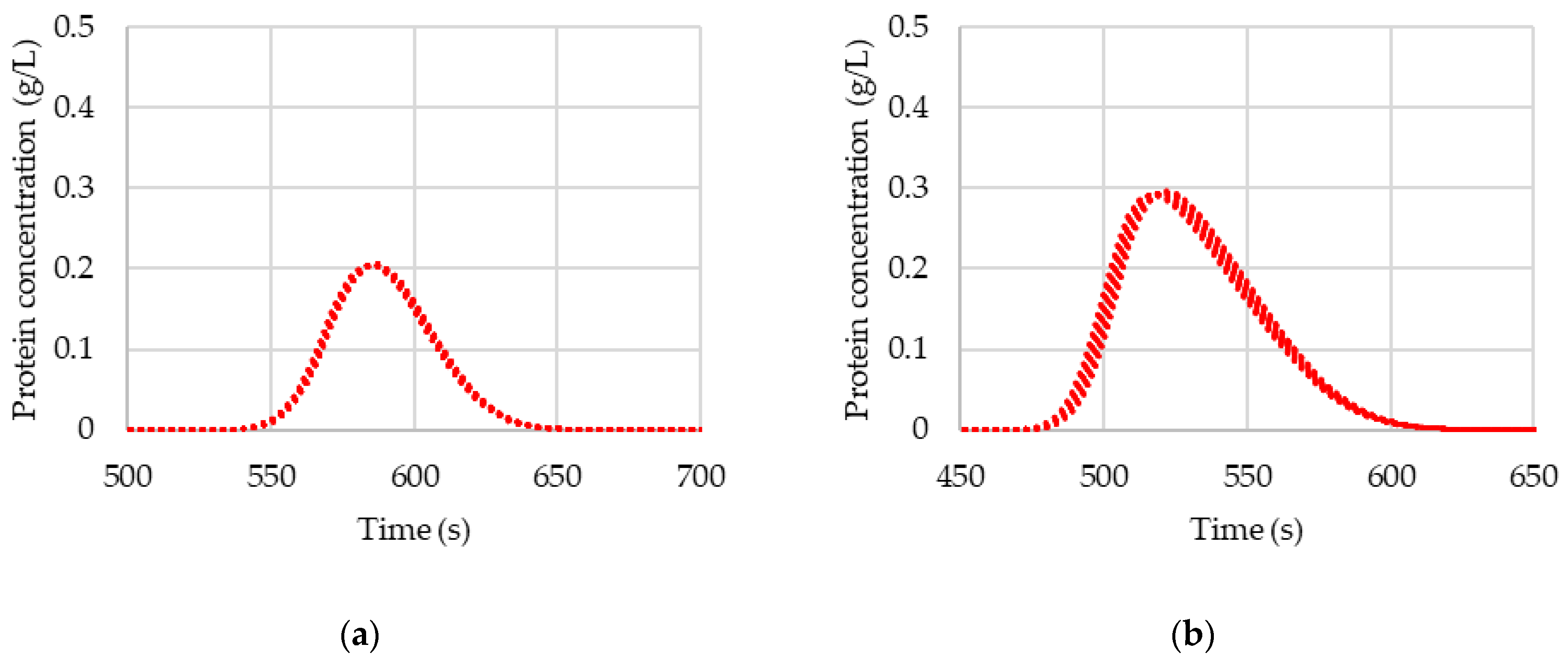
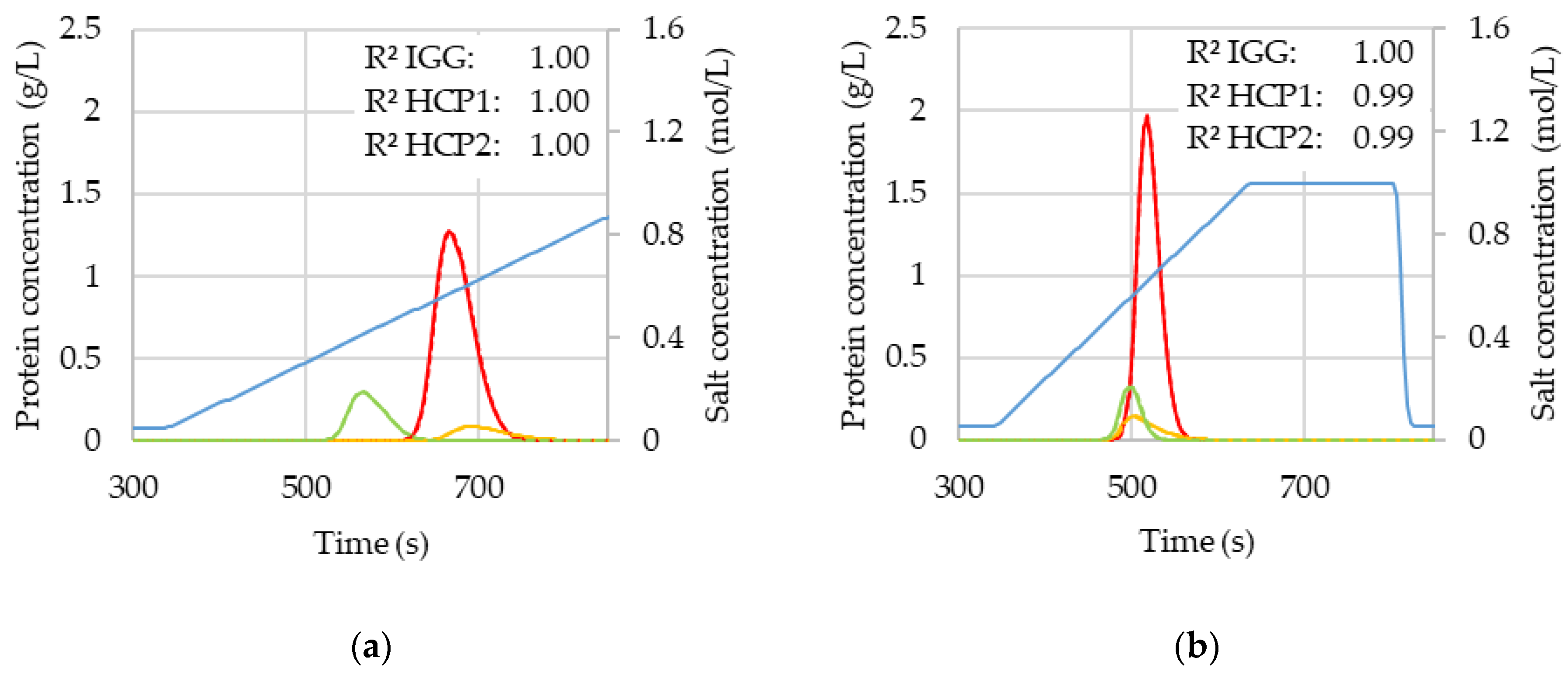
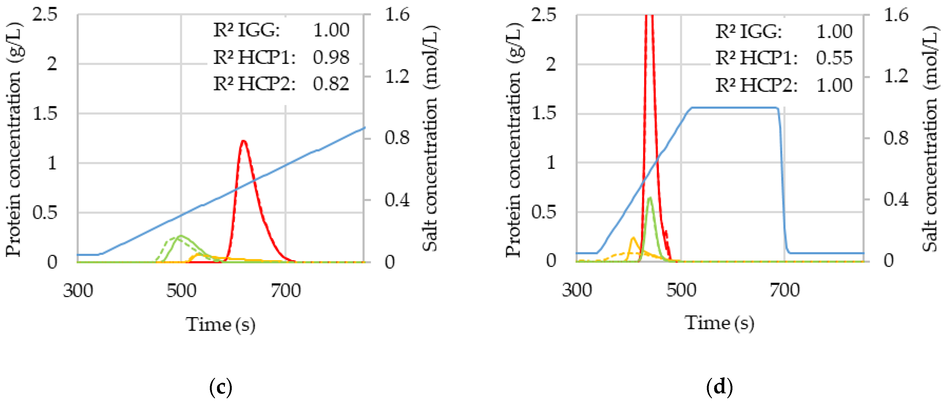
3.2. Comparison of Chromatogramms with Original and Predicted Values

To better evaluate the results, all chromatograms were re-simulated with the newly predicted values. No other parameters besides the isotherm parameters were changed. Every newly generated chromatogram was compared with its original via the $R^2$ value. In order to reduce the information of all the 2400 chromatogram comparisons into a comprehensible representation, these data are presented as box plots in Figure 6. The maximum length of the whiskers is 1.5 interquartile range (IQR). The higher zoom subplots are supplied to make the characteristic box plot values visible. The characteristic box plot values are listed in

Table 4. Values of the characteristic box plot properties from Figure 6.

Set	Q1 (25%)	Median (50%)	Q3 (75%)	Lower Whisker	Upper Whisker
Training 10 CV R2	0.991	0.997	0.999	0.979	1
Training 5 CV R2	0.992	0.998	0.999	0.981	1
Training 3 CV R2	0.992	0.998	1	0.981	1
Validation 10 CV R2	0.989	0.997	0.999	0.975	1
Validation 5 CV R2	0.99	0.997	0.999	0.980	1
Validation 3 CV R2	0.992	0.998	0.999	0.981	1

.

From Figure 6c,d and Table 4, it can be concluded that the ANN prediction model is not overfitting, and generalizes well within its previously chosen boundaries. Only a few outliers can be identified, while it should be noted that an R² lowers as the lower whisker from Table 4 already counts as such from a statistical point of view. In total, around 3% of all validation and 2.7% of all training data have an R² lower than 0.95. This leads to the conclusion that, contrary to the first impression of Figure 5, the prediction accuracy of the parameters $b_1$ and $b_2$ is already sufficient. A possible explanation for this is the fact that the significance of $b_1$ and $b_2$ rises the nearer the column loading comes to the maximum capacity. Otherwise, the separation is mostly dominated by the Henry coefficient. This claim is also supported by Figure 7, which shows a rising significance of $b_1$ at a higher concentration of HCP2.

An additional obstacle to the prediction capability may be due to the circumstance that nearly overloaded peaks and combinations of multiple overloaded peaks are underrepresented in the dataset because of the uniform distribution of the values from Table 1, Table 2 and Table 3.

A comparison between the original isotherm parameters and the predicted isotherm parameters from the validation set is shown for selected chromatograms in Figure 8. Subplots (c) and (d) are shown to give an impression of the worst performing predictions, while (a) and (b) depict nearly perfect matches of the chromatograms. It can be seen that the ANN prediction can handle shifts in peak order, non-ideal Gaussian shapes, and overlapping peaks.

3.3. Discussion

The presented approach offers, with a mean R² of [0.987, 0.993] on a 95% confidence interval of the validation set, sufficient parameter estimation capabilities, which lie within the standard error of chromatography plants. After the training step, these results are accessible within milliseconds with no change in experimental effort. Changes in the peak order and non-Gaussian peaks can be handled by the proposed approach.

The initial guess of unacceptable performance for the model parameters $b_1$ and $b_2$ concluded from Figure 5g,h,k,l, could be ignored by re-simulating the chromatograms within the estimated parameters, as illustrated in Figure 6. As mentioned earlier, the low significance of the parameters $b_1$ and $b_2$ in the investigated variable boundaries at low concentrations, and the underlying uniform distribution of these variables, should prove to be the root causes of this phenomenon. Additionally, breakthroughs were systematically excluded, so that only limited data at maximum loading capacity are available. The reasoning for these exclusions is in the simplification of the input data for the ANN. The performance of the presented approach could therefore be improved by increasing the data at the upper boundary of the column load without over-weighting them in the dataset. Moreover, the dataset boundaries should consider the field of application. For example, as an initial model parameter estimator for unknown components, the dataset should cover a wider range of parameter variation, while for the real-time parameter estimation tool around a predefined point of operation, a much smaller range should be necessary to either increase precision or reduce the amount of training data. In general, a trade-off between the dataset size, accuracy, and covered parameter range has to be made.

The drawbacks of this specific ANN are its limitation to exactly three components on the IEX within the learned variable bounds owing to the assumption of a competitive isotherm. However, the competitive isotherm in the physico-chemical model more realistically describes adsorption and desorption for a component mixture [1,15,16].

4. Conclusions

In this study, an artificial neural network (ANN) for predicting isotherm parameters in gradient elution chromatography modeling has been presented. The ANN’s capabilities are shown for a three-component protein mixture on IEX chromatography. After the training of the ANN model, three chromatograms with 3 CV, 5 CV, and 10 CV linear gradients were used to estimate 12 isotherm parameters, at four per component, within milliseconds. This was achieved with an excellent precision of the coefficient of determination greater than 0.95 for 97% of the examined chromatograms. Through the chosen peak description approach, a priori assumptions about the peak shape are rendered obsolete, and allow a wide application range. The generalization capability of the ANN was shown on a separate validation set with sufficient accuracy by re-simulating the chromatograms within the estimated isotherm parameters.

After the ANN is trained, the model can be used to estimate the isotherm parameters of unknown components as long as they lie within its training boundaries. This offers the possibility of drastically reducing the experimental and computational effort and enables non-experts to perform model parameter estimations with sufficient accuracy. Furthermore, this method offers the opportunity for real-time parameter estimates for the chromatographic process control due to its rapid calculation times and exceptional accuracy. Further studies will investigate the extension of the ANN’s abilities to estimate additional model parameters and isotherms towards a model-based autonomous process operation in combination with the PAT-methods [5,35,48].

References

1. Guiochon, G. Preparative liquid chromatography. J. Chromatogr. A 2002, 965, 129–161. [Google Scholar] [CrossRef]
2. Altenhöner, U.; Meurer, M.; Strube, J.; Schmidt-Traub, H. Parameter estimation for the simulation of liquid chromatography. J. Chromatogr. A 1997, 769, 59–69. [Google Scholar] [CrossRef]
3. Eisele, P.; Killpack, R. Propene. Ullmann’s Encyclopedia of Industrial Chemistry; Wiley: Chichester, UK, 2010; p. 101. ISBN 3527306730. [Google Scholar]
4. Zobel-Roos, S.; Schmidt, A.; Mestmäcker, F.; Mouellef, M.; Huter, M.; Uhlenbrock, L.; Kornecki, M.; Lohmann, L.; Ditz, R.; Strube, J. Accelerating Biologics Manufacturing by Modeling or: Is Approval under the QbD and PAT Approaches Demanded by Authorities Acceptable Without a Digital-Twin? Processes 2019, 7, 94. [Google Scholar] [CrossRef] [Green Version]
5. Helgers, H.; Schmidt, A.; Lohmann, L.J.; Vetter, F.L.; Juckers, A.; Jensch, C.; Mouellef, M.; Zobel-Roos, S.; Strube, J. Towards Autonomous Operation by Advanced Process Control—Process Analytical Technology for Continuous Biologics Antibody Manufacturing. Processes 2021, 9, 172. [Google Scholar] [CrossRef]
6. European Medicines Agency. EU Guidelines for Good Manufacturing Practice for Medicinal Products for Human and Veterinary Use—Annex 15: Qualification and Validation. Available online: https://www.ema.europa.eu/en/human-regulatory/research-development/scientific-guidelines/quality/quality-quality-design-qbd (accessed on 5 October 2021).
7. International Council for Harmonisation of Technical Requirements for Pharmaceuticals for Human Use. ICH-Endorsed Guide for ICH Q8/Q9/Q10 Implementation, 6 December. Available online: https://database.ich.org/sites/default/files/Q8_Q9_Q10_Q%26As_R4_Points_to_Consider_0.pdf (accessed on 22 October 2021).
8. Guidance for Industry PAT—A Framework for Innovative Pharmaceutical Development; Manufacturing, and Quality Assurance, U.S. Department of Health and Human Services: Washington, DC, USA, 2004.
9. Jones, D.; Snider, C.; Nassehi, A.; Yon, J.; Hicks, B. Characterising the Digital Twin: A systematic literature review. CIRP J. Manuf. Sci. Technol. 2020, 29, 36–52. [Google Scholar] [CrossRef]
10. Schmidt, A.; Helgers, H.; Vetter, F.; Juckers, A.; Strube, J. Digital Twin of mRNA-Based SARS-COVID-19 Vaccine Manufacturing towards Autonomous Operation for Improvements in Speed, Scale, Robustness, Flexibility and Real-Time Release Testing. Processes 2021, 9, 748. [Google Scholar] [CrossRef]
11. Gerogiorgis, D.I.; Castro-Rodriguez, D. A Digital Twin for Process Optimisation in Pharmaceutical Manufacturing. In Proceedings of the 31st European Symposium on Computer Aided Process Engineering, Istanbul, Turkey, 6–9 June 2021; pp. 253–258. [Google Scholar] [CrossRef]
12. Wang, G.; Briskot, T.; Hahn, T.; Baumann, P.; Hubbuch, J. Estimation of adsorption isotherm and mass transfer parameters in protein chromatography using artificial neural networks. J. Chromatogr. A 2017, 1487, 211–217. [Google Scholar] [CrossRef]
13. Gao, W.; Engell, S. Neural Network-Based Identification of Nonlinear Adsorption Isotherms. IFAC Proc. Vol. 2004, 37, 721–726. [Google Scholar] [CrossRef]
14. Hejtmánek, V.; Schneider, P. Axial dispersion under liquid-chromatography conditions. Chem. Eng. Sci. 1993, 48, 1163–1168. [Google Scholar] [CrossRef]
15. Guiochon, G. Fundamentals of Preparative and Nonlinear Chromatography, 2nd ed.; Elsevier: Amsterdam, The Netherland, 2006; ISBN 978-0123705372. [Google Scholar]
16. Seidel-Morgenstern, A.; Guiochon, G. Modelling of the competitive isotherms and the chromatographic separation of two enantiomers. Chem. Eng. Sci. 1993, 48, 2787–2797. [Google Scholar] [CrossRef]
17. Carta, G.; Rodrigues, A.E. Diffusion and convection in chromatographic processes using permeable supports with a bidisperse pore structure. Chem. Eng. Sci. 1993, 48, 3927–3935. [Google Scholar] [CrossRef]
18. Wilson, E.J.; Geankoplis, C.J. Liquid Mass Transfer at Very Low Reynolds Numbers in Packed Beds. Ind. Eng. Chem. Fundam. 1966, 5, 9–14. [Google Scholar] [CrossRef]
19. Dose, E.V.; Jacobson, S.; Guiochon, G. Determination of isotherms from chromatographic peak shapes. Anal. Chem. 1991, 63, 833–839. [Google Scholar] [CrossRef]
20. von Lieres, E.; Schnittert, S.; Püttmann, A.; Leweke, S. Chromatography Analysis and Design Toolkit (CADET). Chem. Ing. Tech. 2014, 86, 1626. [Google Scholar] [CrossRef]
21. Golubović, J.; Protić, A.; Zečević, M.; Otašević, B.; Mikić, M. Artificial neural networks modeling in ultra performance liquid chromatography method optimization of mycophenolate mofetil and its degradation products. J. Chemom. 2014, 28, 567–574. [Google Scholar] [CrossRef]
22. Malenović, A.; Jančić-Stojanović, B.; Kostić, N.; Ivanović, D.; Medenica, M. Optimization of Artificial Neural Networks for Modeling of Atorvastatin and Its Impurities Retention in Micellar Liquid Chromatography. Chromatographia 2011, 73, 993–998. [Google Scholar] [CrossRef]
23. E Madden, J.; Avdalovic, N.; Haddad, P.; Havel, J. Prediction of retention times for anions in linear gradient elution ion chromatography with hydroxide eluents using artificial neural networks. J. Chromatogr. A 2001, 910, 173–179. [Google Scholar] [CrossRef]
24. Asprion, N.; Böttcher, R.; Pack, R.; Stavrou, M.-E.; Höller, J.; Schwientek, J.; Bortz, M. Gray-Box Modeling for the Optimization of Chemical Processes. Chem. Ing. Tech. 2018, 91, 305–313. [Google Scholar] [CrossRef]
25. Anderson, R.; Biong, A.; Gómez-Gualdrón, D.A. Adsorption Isotherm Predictions for Multiple Molecules in MOFs Using the Same Deep Learning Model. J. Chem. Theory Comput. 2020, 16, 1271–1283. [Google Scholar] [CrossRef]
26. Mahmoodi, F.; Darvishi, P.; Vaferi, B. Prediction of coefficients of the Langmuir adsorption isotherm using various artificial intelligence (AI) techniques. J. Iran. Chem. Soc. 2018, 15, 2747–2757. [Google Scholar] [CrossRef]
27. Zobel-Roos, S.; Mouellef, M.; Ditz, R.; Strube, J. Distinct and Quantitative Validation Method for Predictive Process Modelling in Preparative Chromatography of Synthetic and Bio-Based Feed Mixtures Following a Quality-by-Design (QbD) Approach. Processes 2019, 7, 580. [Google Scholar] [CrossRef] [Green Version]
28. Zobel-Roos, S. Entwicklung, Modellierung und Validierung von Integrierten Kontinuierlichen Gegenstrom-Chromatographie-Prozessen. Ph.D. Thesis, Technische Universität Clausthal, Clausthal-Zellerfeld, Germany, 2018. [Google Scholar]
29. Mollerup, J. A Review of the Thermodynamics of Protein Association to Ligands, Protein Adsorption, and Adsorption Isotherms. Chem. Eng. Technol. 2008, 31, 864–874. [Google Scholar] [CrossRef]
30. Brooks, C.A.; Cramer, S.M. Steric mass-action ion exchange: Displacement profiles and induced salt gradients. AIChE J. 1992, 38, 1969–1978. [Google Scholar] [CrossRef]
31. Carta, G.; Jungbauer, A. Protein Chromatography; Wiley: Chichester, UK, 2010; ISBN 9783527318193. [Google Scholar]
32. Langmuir, I. The adsorption of gases on plane surfaces of glass, mica and platinum. J. Am. Chem. Soc. 1918, 40, 1361–1403. [Google Scholar] [CrossRef] [Green Version]
33. Leśko, M.; Åsberg, D.; Enmark, M.; Samuelsson, J.; Fornstedt, T.; Kaczmarski, K. Choice of Model for Estimation of Adsorption Isotherm Parameters in Gradient Elution Preparative Liquid Chromatography. Chromatographia 2015, 78, 1293–1297. [Google Scholar] [CrossRef] [PubMed] [Green Version]
34. Seidel-Morgenstern, A. Experimental determination of single solute and competitive adsorption isotherms. J. Chromatogr. A 2004, 1037, 255–272. [Google Scholar] [CrossRef]
35. Vetter, F.; Zobel-Roos, S.; Strube, J. PAT for Continuous Chromatography Integrated into Continuous Manufacturing of Biologics towards Autonomous Operation. Processes 2021, 9, 472. [Google Scholar] [CrossRef]
36. Kornecki, M.; Schmidt, A.; Lohmann, L.; Huter, M.; Mestmäcker, F.; Klepzig, L.; Mouellef, M.; Zobel-Roos, S.; Strube, J. Accelerating Biomanufacturing by Modeling of Continuous Bioprocessing—Piloting Case Study of Monoclonal Antibody Manufacturing. Processes 2019, 7, 495. [Google Scholar] [CrossRef] [Green Version]
37. Sixt, M.; Uhlenbrock, L.; Strube, J. Toward a Distinct and Quantitative Validation Method for Predictive Process Modelling—On the Example of Solid-Liquid Extraction Processes of Complex Plant Extracts. Processes 2018, 6, 66. [Google Scholar] [CrossRef] [Green Version]
38. Wang, C.; Engell, S.; Hanisch, F. Neural network-based identification and mpc control of smb chromatography. IFAC Proc. Vol. 2002, 35, 31–36. [Google Scholar] [CrossRef] [Green Version]
39. Fausett, L.V. Fundamentals of Neural Networks: Architectures, Algorithms, and Applications; Prentice Hall: Englewood Cliffs, NJ, USA, 1994; ISBN 0-13-334186-0. [Google Scholar]
40. Hagge, T.; Stinis, P.; Yeung, E.; Tartakovsky, A.M. Solving Differential Equations with Unknown Constitutive Relations as Recurrent Neural Networks. 2017. Available online: https://arxiv.org/pdf/1710.02242 (accessed on 22 October 2021).
41. Goodfellow, I.; Bengio, Y.; Courville, A. Deep Learning; The MIT Press: Cambridge, MA, USA, 2016; ISBN 978-0-262-03561-3. [Google Scholar]
42. Kruse, R.; Borgelt, C.; Braune, C.; Klawonn, F.; Moewes, C.; Steinbrecher, M. Computational Intelligence; Springer Fachmedien Wiesbaden: Wiesbaden, Germany, 2015; ISBN 978-3-658-10903-5. [Google Scholar]
43. Stanley, K.O.; Miikkulainen, R. Evolving Neural Networks through Augmenting Topologies. Evol. Comput. 2002, 10, 99–127. [Google Scholar] [CrossRef] [PubMed]
44. Klambauer, G.; Unterthiner, T.; Mayr, A.; Hochreiter, S. Self-Normalizing Neural Networks. In Proceedings of the 31st International Conference on Neural Information Processing Systems, Long Beach, CA, USA, 4–9 December 2017. [Google Scholar]
45. Sutskever, I.; Martens, J.; Dahl, G.; Hinton, G. On the importance of initialization and momentum in deep learning. In Proceedings of the 30th International Conference on Machine Learning, Atlanta, GA, USA, 16–21 June 2013; Dasgupta, S., McAllester, D., Eds.; PMLR: Atlanta, GA, USA, 2013; pp. 1139–1147. [Google Scholar]
46. Abadi, M.; Agarwal, A.; Barham, P.; Brevdo, E.; Chen, Z.; Citro, C.; Corrado, G.S.; Davis, A.; Dean, J.; Devin, M.; et al. Tensorflow: Large-Scale Machine Learning on Heterogeneous Distributed Systems. 2015. Available online: https://static.googleusercontent.com/media/research.google.com/en//pubs/archive/45166.pdf (accessed on 22 October 2021).
47. Chollet, F. Keras. 2015. Available online: https://keras.io (accessed on 22 October 2021).
48. Zobel-Roos, S.; Mouellef, M.; Siemers, C.; Strube, J. Process Analytical Approach towards Quality Controlled Process Automation for the Downstream of Protein Mixtures by Inline Concentration Measurements Based on Ultraviolet/Visible Light (UV/VIS) Spectral Analysis. Antibodies 2017, 6, 24. [Google Scholar] [CrossRef] [PubMed] [Green Version]
Figure 1. Enveloping isotherm curves of IgG with the parameters from Table 1: (a) at 0.05 mol/L salt concentration and (b) 0.6 mol/L salt concentration.
Processes 09 02121 g001
Figure 2. Enveloping isotherm curves of HCP1 (yellow curves) and HCP2 (green curves) with the parameters from Table 2 and Table 3: (a) at 0.05 mol/L salt concentration and (b) 0.6 mol/L salt concentration.
Processes 09 02121 g002
Figure 3. Scheme of the data point selection. The blue curve is the original concentration curve. The orange dots are the points, at which the time is taken as data point for the dataset. The first point starts at the maximum. The following points are left and right of the maximum at 95%, 90%, descending in 5% steps until 5% of the maximum concentration is reached.
Processes 09 02121 g003
Figure 4. An example of a fully connected feed forward network with two input neurons, two neurons in the hidden layer, and one output neuron.
Processes 09 02121 g004
Figure 5. Predicted parameter values over training and validation data of all components. Training data are shown as blue dots. Validation data are shown as orange triangles. The black line represents the bisecting line. Every point, which lies directly on the bisecting line, is a perfect prediction. The coefficient of determination (R2) of training (R2 train.), and validation (R2 val.) set, are shown in the upper left corner of each panel. The prediction results of a 1 , a 2 , b 1 , and b 2 are shown in order for IgG in (ad), for HCP1 in (eh) and for HCP2 in (il).
Processes 09 02121 g005aProcesses 09 02121 g005b
Figure 6. Box plots of the R2 of chromatograms with the predicted parameters over the chromatograms with the original parameters. Blue box plots represent 10 CV salt gradient, orange represent 5 CV salt gradient chromatograms, and 3 CV salt gradient chromatograms are represented as grey box plots: (a) shows the training set data at full scale. (b) Shows the training set data R2 in a high zoom state; (c) shows the validation data R2 in full range, while (d) shows the validation data R2 in high zoom.
Processes 09 02121 g006
Figure 7. Sensitivity analysis of the parameter b 1 of HCP2 at HCP2 concentrations of (a) 0.375 g/L and (b) 0.7 g/L (upper limit) at a 10 CV salt gradient. Each plot consists of 40 chromatograms with b 1 ranging from the lower to the upper limit in equidistant steps. The maximum retention time difference is 0 s in (a) and 5 s in (b).
Processes 09 02121 g007
Figure 8. Comparison of four chromatograms with original and ANN predicted isotherm parameters from the validation set. In all subplots, the protein group HCP1 is yellow, the protein group HCP2 is green, and the IgG is red. Solid lines represent the chromatograms original isotherm parameters. Dashed lines represent the chromatograms with ANN predicted isotherm parameters: (a) depicts a chromatogram comparison at 10 CV, (b) is another comparison at 5 CV, (c) depicts one of the outliers at 10 CV, and (d) is the worst outlier at 3 CV.
Processes 09 02121 g008aProcesses 09 02121 g008b