The Role of Stochastic Time-Variations in Turbulent Stresses When Predicting Drop Breakup—A Review of Modelling Approaches

Abstract

Many industrially relevant emulsification devices are of the high-energy type, where drop deformation and subsequent breakup, take place due to intense turbulent fluid–drop interactions. This includes high-pressure homogenizers as well as rotor-stator mixers (also known as high-shear mixers) of various designs. The stress acting on a drop in a turbulent flow field varies over time, occasionally reaching values far exceeding its time-averaged value, but only during limited stretches of time, after which it decreases down to low values again. This it is one factor separating turbulent from laminar emulsification. This contribution reviews attempts to take this intermittently time-varying stress into account in models predicting the characteristic drop diameter resulting from emulsification experiments, focusing on industrially applicable emulsification devices. Two main frameworks are discussed: the Kolmogorov–Hinze framework and the oscillatory resonance framework. Modelling suggestions are critically discussed and compared, with the intention to answer how critical it is to correctly capture this time-varying stress in emulsification modelling. The review is concluded by a list of suggestions for future investigations.

1. Introduction

Emulsion formation under turbulent flow conditions has a large industrial relevance, with applications ranging from food, pharmaceutical and petrochemical to general chemical processing. The so-called high-energy methods (e.g., high-pressure homogenizers, HPHs and rotor-stator mixers, RSMs) remain the most common choice in an industrial setting, due to their scalability and their possibilities for running in continuous mode of operation. The low-energy method (e.g., phase inversion and cross-flow membrane emulsification) remains interesting due to its substantially higher thermodynamic efficiency, but is still not used as extensively.

Emulsification of low to intermediary (emulsion) viscosities (e.g., breakup of fat globules in dairy processing) is typically carried out using HPHs whereas high-viscosity systems (e.g., mayonnaise production) are typically processed using RSMs. A cut-off between methods at 200 mPa s has been suggested [1].

In both devices, drop breakup takes place in a decaying turbulent jet, either created downstream of the narrow gap of the valve-homogenizer, or downstream of the stator screen in the RSM [2]. Consequently, there is a large interest in predicting the critical drop size resulting from turbulent emulsification in processing equipment. Such an interest comes partially from an industrial perspective, where reliable predictive tools would allow for fast optimization of operating conditions, process lines and device geometries. However, there is also a more fundamental scientific interest in understanding how the details of turbulent flows interact with interfacial dynamics to give rise to deformation and breakup [3,4,5,6]. Although, turbulent drop breakup phenomena have been studied and discussed at least since the 1940s and 1950s [7,8], there is not yet a commonly accepted procedure for making valid and reliable predictions under industrially relevant conditions [2].

Three main frameworks for predicting drop breakup under turbulent emulsification can be seen in the literature: (i) the extended Kolmogorov–Hinze framework for estimating the largest drop surviving prolonged exposure to a turbulent field [7,8,9,10,11], (ii) the population balance equation (PBE) framework for predicting the dynamic evolution of the drop size-distribution [12,13,14,15,16] and (iii) the oscillatory resonance mechanism framework for predicting critical drop diameters [5,17,18].

Whereas originally proposed as a scaling law, the Kolmogorov–Hinze framework (i) is essentially a stress balance where the largest drop surviving prolonged exposure is predicted by equating disruptive and restoring stress [7,8,9,19]. The PBE framework (ii) is a set of conservation laws describing the transport of drop volume between size classes, closed by specifying a breakup frequency function (together with its fragment size distribution and, if present, by a coalescence frequency function) [12]. The oscillatory resonance mechanism framework (iii) suggests that drop breakup occurs once a drop has been critically deformed and, therefore, utilizes the dynamic deformation resulting from the sequence of eddy interactions to predict breakup probability [5].

Predicting turbulent breakup constitutes a considerable challenge for several reasons. One challenge is that there is no general consensus on which primary turbulent property causes breakup from a mechanistic perspective. This is especially clear when comparing different theoretical suggestions for the breakup frequency needed in the PBE framework. Solsvik et al. [15] identified six principally different classes of such breakup frequency models based on what the respective authors assume to be the fundamental mechanism of breakup (see [16] for a similar discussion resulting in five classes).

Another challenge (the one that will be the focus of this review) is that these turbulent quantities responsible for deforming and breaking drops in turbulent flows (as opposed to those acting on a drop in a laminar flow field), are stochastic. The dissipation rate of turbulent kinetic energy (TKE) is an illustrative example, since it plays a critical role in most applications of the three frameworks. As an illustration, Figure 1 shows the instantaneous dissipation rate of TKE as a function of time in a homogenous and isotropic turbulent flow at a high Reynolds number, as obtained from a numerical experiment using dynamic numerical simulation (DNS) in a developed turbulent channel flow [20,21,22]. The vertical axis has been normalized with the time-averaged value (calculated across a substantially longer time interval than what is displayed in the figure). As seen in the figure, the dissipation rate of TKE varies with time—it displays short periods of instantaneous values far exceeding its time-averaged value, followed by stretches of lower values. Note that a drop placed in such a turbulent field will experience this instantaneous, highly fluctuating value rather than the time-averaged value.

These stochastic time-variations in turbulent quantities can be attributed to a broader class of phenomena referred to as ‘intermittency’ in the turbulence literature. Comprehensive reviews of intermittency phenomena can be found elsewhere [23,24,25,26,27,28,29]. From an etymological perspective, the term ‘intermittency’ refers to the fact that turbulent signals are ‘intermittent’ in the sense that they behave as in Figure 1: intermittingly going through streaks of high and low values. Another consequence of intermittency is that the probability density function of these properties shows a pronounced tailing behavior where exceedingly high values are occasionally obtained, but with a low probability. The full complexity of intermittent behavior in turbulence is beyond the scope of this contribution. In addition, it could be hypothesized that several aspects of intermittency could come into play when attempting to obtain a full understanding of turbulent emulsification. This review will, however, focus on the specific consequence of the time-varying turbulent stress arising in such a flow (as seen in Figure 1).

That this stochastic time-varying behavior of turbulent stresses plays a role in turbulent drop breakup was realized already by Kolmogorov [7] in his seminal paper from 1949. Consequently, this phenomenon has been included (although not always explicitly) in a large number of breakup models, in all three of the abovementioned frameworks. There is, however, no general consensus on which of the many suggestions for taking stochastic time-variations in turbulent stresses into account is the most suitable in a predictive modelling setting of turbulent emulsifications. Nor is there any consensus under which conditions the phenomenon needs to be included to capture the physics of the problem. In fact, the most commonly found version of the Kolmogorov–Hinze framework used in contemporary studies, typically neglects it altogether, and assumes that the drop experiences a continuous stress given by the time-averaged level [9,30,31] (see discussion in Section 4).

The intention with this contribution is to critically review the different attempts to include stochastic time-variations in modelling turbulent breakup, focusing on the two modelling frameworks intended to predict the largest drop size surviving a turbulent device, e.g., the Kolmogorov–Hinze framework and the oscillatory resonance framework. (A comprehensive discussion of the role of intermittency modelling in the PBE framework can be found elsewhere [15].) Of special relevance to this review is the question under which conditions the modelling choice we make in including stochastic time-variations in stresses play a role in predicting the effect of emulsification in practically relevant devices.

The review is organized as follows: Section 2 gives a brief overview of the contrasting case when a viscous drop deforms in a steady laminar velocity gradient—in order to highlight how the stochastic time-variations of stresses set turbulent drop breakup apart. Section 3 gives an introduction to the turbulent phenomena giving rise to the stochastic time-variations. Section 4 looks at the Kolmogorov–Hinze framework, first reviewing its traditional form and then turning to the different extensions that have been suggested to include this effect. Section 5 reviews the oscillatory resonance framework and Section 6 concludes the review by comparing approaches, identifying the need for future investigations and summarizing the current state-of-the-art of the field.

2. Laminar Viscous Breakup—A Contrasting Case

Much of the turbulent drop breakup literature has been developed as extensions and re-evaluations of laminar breakup theory. This is especially true when considering the Kolmogorov–Hinze theory and the turbulent breakup of a drop that is large in comparison to the turbulent structures breaking it [32]. An interesting difference between laminar and turbulent breakup is the fact that the stress acting on a drop under laminar conditions is constant (or varies deterministically) whereas the instantaneous stress acting on a drop in a turbulent flow behaves as in Figure 1 showing a stochastic time-variation. Therefore, a brief look at laminar breakup will prove valuable as a contrasting case when continuing to how these time-variations are modelled in turbulent breakup.

Consider a drop dispersed in a large quantity of a continuous phase fluid (e.g., a drop of oil in a basin of water). This pre-emulsion is placed in a four-roller mill (see Figure 2A) where the gentle rotation of the cylinders gives rise to a constant laminar shear flow with a velocity field given by Figure 2B (provided that the rotor speed is sufficiently low). Taylor [33] first observed that drops placed in such a flow deform by elongation in the direction perpendicular to the velocity gradients. Once critically deformed, the drop breaks. How much each drop needs to be deformed before it breaks is a function of the viscosity ratio between disperse and continuous phase; more viscous drops can endure higher degrees of deformation [34].

Mechanistically, we can understand this deformation (and, hence, the resulting breakup) from looking at a stress balance [33,35], where the disruptive stress is given by the continuous phase dynamic viscosity, μ_C, multiplied by the magnitude of the velocity gradient, G:

$${\sigma }_{LV}~2\cdot {\mu }_C\cdot \left|G\right|.$$

(1)

This is counter-acted by a restoring stress created by the Laplace pressure (given by the pressure difference between the tip of the deformed drop and its center):

$${\sigma }_{stab}~\frac{\gamma }{D},$$

(2)

where γ is the interfacial tension and D is the (un-deformed) drop diameter. The ratio of disrupting to stabilizing stresses defines a laminar capillary number,

$$C{a}_{LV}=\frac{2\cdot {\mu }_C\cdot \left|G\right|\cdot D}{\gamma }.$$

(3)

For the example of the four-roller mill, the velocity field is given by:

$$\begin{array}{c}{u}_x(x,y,t)=C\cdot x,\\ u_y(x,y,t)=-C\cdot y,\end{array}$$

(4)

where C is a constant for each flow and device geometry, and consequently, the velocity gradient for Equation (3) is given by |G| = C.

For example, a drop with a viscosity ratio of 1 breaks when the velocity gradient is sufficiently high to make Ca exceed 0.39 [33] and will display a deformation,

$$\frac{L-B}{L+B}~\frac{1}{2},$$

(5)

at the point of breakup (where L is the longest semi-axis and B is the short semi-axis), corresponding to a situation where the longest dimension of the drop has been elongated to approximately twice that of the original drop diameter.

The same stress balance reasoning can be used to describe the dynamic response in terms of how the shape of the drop evolves with time when passing through the laminar flow in the four-roller mill (i.e., predicting L(t) and B(t)). Looking at it from the perspective of an individual drop entering the four-roller device, the encountered velocity gradient varies over time (as it travels with the flow-field in Figure 2B). However, the stress driving the instantaneous deformation can be modelled from the difference between disruptive stress (Equation (1)) and stabilizing stress (Equation (2)), leading to an ordinary differential equation describing (deterministically) how L(t) and B(t) evolve over time. Such a model fits well with empirical observations of drop deformation in the four-roller mill [36].

The dynamic response of the drop deformation with time is slightly more complex in a more complex laminar flow [37,38,39], and comprehensive reviews are available elsewhere [40,41]. However, the stress acting on a drop in a given position x remains independent of time and can be determined with full certainty. Injecting a second drop at the same position will give rise to the same time-history, deformation and breakup position.

3. Stochastically Time-Varying Turbulent Quantities

For a drop positioned in a turbulent flow—such as that found in high-energy emulsification devices—the situation is very different from that in Section 2. Comprehensive texts on the nature of turbulent flows are available elsewhere [28,42,43,44]. In brief, turbulence has been described as a ‘seething tangle of vortex tubes, evolving under the influence of their self-induced velocity field’ [42] (p. 57). A turbulent vortex (alternatively referred to as an ‘eddy’) is, in turn, a localized lump of rotational flow at a scale much shorter than the macroscopic scale of the flow. It is the interplay and evolution of these vortices that give rise to the complexity of turbulent flow, as well as to turbulent drop breakup.

The instantaneous velocity or pressure field in a point x of a device operating under turbulent conditions will not be a smooth function of position (in contrast to the laminar case exemplified by Figure 2), when seen across a length-scale larger than the Kolmogorov length-scale, and the relevant geometrical dimension of an emulsification device (e.g., stator hole in an RSM or gap height in an HPH) is typically several orders of magnitude larger than the Kolmogorov length-scale. As an example, Figure 3A shows the instantaneous velocity magnitude of a turbulent channel flow (bulk flow in the x-direction, with walls at y/Y = −1 and 1), obtained from the same DNS database as was used to generate Figure 1. The instantaneous velocities, instantaneous pressure and functions thereof, will vary stochastically over time. The stream-wise velocity profiles, as a function of wall distance y/Y, can be seen in Figure 3B, for three instances, to illustrate this effect. The non-linear chaotic nature of the underlying physics (e.g., of the Navier–Stokes equations) makes it practically impossible to determine the instantaneous stress acting on a drop at a given position x and time t in an emulsification device (as opposed to the laminar breakup illustrated in Figure 2, where the stress field and deformation are known with certainty).

Consequently, any scientific understanding of turbulent drop breakup in industrially relevant devices must come from the statistical properties of the flow. For example, the average velocity profile in the turbulent channel is smooth and predictable. Figure 3B shows that the time-averaged velocity magnitude compares well to the often suggested 1/7th Prandtl power law profile [45] (p. 442), as an illustration.

The dissipation rate of TKE is of special importance for predicting turbulent drop breakup, since it is often assumed to be the quantity that links the turbulence intensity to the breakup efficiency, regardless of whether the Kolmogorov–Hinze framework [7,8], the PBE framework [15,16] or the oscillatory resonance framework [5,17] are considered. The time-averaged dissipation rate of TKE generally scales as [46,47,48]

$$\overline{\epsilon }=C_{\epsilon }\frac{u^3}{l},$$

(6)

where l is the integral length-scale of the turbulent flow, u is the root-mean square of the velocity fluctuation and C_ε is a constant (~0.5, with a dependence on the Reynolds number below some threshold). Equation (6) is, however, rarely applicable in estimating the time-averaged dissipation rate of TKE for a given emulsification device, since neither u nor l are typically known with any accuracy in an industrial setting. In particular, the local value of $\overline{\epsilon }$ in the region where breakup takes place is challenging to determine. Moreover, the (time-averaged) dissipation rate of TKE is notoriously difficult to obtain, regardless of whether attempting to use experimental methods (since it requires an exceedingly high spatial resolution in the measured velocity field and/or severe assumptions about isotropy or out-of-plane components [46]) or attempting to use CFD (since reliable dissipation rates of TKE often require highly resolved computationally heavy methods such as DNS). In practice, the time-averaged dissipation rate of TKE for an emulsification device is often estimated from an energy balance (giving the total amount of energy dissipated in the device), combined by some estimation of how much of this dissipation that takes place in the active region of drop breakup. A summary of such expressions for different devices can be found elsewhere [2].

However, as illustrated in Figure 1, knowing the value of the time-averaged dissipation rate of TKE is insufficient to understand the instantaneous stress acting on a drop at each point in time. The same challenge we will face if we are interested in the instantaneous values of other turbulent properties, such as maximum velocity fluctuations [49,50], second-order structure functions [51] pressure fluctuations [52], or kinetic energies of individual vortices [53]. Consequently, substantial effort has been spent on measuring and modelling the probability distribution function (PDF) of turbulent quantities. The PDF of the velocity fluctuations in shear flow (such as the channel in Figure 3, a pipe, duct or an orifice) follows a Gaussian distribution (for all three velocity components) [28,54], whereas the second-order structure functions,

$$\overline{\Delta u{(\mathbf{x},r)}_{}^2}=\overline{{\left(u(\mathbf{x}+r)-u(\mathbf{x})\right)}^2},$$

(7)

have a PDF which is non-Gaussian with a high kurtosis and pronounced tailing [55]. The dissipation rate of TKE (e.g., Figure 1) has often been found to show an approximately lognormal distribution [23,24,56], however, with slightly more pronounced tailing at high values, especially for complex turbulent flows [57,58].

4. The Kolmogorov–Hinze Framework

4.1. The Traditional Form, Neglecting Stocastic Time-Variations in Turbulent Stresses

The mechanistic understanding of turbulent drop breakup starts with the work of Kolmogorov [7] and Hinze [8], postulating that drops larger than the smallest turbulent structures (D > η) break when the inertial pressure fluctuations across the interface exceed the stabilizing Laplace pressure. These fragmenting (time-averaged) pressure fluctuations are obtained by the second-order structure function,

$$\overline{{\sigma }_{TI}}=\overline{\Delta p}=\frac{{\rho }_C\overline{{\left[\Delta u(D)\right]}^2}}{2},$$

(8)

where ρ_C is the continuous phase density.

Traditionally, the second-order structure function has typically been modelled from the time-averaged dissipation rate of turbulent kinetic energy, by using Kolmogorov’s second similarity hypothesis:

$$\overline{{\left[\Delta u(D)\right]}^2}=C_1\cdot {\overline{\epsilon }}^{2/3}\cdot D^{2/3},$$

(9)

where C₁ is an empirically determined constant ~2.0 [59].

The ratio between disruptive and stabilizing stress defines a turbulent Weber number:

$$\overline{W{e}_{TI}}=\frac{2\cdot {\rho }_C\cdot {\overline{\epsilon }}^{2/3}\cdot D^{5/3}}{\gamma }.$$

(10)

(The index TI indicates that this refers to breakup from a ‘turbulent inertial’ mechanism, the overbar denotes a time-averaged value.)

Consequently, the Kolmogorov–Hinze framework can be seen as a stress balance. It predicts that the largest drop diameter surviving exposure to a turbulent field characterized by the intensity level $\overline{\epsilon }$, is given by an empirically obtained critical Weber number (of order-magnitude 1).

In the 1970–1980s, a series of empirical investigations found that turbulent inertial breakup theory must be extended to describe breakup of viscous drops. Drop viscosity adds a second (additive) stabilizing resistance. Once added to the stress balance, it results in [9,11,60,61]:

$$D_{\max }=0.86\left(1+0.37\frac{{\mu }_D{\overline{\epsilon }}^{1/3}{D}_{\max }{}^{1/3}}{\gamma }\right){\overline{\epsilon }}^{-2/5}{\gamma }^{3/5}{\rho }_C^{-3/5},$$

(11)

where μ_D denotes drop dynamic viscosity.

Moreover, for drops that are substantially smaller than the Kolmogorov length-scale,

$$\eta =\sqrt[4]{\frac{{\left({\mu }_C/{\rho }_C\right)}^3}{\overline{\epsilon }}},$$

(12)

Shinnar [32] suggested a turbulent viscous stress:

$$\overline{{\sigma }_{TV}}=2\cdot {\mu }_C\cdot \overline{G},$$

(13)

where $\overline{G}$ is the time-average of the velocity gradients experienced by the drop. This is, in turn, typically estimated from the dissipation rate of TKE [2,19,62],

$$\overline{{\sigma }_{TV}}=2\cdot {\mu }_C\cdot \sqrt{\frac{\overline{\epsilon }}{{\mu }_C/{\rho }_C}},$$

(14)

The Kolmogorov–Hinze framework suggests that the largest drop surviving prolonged exposure is determined when the ratio of disruptive to stabilizing stresses (defined as a turbulent viscous capillary number) equals an empirically determined critical value. Note the similarity with the laminar viscous breakup from Section 2. The only difference lies in how the velocity gradient is estimated. Laminar viscous breakup is driven by the macroscopic velocity gradient (see Figure 2B), whereas the turbulent viscous breakup mechanism assumes that the relevant gradient is that created by the Kolmogorov length-scale vortices (Equation (14)). One may also note that the Kolmogorov–Hinze framework neglects the stochastic time-variations; the stress relevant for determining the maximum surviving drop size is assumed to be given by the time averaged value, $\overline{\epsilon }$ (see Equations (11) and (14)).

The extended Kolmogorov–Hinze framework for estimating the largest drop surviving prolonged exposure to a turbulent field is illustrated in Figure 4 (illustrating the algorithmic interpretation as first explicitly suggested by Vankova et al. [9]), and has been shown to fit well with empirical data across a wide range of fluid properties, turbulence intensities and device geometries [9,11,31,60], as long as the emulsifier concentration is sufficiently high to completely cover the drop interface [30].

As an example of how to apply the framework, consider an industrial-scale HPH (10,000 L/h with a homogenizing pressure of 25 MPa) used to process milk, one of the largest applications of industrial emulsification (μ_C = 0.86 mPa s, μ_D = 23 mPa s, ρ_C = 1022 kg/m³, γ = 20 mN/m). This results in a homogenizer gap height of 140 µm and an average (temporal and spatially) gap velocity of 210 m/s [63], and a time-averaged dissipation rate of TKE of 9 10⁸ m²/s³, which together with the procedure in Figure 4 (Equation (11) since D’ > η) results in a prediction for the maximum fat globule diameter of 0.9 µm. This is in good agreement with what is seen in empirical investigations [64].

Again, note that the framework, as described thus far, does not take the stochastic time-variations of turbulent stresses into account. Predictions are based solely on the time-averaged value of the dissipation rate of TKE. The consistent empirical finding that this crude model does actually allow for a reasonable prediction of the largest surviving drop diameter [9,11,60] suggests that stochastic time-variations, although not necessarily unimportant, is a second-order effect when it comes to predicting the largest drop diameter (however, see continued discussion in Section 4.5).

4.2. Adaptation 1. The Two-Criterion Suggestion

As mentioned already in the introduction, Kolmogorov [7] suggested that his approach for predicting the largest surviving drop diameter should be extended to take stochastic time-variations of turbulent stresses into account. Walstra [65] made one such suggestion, with the intention to further increase the predictive power of the framework. Walstra suggested that breakup occurs, if and only if, two conditions are met simultaneously: the time-average stress should exceed the stabilizing Laplace pressure (note that this suggestion neglects viscous stabilization), and the time during which the eddy–drop interaction takes place (τ_eddy) (i.e., the time during which the dissipation rate of TKE in Figure 1 remains above the critical level) should exceed the time required for the drop to deform (τ_def):

$$\overline{{\sigma }_{TI}}>{\sigma }_{stab}and{\tau }_{eddy}>{\tau }_{def}.$$

(15)

Walstra [65] also suggested specific expressions for the eddy and deformation time-scales (at least within a constant assumed to be of order-magnitude unity):

$${\tau }_{eddy}~D^{2/3}{\epsilon }^{-1/3},$$

(16)

$${\tau }_{def}~\frac{{\mu }_D}{\overline{{\sigma }_{TI}}}.$$

(17)

This ‘two-condition approach’, including the time-scales suggested in Equations (16) and (17), has become influential in the applied emulsification literature [2,19,66,67], and has also appeared in predictive modelling [68]. However, it has not (to the best of the author’s knowledge) undergone substantial empirical testing.

Mathematically, the condition in Equation (15) is equivalent to stating that D_max equals the maximum of the predictions according to the two criteria:

$$D_{\max }=\max \left[{\left(\frac{W{e}_{cr}}{2}\right)}^{3/5}{\epsilon }^{-2/5}{\gamma }^{3/5}{\rho }_C{}^{-3/5},\eta {\left(\frac{{\mu }_D}{{\mu }_C}\right)}^{3/4}\right],$$

(18)

Figure 5 shows the predicted drop diameter according to Equation (18), as a function of disperse to continuous viscosity ratio (solid black line), for the abovementioned dairy-homogenization example. As seen from Equation (18), the two-condition suggestion becomes a correction predicting larger drop diameters for more viscous drops. It was also with the intention to increase predictive power of the Kolmogorov–Hinze theory for the case of viscous drops that the two-condition correction was first suggested [65] (p. 340). Consequently, it could be seen as an alternative suggestion to that in Equation (11) for how drop viscosity influences the largest drop diameter (the difference being that Calabrese’s suggestion, Equation (10), rested on introducing an additional stabilizing factor in the (time-averaged) stress analysis and Walstra’s suggestion, Equation (15), rested on adding a stochastic time-variation component in the form of the time-scales).

The prediction according to Equation (11) has been inserted in Figure 5 (red dotted line) to compare the two suggestions. As seen in the figure, the two-equation suggestion deviates substantially from Equation (11), particularly by suggesting a steeper viscosity ratio dependence. The good fit between Equation (11) and empirical data (even at high viscosity ratios) [9,11,31,60] suggests that the two-equation correction would fare poorly if subjected to empirical testing. Note, for example, that the predicted maximum drop diameter according to the two-criterion suggestion is close to 2 µm for the dairy-HPH operating at 25 MPa, which is substantially higher than what empirical data suggest [64].

In summary, adding a time-scale criterion is a theoretical concept that is compelling given the stochastic time-variations of the dissipation rate of TKE. Moreover, it makes intuitive sense from observations of how the instantaneous dissipation rate of TKE evolves (Figure 1). It remains unclear if the inability of the resulting model to improve predictive power is due to a fundamental modelling error or to a miss-specification in the expressions for the time-scales (Equations (16) and (17)).

4.3. Adaptation 2. Multi-Fractal Theory

Bałdyga and coworkers [69,70,71] have suggested an alternative approach for including the effect of stochastic time-variations of turbulent stresses into the Kolmogorov–Hinze framework. This attempt is based on multi-fractal theory, which is one of the principal theoretical frameworks that has been used in the fluid mechanics literature to describe intermittency [26], originating in the work of Mandelbrot [72]. Thus, it is an approach that has a substantially stronger foundation on turbulence theory than the approach described in Section 4.2. The multi-fractal correction has, however, received less attention in the applied turbulence literature, possibly due to being less intuitive.

The multi-fractal theory models the set of instantaneous representations of the turbulent flow-field using fractal dimensions. The instantaneous turbulent inertial stress acting on a drop of (undistorted) diameter D is modelled [70] by

$${\sigma }_{TI}(D)=\overline{{\sigma }_{TI}(D)}\cdot {\left(\frac{D}{L}\right)}^{\frac{3(\alpha -1)}{2}},$$

(19)

where α is a fractal dimension. The fractal dimension is a stochastic property that can assume different values. Each instantaneous realization of the flow (i.e., each point in time), is characterized by a specific value of α. We can see α as a label put on each turbulent eddy indicating its intensity. If we knew the value of α at a given point in space and time, we could calculate the maximum drop diameter surviving these conditions, by equating the disruptive stress in Equation (19) with the stabilization in Equation (2) (and with an added viscous stabilizing term if necessary). This results in (if neglecting viscous stabilization) [70]

$$D_{\max }=L^{\frac{-2/3(1-\alpha )}{1+2\alpha /3}}\cdot {\overline{\epsilon }}^{\frac{-2}{3(1+2\alpha /3)}}{\frac{\gamma }{C_x\cdot {\rho }_C}}^{{\left(1+\frac{2}{3}\alpha \right)}^{-1}},$$

(20)

or (for the more general case of where viscous stabilization comes into effect) [71],

$$D_{\max }=0.86\left(1+0.37\frac{{\mu }_D{\epsilon }^{1/3}{D}_{\max }{}^{1/3}{B}_1}{\gamma }\right){\epsilon }^{-2/5}{\gamma }^{3/5}{\rho }_C^{-3/5}{B}_2,$$

(21)

where the two correction factors, B₁ and B₂, are [71]

$$B_1={\left(\frac{D_{\max }}{l}\right)}^{\left(\alpha -1\right)/3},$$

(22)

$$B_2={\left(\frac{D_{\max }}{l}\right)}^{0.4\left(1-\alpha \right)}.$$

(23)

Note that a lower value of α corresponds to a more intense turbulent eddy.

Due to the stochastic nature of turbulent flows, we do not know α at any given point in space and time. However, Bałdyga and Bourne [70] proposed an expression for the PDF of α (based on measurements [73]), see Figure 6A. As seen in Figure 6A, the most likely value (‘mode’) is α = 1 for which Equation (20) simplifies to an expression where stochastic time-variations are neglected (Equation (11)). Bałdyga and Bourne [69,70] interpreted this as characteristic of the type of turbulent eddy interaction that a drop would experience if spending a relatively short amount of time in the turbulent flow (e.g., a few minutes in a batch RSM, or passing only once through a HPH or continuous RSM). The maximum drop diameter for such a system would then be given by the traditional prediction (e.g., Figure 4) where time-variations can be neglected. This is a good property of the extension since the model in Figure 4 has been shown to have a substantial predictive power for many systems. However, the authors continue [69,70], if the drop spends a very long time in the turbulent field, all drops will eventually interact with one of the more energetic but rare turbulent structures—they will encounter a ‘violent event’. Bałdyga and Bourne’s suggested α_min = 0.12 as a realistic limit for what a drop experiencing an exceedingly long time in the turbulent field would experience. Figure 6B illustrates the instantaneous disruptive stress across different values of α (Equation (19)) showing how it equals its time-averaged value at α = 1 and how it reaches approximately eight times as high instantaneous stress for α = 0.12. The PDF of the instantaneous stress resulting from combing the empirical PDF in Figure 6A with Equation (19) can be seen in Figure 6C.

A concrete example could help clarify what this difference between what an emulsion experiences when treated for a ‘relatively short time’ (α =1) and a ‘long time’ (α = 0.12) in a turbulent field is expected to be according to the multi-fractal extension. Figure 7 displays the predicted maximum drop size as a function of turbulence intensity (i.e., as a function of the time-averaged dissipation rate of TKE), comparing the two cases. As seen in Figure 7, the multi-fractal theory suggests that increasing the processing time (i.e., going from a condition marked by α = 1 towards a condition marked by α = 0.12) would give rise to a substantial reduction in the maximum drop diameter compared to the comparisons obtained from the traditional Kolmogorov–Hinze model (remember that α = 1 is equivalent to the predictions obtained from the algorithm in Figure 4) (The question to what extent this behavior is consistent with empirical investigation is discussed further in Section 4.5).

4.4. Adaptation 3. Empirical PDF Based Correction

Our research group has previously suggested a third model for including the effect of stochastic time-variations into the Kolmogorov–Hinze framework. This approach is based on experimentally measured turbulent velocity fields in emulsification devices [74,75]. Using highly resolved 2D particle image velocimetry, the in-plane components of the velocity field of emulsification devices were quantified, and combined with a sub-grid-scale model approach [76] to estimate the instantaneous dissipation rate of TKE in the region where turbulent drop breakup takes place in these devices (details, are given in the original papers [74,75]). We assumed that the instantaneous disruptive (turbulent-inertial) stress on a drop of diameter D could be obtained by replacing the time-averaged dissipation rate with its instantaneous value (cf. Equations (8) and (9)):

$${\sigma }_{TI}(t)\approx {\rho }_C\cdot C_1\cdot \epsilon {(t)}^{2/3}\cdot D^{2/3}.$$

(24)

Since the temporal resolution was fairly low in comparison to the Kolmogorov micro-scale [77,78], it was impossible to directly investigate the high and low streaks of ε or disruptive stresses (cf. Figure 1). However, by capturing a large number of instances, the PDF of instantaneous stresses was determined. Since the time-averaged stress varies in space (e.g., higher in the shear layers of the turbulent jets created in homogenizer valves and rotor-stator holes) and with operating conditions (e.g., higher for higher homogenizing pressure and for higher rotor speeds), a normalization is needed to compare the shape of these PDFs. Figure 8 displays the PDF of the turbulent inertial stress obtained in these devices, normalized by the average stress in the specific position and at the specific operating conditions. As seen in Figure 8, the PDFs of instantaneous stresses in the HPH and the RSM (the two most commonly used emulsification devices, and two fairly different devices from a macroscopic perspective) are similar after normalizing with time-averaged values. This suggests that the PDF of instantaneous stresses is a fairly universal property between high-energy emulsification devices. Moreover, the distribution appears to be approximately given by a lognormal distribution, characterized by a probability density function,

$$p(\sigma |\overline{\sigma })=\frac{1}{2}+\frac{1}{2}erf\left(\frac{\ln \sigma -m_p}{\sqrt{2}{s}_p^2}\right).$$

(25)

When normalized with its average (as in Figure 8), a lognormal distribution only has one parameter. This can be described by the probability, q, of obtaining a value exceeding its time-average,

$$s_p=2\sqrt{2}er{f}^{-1}(1-2q).$$

(26)

$$m_p=\ln \overline{\sigma }-\frac{s_p^2}{2}.$$

(27)

The investigations leading to Figure 8 [74,75] suggest that q = 0.34 ± 0.01 approximately describes the empirically measured distributions (see the solid line in Figure 8). Assuming this PDF to be a general property of this type of turbulent emulsification devices, the probability of achieving a stress exceeding the stabilizing stress σ_stab is given by:

$$P(\sigma >{\sigma }_{stab}|\overline{\sigma })=\frac{1}{2}-\frac{1}{2}erf\left[\frac{\ln ({\sigma }_{stab})-\ln (\overline{\sigma })+4er{f}^{-2}\left(1-2q\right)}{4er{f}^{-1}\left(1-2q\right)}\right].$$

(28)

This empirical PDF of instantaneous stresses can be used to formulate another extension of the Kolmogorov–Hinze theory that takes stochastic time-variations of the turbulent stresses into account. Assume that a breakup occurs once the probability of instantaneously achieving a stress exceeding the stabilizing stress equals p. The relationship between p and the ratio of average to stabilizing stress is then given by:

$$\frac{\overline{\sigma }}{{\sigma }_{stab}}=\exp \left[\frac{s_p^2}{2}-er{f}^{-1}\left(\frac{1}{2}-p\right)\right].$$

(29)

For example, consider a drop that spends a limited amount of time in the turbulent flow. Then, it might be expected to breakup if, and only if, the instantaneous probability of obtaining a stress exceeding the stabilizing one is higher than ~0.5. This would correspond to requiring that the time-averaged stress exceeds the stabilizing one with a factor 1.3 (provided q = 0.34). If, on the other hand, we consider a drop that spends a very long time-period in the turbulent flow, then it might be expected to break if the instantaneous probability of obtaining a stress exceeding the stabilizing one is as low as 0.05. Then, the time-averaged stress needs only amount to 85% of the stabilizing stress for it to break, according to Equation (29) (again assuming q = 0.34).

4.5. A Comparison of the Different Predictions

To summarize, note that of the three suggestions for including stochastic time-variations in the Kolmogorov–Hinze framework, the two-criterion suggestion (Section 4.2) states that the phenomenon results in a correction giving larger drops when the disperse phase viscosity is high (i.e., an alternative mechanistic explanation to this empirically observed phenomenon). As mentioned above (Section 4.2), this viscosity correction appears to fit empirical data worse than the additive stress-resistance addition in Equation (11).

The multi-fractal suggestion (Section 4.3) and the empirical-PDF-based suggestion (Section 4.4), on the other hand, are corrections predicting that stochastic time-variations lead to that the maximum drop diameter continuous to decrease below the limit suggested by the traditional Kolmogorov–Hinze model, if allowing for a sufficient amount of processing time, so that the exceedingly rare but intense drop–vortex interactions have time to occur. Both of these suggestions converge to the traditional Kolmogorov–Hinze predictions (Figure 4) for conditions where the emulsion is subjected to ‘fairly short’ extents of time, which is a promising feature in the light of the successes that have been obtained with using the traditional framework which neglects stochastic time-variations in turbulent stresses.

Figure 9 compares the multi-fractal and empirical-PDF-based suggestions, showing what they predict in terms of how the maximum drop diameter depends on p (i.e., of how high the instantaneous probability of exceeding the stabilizing stress must be to achieve breakup). We can interpret the horizontal axis as a measure of how long the emulsion has spent in the turbulent flow. The longer time it spends there, the more unlikely events must be considered. Both theories predict that the drop diameter decreases below the traditional Kolmogorov–Hinze limit if spending a sufficient time in the device. The two theories differ, however, in the extent and in the behavior they predict for long time-periods. The multi-fractal theory suggests a stronger effect with p whereas the empirical PDF-based suggestion predicts a relatively weak effect that levels off at p ≈ 0.01. From a practical perspective, the multi-fractal theory suggests that the decrease of D_max with time is stronger and that D_max continues to increase for a longer time, whereas the empirical-PDF- based suggestion predicts that D_max levels out after a shorter processing time.

How do these predictions compare to empirical data? It is well-known that the average or maximum drop diameter decreases with time when an emulsion is subjected to a batch device such as a stirred tank or RSM [79,80]. Similar effects can be seen in continuous emulsification devices. The characteristic drop size decreases (at least until) after 10 passages through a HPH [64], the maximum drop diameter continues to decrease after 100 passages through a fixed-orifice homogenizer [9] and it continues to decrease after 30 passages through an industrial inline RSM [81].

For a batch mixer, this behavior does not necessarily have to be an effect of stochastic time-variations in turbulent stresses. A fluid element has a certain probability of entering the efficient region of breakup and, thus, as time progresses, the drop diameter is expected to decrease as it becomes increasingly likely for the remaining large drops to be pulled into the intense zone. Carillo de Hert et al. [80] showed how the often observed decrease in drop diameters over time in batch mixers follows as a natural consequence of the behavior observed in continuous-mode of operation.

However, the observation that drop diameters continue to decrease long after re-passing a drop through a continuous mode of operation device (HPH or inline RSM) is more difficult to explain since all drops must, by necessity, enter the turbulent jet when passing through a valve homogenizer or the stator slot when passing through an RSM. There are at least two alternative plausible suggestions for why such a pronounced decrease in D_max should be observed in continuous mode of operation devices. One possibility is that the effect arises from that the effective region of emulsification is relatively short. If there is only time for one breakup event per passage, initial drops that are substantially larger than the maximum stable drop diameter will produce large fragments that are not long-term stable but do not have time to deform and break again before being advected out of the intense turbulent region where breakup takes place. Such fragments would break in the second passage. Assuming that the largest fragment of a breakup receives a fraction x of the original drop volume, the diameter of that fragment (after having relaxed back to spherical state) is

$$D_1=x^{1/3}{D}_0,$$

(30)

after the first passage and

$$D_n=x^{n/3}{D}_0.$$

(31)

after the n-th passage, until reaching the limit set by the Kolmogorov–Hinze framework (Figure 4). The number of steps required to achieve a reduction in D_max by a factor 10 would then become,

$$n=\frac{-3}{\lg (x)},$$

(32)

see Figure 10.

To see if this could explain the observation of a D_max that decreases with time, take the example presented by Vankova et al. [9] (Figure 3), where the largest surviving drop diameter reduces from 40 µm to 7 µm, over approximately 100 passages. With x = 50% (a reasonable estimate [16]), a reduction from 40 µm to 7 µm (cf. [9], Figure 3) would only require 8 passages, suggesting that a limited time in the breakup zone cannot, by itself, explain the observation. The alternative explanation is that the observation of a continuously decreasing D_max when re-passing an emulsion through a continuous device for a large number of passages is a consequence of the stochastic time-variations in turbulent stresses. This can, consequently, be seen as an indication that the behavior suggested by the models in Section 4.2 and Section 4.3 is in agreement with empirical observations, at least on a qualitative level. However, there are not yet independent and decisive empirical investigations available to test the suggestions quantitatively. Empirical investigations of drop diameters at a very large number of passages, and comparisons to both traditional Kolmogorov–Hinze theory and the correction suggestions, would be a welcomed addition to the field.

5. The Oscillatory Resonance Framework

Although the oscillatory resonance framework has not yet been used extensively in predicting turbulent breakup in the applied emulsification literature, it offers an interesting alternative view on the role of the stochastic time-variations of the turbulent signal on turbulent drop breakup, and on how it should be modelled to achieve maximum predictive power.

Risso and Fabre [5] conducted a breakup visualization study on air bubbles in a turbulent axi-symmetrical jet. Depending on the (time-averaged) Weber number experienced by the drop (i.e., depending on drop diameter and the dissipation rate of TKE, see Equations (8) and (9)), they observed three different cases. If the Weber number was sufficiently high (We >> 10), drops started to deform almost instantly and were subsequently broken up. They interpreted this as breakup that occurred after the bubble had encountered and interacted with a single turbulent eddy with a sufficiently high intensity to (on its own) break the encountered drop. If the Weber number was below a certain threshold, on the other hand, (We < 3), the bubbles went through a cycle of slight deformations and relaxations, oscillating in shape but never breaking in the turbulence. Thus far, their observations fit well with the Kolmogorov–Hinze framework and the concept of a critical Weber number below which no breakup takes place. However, for intermediary Weber numbers, Risso and Fabre [5] made an observation that is more difficult to explain with the Kolmogorov–Hinze framework. The bubbles initially went through the same sequence of deformation and relaxation as in the low-We case. However, for these intermediary Weber numbers, the amplitude grew over time, eventually leading to critical deformation and breakup. Risso and Fabre [5] interpreted this as breakup due to a sequence of eddy–bubble interactions. Whereas, each of the eddy interactions were insufficiently intense to break the bubble, a sequence of such interactions led to a resonance phenomenon that eventually broke the bubble.

Risso and Fabre [5] showed that the same behavior can be reproduced from a Rayleigh–Lamb model [82]. The Rayleigh–Lamb model is a stability analysis where the drop interface is seen as a linear oscillator that deforms (‘stretches’) and relaxes with a characteristic frequency f₂, dampened by a characteristic dampening rate β₂ (f₂ and β₂ can be calculated for a system provided that information about interfacial tension, the initial drop diameter, densities and viscosities is given [82]). If including only the second spherical harmonic (the dominating one, see [5]), the amplitude A₂ of this oscillation is related to the resulting elongated length, L, of the drop as:

$$L(t)=D_0+2A_2(t).$$

(33)

If the instantaneous stress experienced by the drop at time t is given by an instantaneous Weber number:

$$W{e}_{TI}(t)=\frac{2\cdot {\rho }_C\cdot \epsilon {(t)}^{2/3}\cdot D_0{}^{5/3}}{\gamma },$$

(34)

the amplitude A₂ will evolve according to [5,17,18] (provided that the disturbance from spherical shape is sufficiently small):

$$\frac{1}{4{\pi }^2{f}_2^2}\frac{d^2{A}_2}{d{t}^2}+\frac{2{\beta }_2}{4{\pi }^2{f}_2^2}\frac{d{A}_2}{dt}+A_2=K\cdot W{e}_{TI}(t),$$

(35)

where K is a numerical constant.

Using a methodology parallel to that suggested by Lalanne et al. [17], Figure 11A,B illustrates the solution to Equation (35) using the simple case of a drop encountering a pulse of high We (modelling an idealized turbulent ’eddy’, see Figure 11B) for a defined time period Δt = 1/f₂ (using the case of a low-viscosity oil drop of original diameter 50 µm in water (ρ_C = ρ_D = 10³ kg/m³, μ_C = μ_D = 1 mPa s, γ = 20 mN/m and K = 1/25). For the first case (black line, We = 30), the stress delivered by the pulse (‘eddy’) is sufficiently high for the drop to go into rapid deformation until reaching the critical limit and eventually breaking. For the second and third case, however (blue and red lines, We = 15 and 5), the We of the single short pulse is insufficient to break the drop. The drop starts to oscillate, but the amplitude is insufficient for critically deforming the drop and it eventually relaxes back to spherical shape, approximately 4Δt after the turbulent pulse has passed.

Note that Equation (35) also suggests that the duration of the pulse influences the breakup behavior. Figure 11C,D compares three cases with constant pulse intensity (We = 30) but different pulse durations. For the first two cases (Δt = 0.1/f₂ and Δt = 0.25/f₂), the pulse (‘eddy’) is unable to critically deform the drop—it sets into a dampened oscillatory motion and eventually relaxes back to spherical shape. For the third case (Δt = 0.50/f₂), however, the pulse is sufficiently long to critically deform the drop.

Figure 12 illustrates how Equation (35) also captures the resonance phenomena observed by Risso and Fabre [5]. The black line (panes A and B) corresponds to a single pulse of We = 15 with a duration of Δt = 1/f₂. As seen in Figure 12, this is insufficient to critically deform the drop, and it eventually relaxes back to spherical shape. The blue line (panels C and D), however, illustrates the behavior when the drop is hit by a second pulse after another 1/f₂. As seen in Figure 12, this leads to a resonance phenomenon, increasing the amplitude until it reaches the critical deformation.

Note that Equation (35) can be used as a predictive model for drop breakup in turbulence (provided that We_TI(t) is known, i.e., provided that ε(t) is known), by solving for A₂(t) along the trajectory that the drop travels through the device. Breakup is expected to occur deterministically once the deformation reaches beyond the critical threshold. Galinat et al. [18] compared this predictive model to single drop breakup visualizations in the inhomogeneous turbulent flow following a pipe constriction and showed that it was able to capture breakup probability as a function of drop diameter under different experimental conditions (suggesting K = 1/25 and breakup occurring at a critical deformation of A₂ = D₀/2). Moreover, the fit to experimentally measured breakup probabilities was somewhat higher than when using an instantaneous version of the Kolmogorov–Hinze framework (assuming breakup to occur deterministically when We_TI(t) exceeded the critical Weber number) [18].

Furthermore, note that the oscillatory resonance framework predicts that breakup is dependent, not only on the time-averaged stress, but also on the time history of that stress; thus, it suggests stochastic time-variations in turbulent stresses to be highly important to understand drop breakup (at least at intermediary Weber numbers, where the oscillatory resonance behavior becomes important). This was illustrated in Figure 11C,D showing that the duration of the pulse (what the two-criterion correction in Section 4.2 refers to as an ‘eddy life-time’) plays an important role in understanding turbulence–drop interactions. Moreover, Lalanne et al. [17] showed (using a set of simulations on pulses similar to that in Figure 11 and Figure 12) that the separation time between pulses (i.e., the time between two drop-eddy interactions, cf. Figure 1) also plays an important role in terms of how it influences the oscillation amplitude. Lalanne et al. [17] suggested maximum resonance to occur with a pulse-separation of π/f₂ for the cases they investigated. (However, note that this value is likely to depend on the values of f₂ and β₂, and thus, on fluid properties.)

The oscillatory resonance framework is a promising approach to understand and predict drop breakup (not at least due to its ability to capture single drop breakup visualization data). However, when it comes to applying it to industrial emulsification systems, two challenges remain. First, the framework does require that the time history of the applied stress (We_TI(t)) is known, and this is rarely the case outside of carefully controlled experimental systems. In principle, it would be possible to combine Equation (35) with a statistical description of the time histories to obtain a predictive tool, however, such attempts have not yet been reported. Secondly, the work thus far has been confined to low disperse phase viscosity systems—Risso and Fabre [5] studied breakup of gas bubbles (μ_D << μ_C), Galinat et al. [18] investigated the breakup of heptane drops in aqueous solutions (μ_D < μ_C) and Lalanne et al. [17] worked with systems with relatively small dampening rates (corresponding to a low disperse phase viscosity). Many applications (e.g., in food and pharma) have substantially more viscous drops. For example, a milk fat globule undergoing high-pressure homogenization as a step towards producing an extended shelf-life milk product, or a vegetable oil drop being fragmented in a rotor-stator mixer to form a mayonnaise sauce, typically has a viscosity ratio of μ_D/μ_C > 10. One would hypothesize that oscillation and resonance phenomena would be less important for more viscous drops, since the viscosity offers an additional resistance to any deformation of the interface (cf. Section 4.1). Looking at dampening frequencies [17,82] supports this view. Based on such a line of reasoning, one would expect this breakup regime where stochastic time-variations in the turbulent stresses play a large role (oscillatory breakup following resonance leading to increasing amplitudes from interaction with a series of eddies) to be less relevant the higher the disperse phase viscosity becomes. However, this still remains to be investigated.

6. Discussion, Future Perspectives and Summary

6.1. Importance of Including Stocastic Time-Variations of Stresses in Emulsification Modelling

Although the importance of stochastic time-variations of turbulent stresses has been discussed since Kolmogorov’s paper in 1949 [7], there is not yet a consensus on how to include it in predicting turbulent drop breakup (or to what extent it should be included). This contribution has reviewed how the Kolmogorov–Hinze framework (Section 4) and the oscillatory resonance framework (Section 5) take this phenomenon into account. To summarize, the form of the Kolmogorov–Hinze framework that has become dominant in the contemporary applied emulsification literature (i.e., Figure 4), neglects stochastic time-variations and assumes that the drop simply experiences the time-averaged stress. Despite this severe simplification, it performs well when compared to experimental data under most conditions. Three suggestions have been made in the literature on how to extend the Kolmogorov–Hinze framework to include stochastic time-variations (Section 4.2, Section 4.3 and Section 4.4). The two-criterion suggestion (Section 4.2) (where breakup is hypothesized to require a drop–eddy interaction time exceeding the deformation time of the drop), leads to a viscosity-correction that appears to be in conflict with empirical findings. The multi-fractal correction (Section 4.3) and empirical PDF-based correction (Section 4.4) suggestion, on the other hand, predict that stochastic time-variations imply that the largest drop diameter continues to decrease over time (below the estimation given by the traditional approach in Figure 4). This agrees, at least to an approximate qualitative extent, with empirical observations, but needs further testing in order to draw conclusions on the validity of the suggested approaches to extend the Kolmogorov–Hinze theory.

The oscillator resonance framework suggests stochastic time-variations in turbulent stresses to play a role for intermediary sized drops (i.e., drops that are not substantially larger than the smallest drop size expected to survive according to Kolmogorov–Hinze theory). Whether these limiting drop sizes break or not, is (according to this theoretical framework) dependent, not only on the time-averages stress in the device, but also on the interaction duration (‘eddy life-time’) as well as on the temporal separation between eddies. Note that it is these largest surviving drops that are most relevant from an applied perspective, since it will be the largest surviving drops that determine emulsion stability and play a crucial role in modulating functionality [31,67,83].

This gives two, apparently, contradictory answers to the question of how important it is to include stochastic time-variations in predictive emulsification modelling. The Kolmogorov–Hinze framework appears to provide predictions agreeing well with empirical observation even when neglecting this phenomenon (at least for short processing times), whereas the oscillatory resonance framework predicts the details of the underlying stochastic time-variations of turbulent stresses to be decisive for the demarcation between the drop that survives a turbulent field and one that does not.

A possible explanation that would capture both observations, is that the stochastic time-variations of turbulent stresses in emulsification devices do play a role, but that the behavior is similar across emulsion systems and devices. This would imply that if we were to construct two turbulent emulsification devices with very different stochastic time-variation behaviors (e.g., PDFs of instantaneous stresses that would differ substantially after normalized to their time-averaged values), these would give rise to a marked difference in the resulting characteristic drop diameter, but that such differences are small when considering industrially relevant system. Relatively little has been done on attempting to characterize the nature of turbulence in emulsification devices, but at least, when it comes to the PDF of turbulent inertial stress, this appears to be highly similar when comparing two different emulsification devices such as high-pressure homogenizers and rotor-stator mixers [75]. However, the question of to what extent stochastic time-variations of turbulent stresses need to be included to achieve sufficient predictability (and which modelling approach is most suitable) remains an open question, awaiting further investigations.

6.2. Suggestions for Future Investigations

To continue increasing our understanding of how stochastic time-variations in turbulent stresses influences drop breakup in emulsification devices—and of how this is best modelled to achieve maximum prediction power—several promising lines of investigations could be identified:

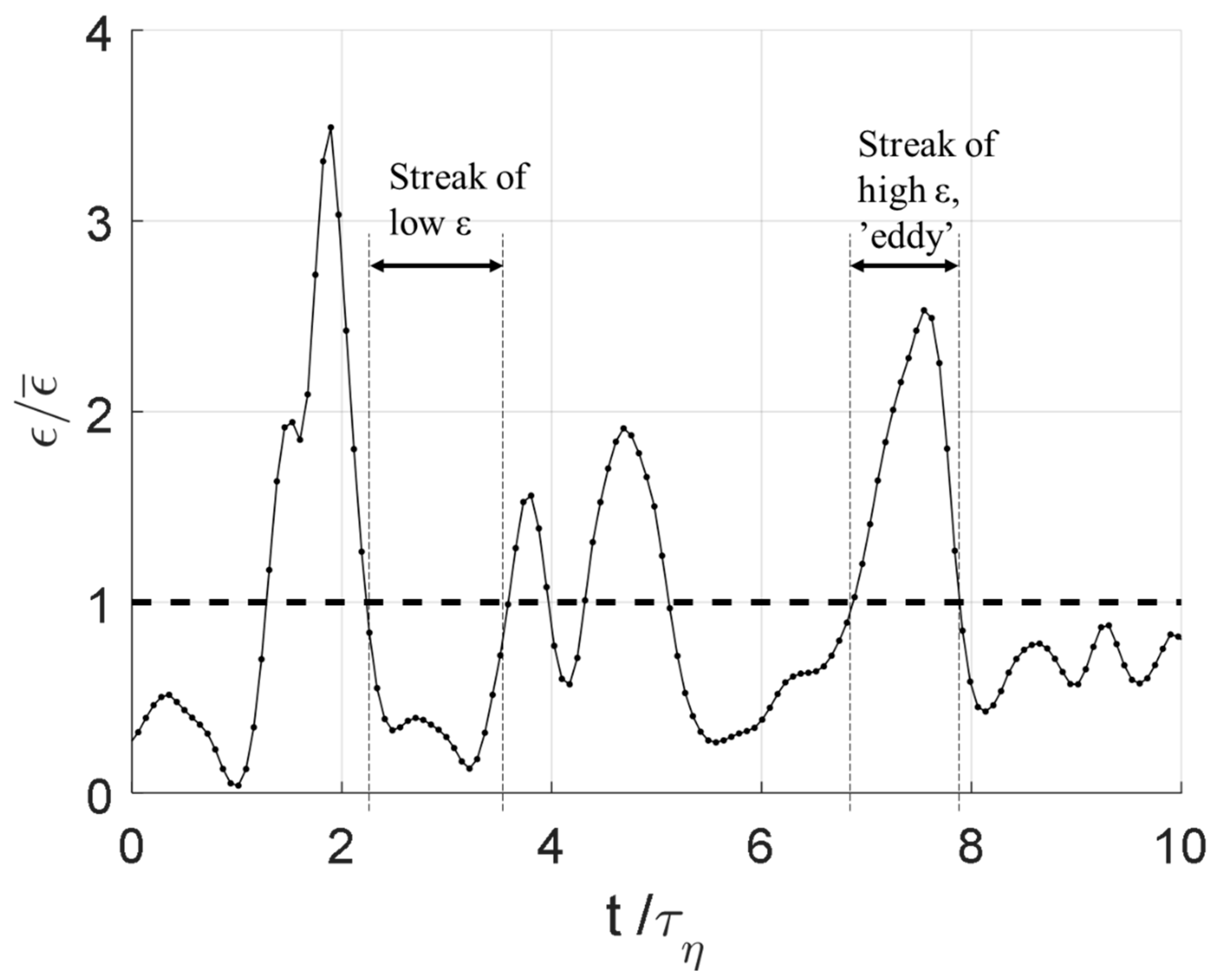
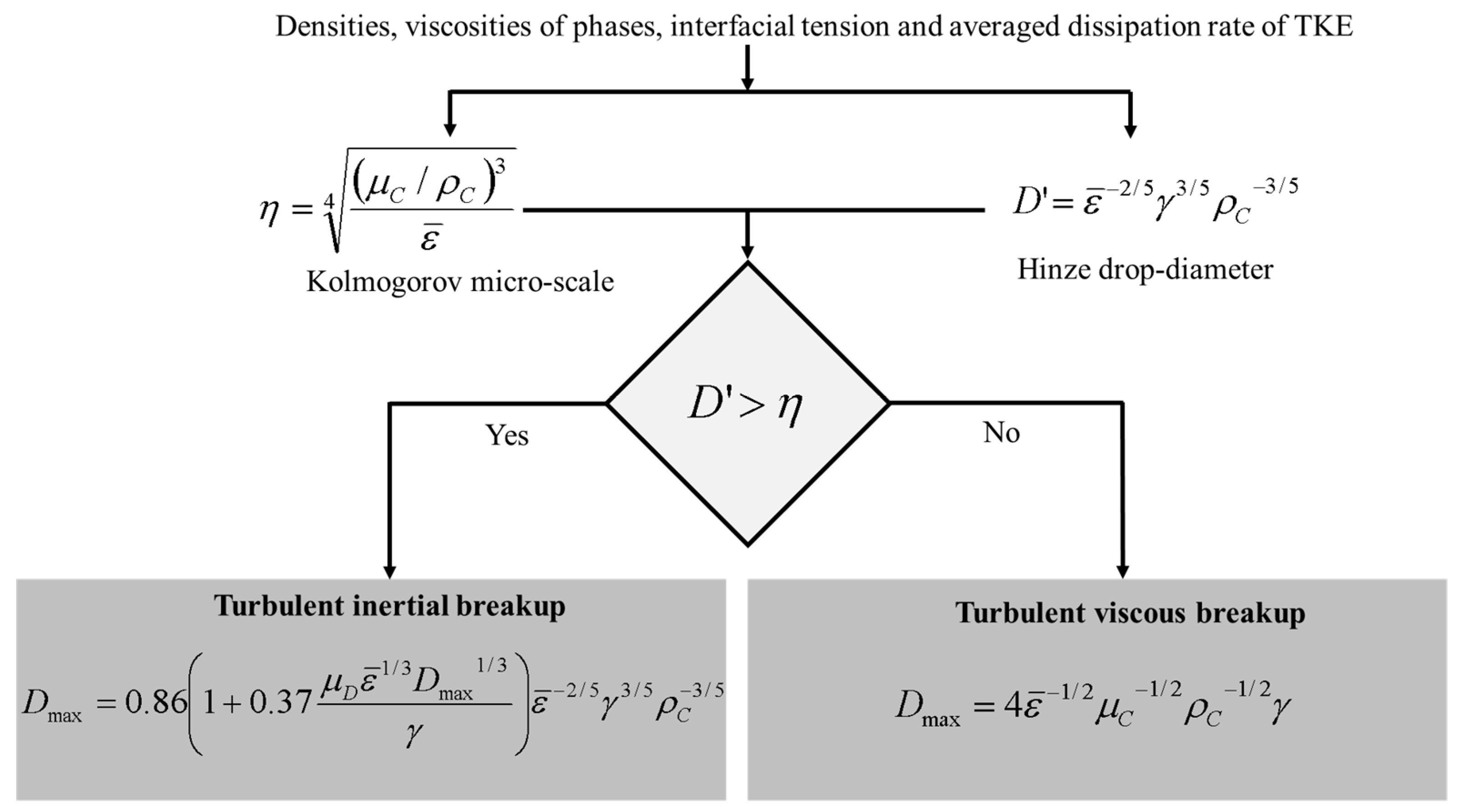
• Experimental characterization of emulsification devices. As discussed in Section 3, there is substantial literature in the fluid mechanics field, investigating turbulent intermittency effects in general and stochastic time-variations of turbulent stresses in particular (e.g., PDFs of dissipation rate of TKE or PDFs of velocity fluctuations) and discussing how they are best modelled [23,24,25,26,27,28]. These investigations are, however, often performed under conditions designed to be as close as possible to idealized turbulent flows (e.g., homogenous, isotropic developed turbulence at a high Reynolds number). Substantially less has been done on the less ideal turbulent flows in emulsification devices. A better understanding of, for example, the PDF of the dissipation rate of TKE in emulsification devices, and, in particular, if differences exist between designs and/or operating conditions, would help in validating proposed models. Another topic of special interest is the eddy life-time concept discussed in the influential two-condition suggestion for the Kolmogorov–Hinze framework. Direct measurements of the dissipation rate of TKE (and other suggestions for the primary fragmenting quantity) would allow for testing of the proposed expression (Equation (16)).
• Further development of multi-fractal breakup theory. In terms of theoretical consistency and connectivity to turbulence theory, the model based on multi-fractal theory stands out as especially interesting. As discussed in Section 4.3 (and further below), it provides testable predictions that are good starting points for future investigations.
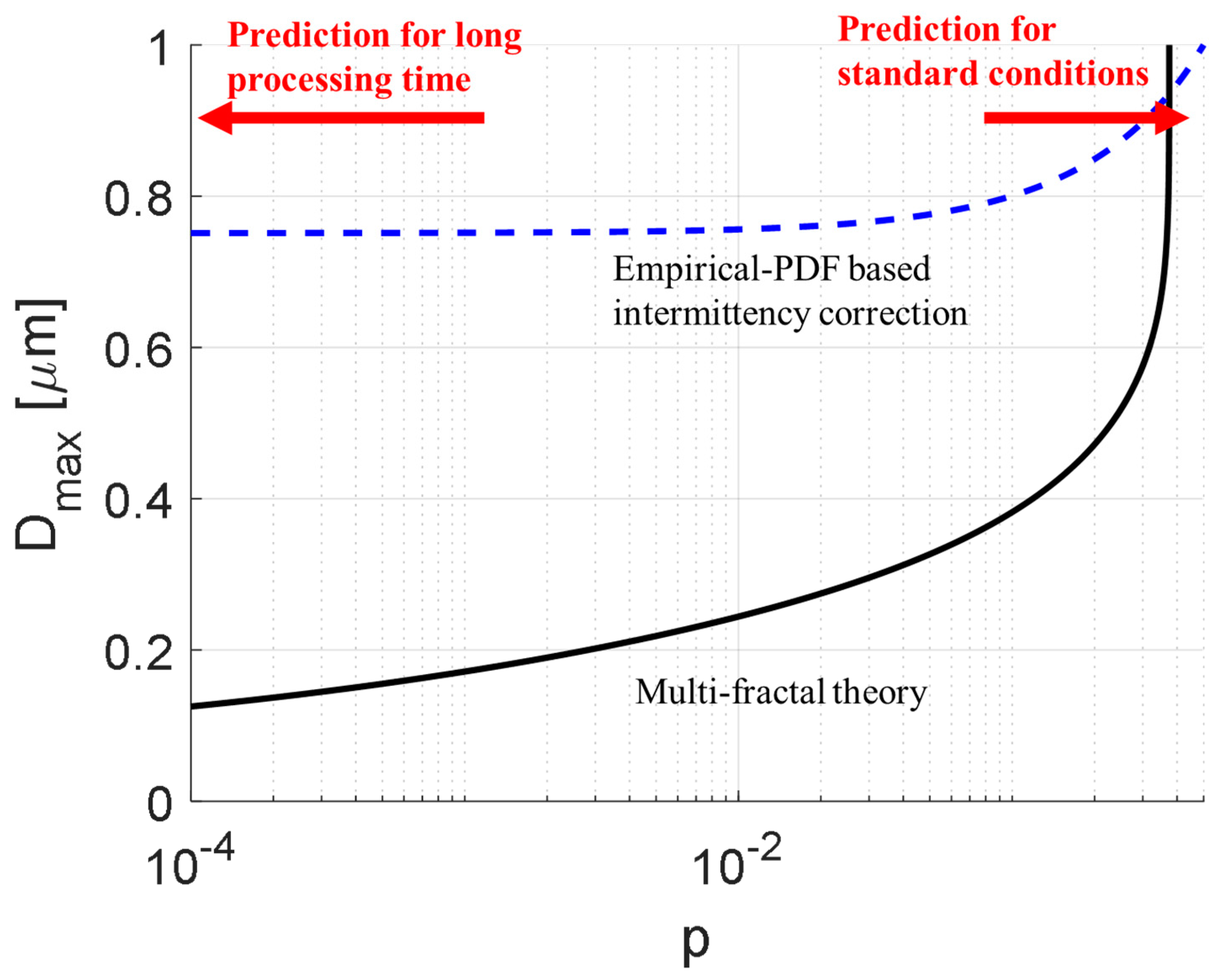
• Long term statistics in emulsification devices. As discussed in Section 4.1, the Kolmogorov–Hinze framework appears to provide relatively good predictions even when neglecting stochastic time-variations altogether. However, there are indications that stochastic time-variations in turbulent stresses start to play a role when attempting to understand and predict differences between multi-pass emulsification in continuous mode of operation devices or emulsification taking place at long processing times in devices operating in the batch mode of operation (see Section 4.5). Measurements of how emulsion size distributions evolve at exceedingly long processing times, compared with the predictions provided by the adaptations reviewed in Section 4.3 and Section 4.4, would be an interesting experimental line of investigation.
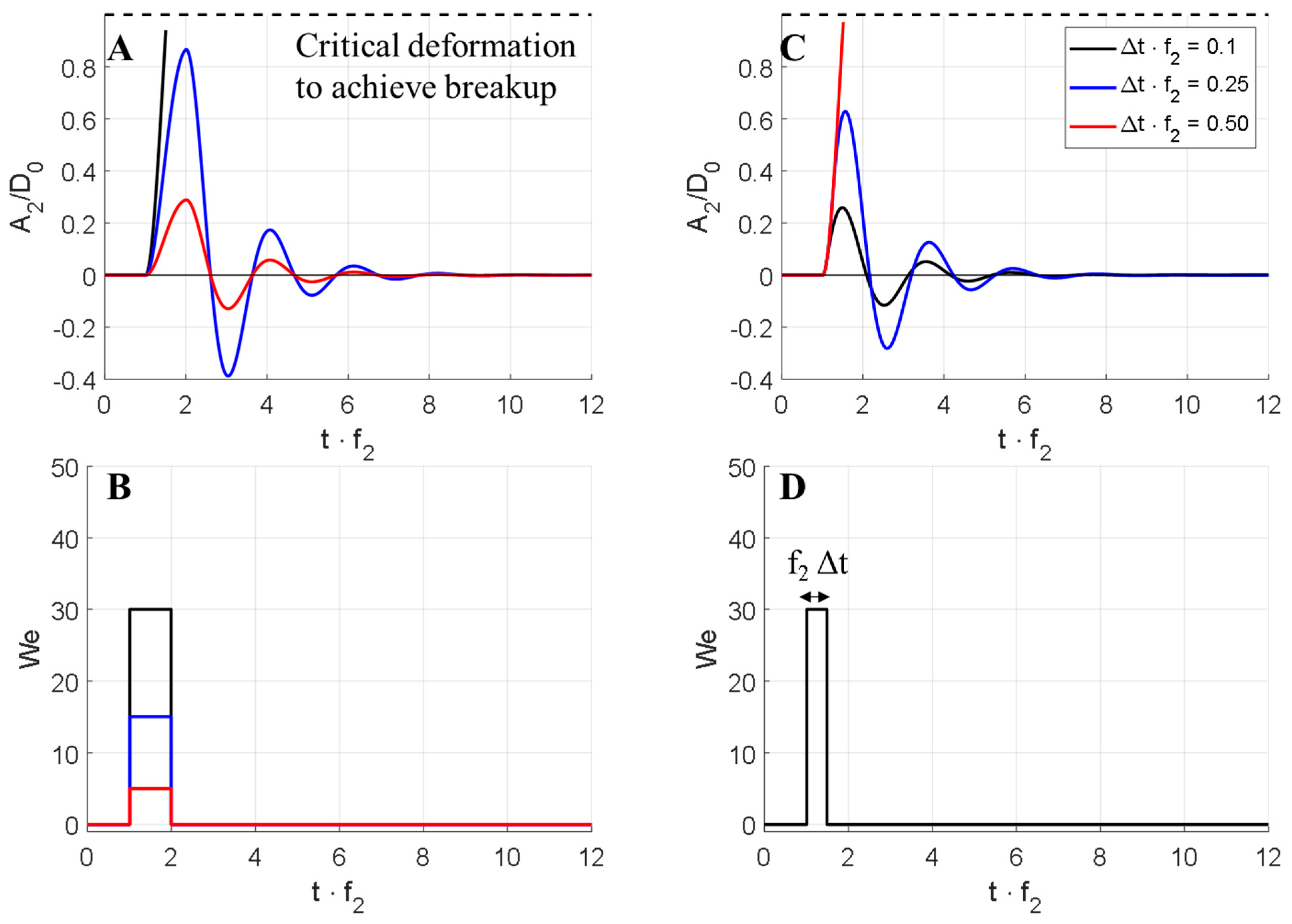
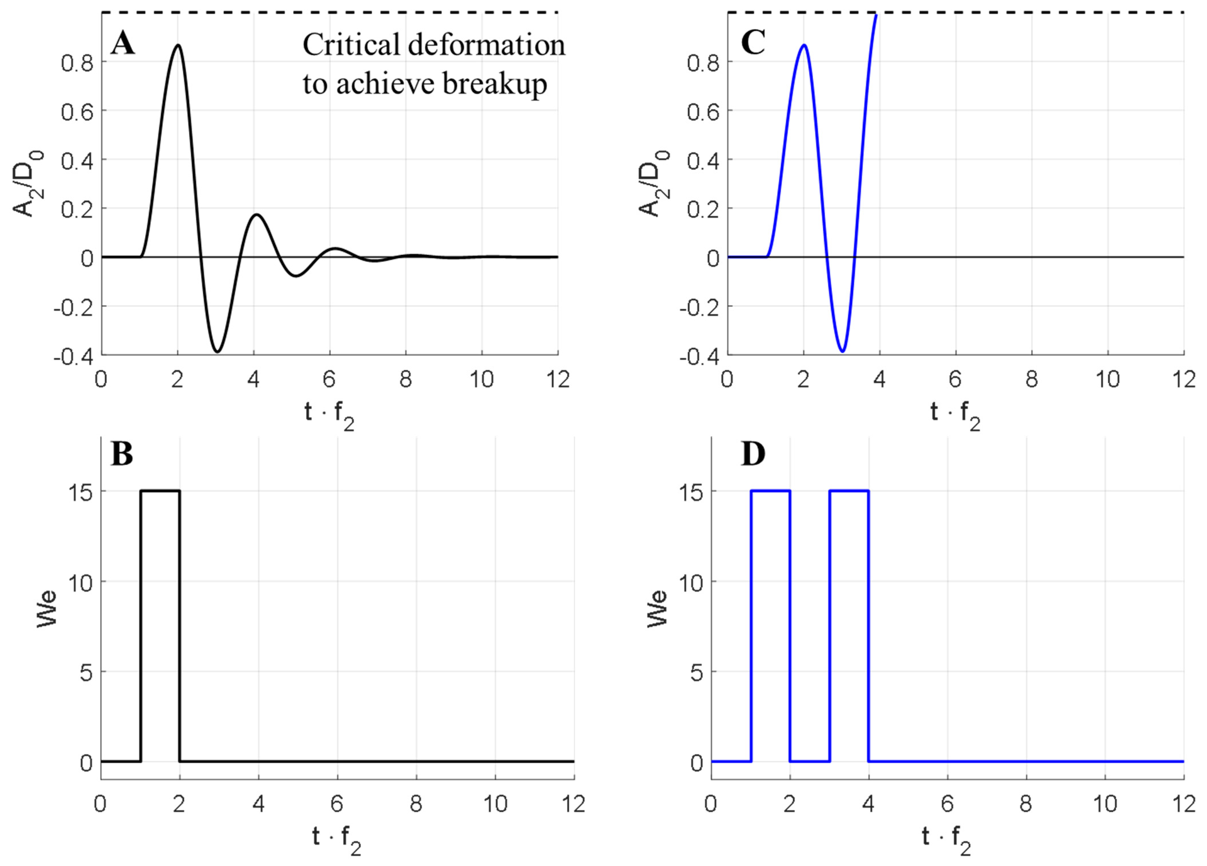
• Application of the oscillatory resonance framework to emulsification devices. The oscillatory resonance framework is an interesting alternative basis for predicting size distributions resulting from emulsification. However, as it is presently formulated, it requires knowledge about the time-history of the local Weber number along the trajectory followed by the drop. This quantity can be measured under carefully controlled experimental conditions [5,18], but is inaccessible for the researcher or engineer working with designing industrial emulsification devices or optimizing processing lines. An extension and development of this framework in order to become applicable to conditions without full knowledge about time-histories (e.g., by combining the Rayleigh–Lamb model in Equation (35) with stochastic process modelling using either multi-fractal theory or purely empirical relationships, cf. Section 4.3 and Section 4.4) would be an interesting theoretical line of investigation.

References

1. Schultz, S.; Wagner, G.; Urban, K.; Ulrich, J. High-pressure homogenization as a process for emulsion formation. Chem. Eng. Technol. 2004, 27, 361–368. [Google Scholar] [CrossRef]
2. Håkansson, A. Emulsion formation by homogenization: Current understanding and future perspectives. Annu. Rev. Food Sci. Technol. 2019, 10, 239–258. [Google Scholar] [CrossRef] [PubMed]
3. Elghobashi, S. Direct numerical simulation of turbulent flows laden with droplets or bubbles. Annu. Rev. Fluid Mech. 2019, 51, 217–244. [Google Scholar] [CrossRef] [Green Version]
4. Rivière, A.; Mostert, W.; Perrard, S.; Deike, L. Sub-Hinze scale bubble production in turbulent bubble break-up. J. Fluid Mech. 2021, 917, 40. [Google Scholar] [CrossRef]
5. Risso, F.; Fabre, J. Oscillations and breakup of a bubble immersed in a turbulent field. J. Fluid Mech. 1998, 372, 323–355. [Google Scholar] [CrossRef]
6. Qian, D.; McLaughlin, J.B.; Sankaranarayanan, K.; Sundaresan, S.; Kontomaris, K. Simulation of bubble breakup dynamics in homogeneous turbulence. Chem. Eng. Commun. 2006, 193, 1038–1063. [Google Scholar] [CrossRef]
7. Kolmogorov, A.N. On the breakage of drops in a turbulent flow. Dokl. Akad. Nauk. SSSR 1949, 66, 825–828. [Google Scholar]
8. Hinze, J.O. Fundamentals of the hydrodynamic mechanism of splitting in dispersion processes. AIChE J. 1955, 1, 289–295. [Google Scholar] [CrossRef]
9. Vankova, N.; Tcholakova, S.; Denkov, N.; Ivanov, I.B.; Vulchev, V.; Danner, T. Emulsification in turbulent flow. J. Colloid Interface Sci. 2007, 312, 363–380. [Google Scholar] [CrossRef]
10. Boxall, J.A.; Koh, C.A.; Sloan, E.D.; Sum, A.; Wu, D.T. Droplet size scaling of water-in-oil emulsions under turbulent flow. Langmuir 2012, 28, 104–110. [Google Scholar] [CrossRef] [PubMed]
11. Calabrese, R.V.; Chang, T.P.K.; Dang, P.T. Drop breakup in turbulent stirred-tank contactors. Part I: Effect of dispersed-phase viscosity. AIChE J. 1986, 32, 657–666. [Google Scholar] [CrossRef] [Green Version]
12. Ramkrishna, D. Population Balances–Theory and Applications to Particulate Systems in Engineering; Academic Press: San Diego, CA, USA, 2000. [Google Scholar]
13. Ramkrishna, D.; Singh, M.R. Population balance modeling: Current status and future prospects. Annu. Rev. Chem. Biomol. Eng. 2014, 5, 123–146. [Google Scholar] [CrossRef] [Green Version]
14. Coulaloglou, C.; Tavlarides, L. Description of interaction processes in agitated liquid-liquid dispersions. Chem. Eng. Sci. 1977, 32, 1289–1297. [Google Scholar] [CrossRef]
15. Solsvik, J.; Tangen, S.; Jakobsen, H.A. On the constitutive equations for fluid particle breakage. Rev. Chem. Eng. 2013, 29, 241–356. [Google Scholar] [CrossRef]
16. Liao, Y.; Lucas, D. A literature review of theoretical models for drop and bubble breakup in turbulent dispersions. Chem. Eng. Sci. 2009, 64, 3389–3406. [Google Scholar] [CrossRef]
17. Lalanne, B.; Masbernat, O.; Risso, F. A model for drop and bubble breakup frequency based on turbulence spectra. AIChE J. 2018, 65, 347–359. [Google Scholar] [CrossRef] [Green Version]
18. Galinat, S.; Risso, F.; Masbernat, O.; Guiraud, P. Dynamics of drop breakup in inhomogeneous turbulence at various volume fractions. J. Fluid Mech. 2007, 578, 85–94. [Google Scholar] [CrossRef]
19. Walstra, P. Emulsions. In Fundamentals of Interface and Colloid Science; Lyklema, J., Ed.; Elsevier: Amsterdam, The Netherlands, 2005; pp. 81–94. [Google Scholar]
20. Li, Y.; Perlman, E.; Wan, M.; Yang, Y.; Meneveau, C.; Burns, R.; Chen, S.; Szalay, A.; Eyink, G. A public turbulence database cluster and applications to study Lagrangian evolution of velocity increments in turbulence. J. Turbul. 2008, 9, N31. [Google Scholar] [CrossRef] [Green Version]
21. Perlman, E.; Burns, R.; Li, Y.; Meneveau, C. Data exploration of turbulence simulations using a database cluster. In Proceedings of the 2007 ACM/IEEE conference on Supercomputing-SC ’07, Reno, NV, USA, 10–16 November 2007. [Google Scholar]
22. Graham, J.; Kanov, K.; Yang, X.I.A.; Lee, M.; Malaya, N.; Lalescu, C.C.; Burns, R.; Eyink, G.; Szalay, A.; Moser, R.; et al. A Web services accessible database of turbulent channel flow and its use for testing a new integral wall model for LES. J. Turbul. 2016, 17, 181–215. [Google Scholar] [CrossRef]
23. Kolmogorov, A.N. A refinement of previous hypotheses concerning the local structure of turbulence in a viscous incompressible fluid at high Reynolds number. J. Fluid Mech. 1962, 13, 82–85. [Google Scholar] [CrossRef] [Green Version]
24. Obukhov, A.M. Some specific features of atmospheric turbulence. J. Geophys. Res. Space Phys. 1962, 67, 3011–3014. [Google Scholar] [CrossRef]
25. Gurvich, A.S. Breakdown of Eddies and probability distributions for small-scale turbulence. Phys. Fluids 1967, 10, S59. [Google Scholar] [CrossRef]
26. Jimenez, J. Small scale intermittency in turbulence. Eur. J. Mech. B Fluids 1998, 17, 405–419. [Google Scholar] [CrossRef]
27. Lohse, D.; Grossmann, S. Intermittency in turbulence. Phys. A Stat. Mech. Appl. 1993, 194, 519–531. [Google Scholar] [CrossRef]
28. Pope, S.B. Turbulent Flows; Cambridge University Press: Cambridge, UK, 2000. [Google Scholar]
29. Batchelor, G.K.; Townsend, A.A. The nature of turbulent motion at large wave-numbers. Proc. R. Soc. London. Ser. A Math. Phys. Sci. 1949, 199, 238–255. [Google Scholar] [CrossRef]
30. Tcholakova, S.; Denkov, N.D.; Lips, A. Comparison of solid particles, globular proteins and surfactants as emulsifiers. Phys. Chem. Chem. Phys. 2008, 10, 1608–1627. [Google Scholar] [CrossRef]
31. Gupta, A.; Eral, H.B.; Hatton, T.A.; Doyle, P.S. Controlling and predicting droplet size of nanoemulsions: Scaling relations with experimental validation. Soft Matter 2016, 12, 1452–1458. [Google Scholar] [CrossRef] [Green Version]
32. Shinnar, R. On the behaviour of liquid dispersions in mixing vessels. J. Fluid Mech. 1961, 10, 259–275. [Google Scholar] [CrossRef]
33. Taylor, G.I. The formation of emulsions in definable fields of flow. In Royal Society of London. A. Mathematical and Physical Sciences; The Royal Society: London, UK, 1934; Volume 146, pp. 501–523. [Google Scholar]
34. Grace, H.P. Dispersion phenomena in high viscosity immiscible fluid systems and application of static mixers as dispersion devices in such systems. Chem. Eng. Commun. 1982, 14, 225–277. [Google Scholar] [CrossRef]
35. Higdon, J.J.L. The kinematics of the four-roll mill. Phys. Fluids A Fluid Dyn. 1993, 5, 274–276. [Google Scholar] [CrossRef]
36. Innings, F.; Hamberg, L.; Trägårdh, C. Dynamic modelling of the deformation of a drop in a four-roll mill. Chem. Eng. Sci. 2005, 60, 4771–4779. [Google Scholar] [CrossRef]
37. Feigl, K.; Kaufmann, S.F.; Fischer, P.; Windhab, E.J. A numerical procedure for calculating droplet deformation in dispersing flows and experimental verification. Chem. Eng. Sci. 2003, 58, 2351–2363. [Google Scholar] [CrossRef]
38. Windhab, E.; Dressler, M.; Feigl, K.; Fischer, P.; Megias-Alguacil, D. Emulsion processing—from single-drop deformation to design of complex processes and products. Chem. Eng. Sci. 2005, 60, 2101–2113. [Google Scholar] [CrossRef]
39. Stone, H.A.; Bentley, B.J.; Leal, L.G. An experimental study of transient effects in the breakup of viscous drops. J. Fluid Mech. 1986, 173, 131–158. [Google Scholar] [CrossRef] [Green Version]
40. Rallison, J.M. The deformation of small viscous drops and bubbles in shear flows. Annu. Rev. Fluid Mech. 1984, 16, 45–66. [Google Scholar] [CrossRef]
41. Stone, A.H. Dynamics of drop deformation and breakup in viscous fluids. Annu. Rev. Fluid Mech. 1994, 26, 65–102. [Google Scholar] [CrossRef]
42. Davidson, P. Turbulence. An Introduction for Scientists and Engineers; Oxford University Press: Oxford, UK, 2015. [Google Scholar]
43. Tennekes, H.; Lumley, J.L. A First Course in Turbulence; The MIT Press: Cambridge, MA, USA, 1972. [Google Scholar]
44. Batchelor, G.K. The Theory of Homogeneous Turbulence; Cambridge University Press: Cambridge, UK, 1953. [Google Scholar]
45. White, F.G. Fluid Mechanics, 4th ed.; McGraw-Hill: Boston, MA, USA, 1998. [Google Scholar]
46. Wang, G.; Yang, F.; Wu, K.; Ma, Y.; Peng, C.; Liu, T.; Wang, L.-P. Estimation of the dissipation rate of turbulent kinetic energy: A review. Chem. Eng. Sci. 2021, 229, 116133. [Google Scholar] [CrossRef]
47. Goto, S.; Vassilicos, J.C. The dissipation rate coefficient of turbulence is not universal and depends on the internal stagnation point structure. Phys. Fluids 2009, 21, 035104. [Google Scholar] [CrossRef]
48. Vassilicos, J.C. Dissipation in turbulent flows. Annu. Rev. Fluid Mech. 2015, 47, 95–114. [Google Scholar] [CrossRef] [Green Version]
49. Narsimhan, G.; Gupta, J.; Ramkrishna, D. A model for transitional breakage probability of droplets in agitated lean liquid-liquid dispersions. Chem. Eng. Sci. 1979, 34, 257–265. [Google Scholar] [CrossRef]
50. Perlekar, P.; Biferale, L.; Sbragaglia, M.; Srivastava, S.; Toschi, F. Droplet size distribution in homogeneous isotropic turbulence. Phys. Fluids 2012, 24, 65101. [Google Scholar] [CrossRef] [Green Version]
51. Solsvik, J.; Jakobsen, H.A. A review of the statistical turbulence theory required extending the population balance closure models to the entire spectrum of turbulence. AIChE J. 2016, 62, 1795–1820. [Google Scholar] [CrossRef]
52. Batchelor, G.K. Pressure fluctuations in isotropic turbulence. Math. Proc. Camb. Philos. Soc. 1951, 47, 359–374. [Google Scholar] [CrossRef]
53. Karimi, M.; Andersson, R. Stochastic simulation of droplet breakup in turbulence. Chem. Eng. J. 2020, 380, 122502. [Google Scholar] [CrossRef]
54. Tavoularis, S.; Corrsin, S. Experiments in nearly homogenous turbulent shear flow with a uniform mean temperature gradient. Part 1. J. Fluid Mech. 1981, 104, 311–347. [Google Scholar] [CrossRef] [Green Version]
55. Vejražka, J.; Zednikova, M.; Stanovsky, P. Experiments on breakup of bubbles in a turbulent flow. AIChE J. 2017, 64, 740–757. [Google Scholar] [CrossRef]
56. Jung, S.; Swinney, H.L. Velocity difference statistics in turbulence. Phys. Rev. E 2005, 72, 026304. [Google Scholar] [CrossRef] [Green Version]
57. Lozovatsky, I.; Fernando, H.J.S.; Planella-Morato, J.; Liu, Z.; Lee, J.-H.; Jinadasa, S.U.P. Probability distribution of turbulent kinetic energy dissipation rate in ocean: Observations and approximations. J. Geophys. Res. Oceans 2017, 122, 8293–8308. [Google Scholar] [CrossRef]
58. Lozovatsky, I.; Shearman, K.; Pirro, A.; Fernando, H.J.S. Probability distribution of turbulent kinetic energy dissipation rate in stratified turbulence: Microstructure measurements in the Southern California Bight. J. Geophys. Res. Oceans 2019, 124, 4591–4604. [Google Scholar] [CrossRef]
59. Saddoughi, S.G.; Veeravalli, S.V. Local isotropy in turbulent boundary layers at high Reynolds number. J. Fluid Mech. 1994, 268, 333–372. [Google Scholar] [CrossRef]
60. Davies, J. Drop sizes of emulsions related to turbulent energy dissipation rates. Chem. Eng. Sci. 1985, 40, 839–842. [Google Scholar] [CrossRef]
61. Arai, K.; Konno, M.; Matunaga, Y.; Saito, S. Effect of dispersed-phase viscosity on the maximum stable drop size for breakup in turbulent flow. J. Chem. Eng. Jpn. 1977, 10, 325–330. [Google Scholar] [CrossRef] [Green Version]
62. Babler, M.U.; Biferale, L.; Brandt, L.; Feudel, U.; Guseva, K.; Lanotte, A.S.; Marchioli, C.; Picano, F.; Sardina, G.; Soldati, A.; et al. Numerical simulations of aggregate breakup in bounded and unbounded turbulent flows. J. Fluid Mech. 2015, 766, 104–128. [Google Scholar] [CrossRef] [Green Version]
63. Håkansson, A. Scale-down failed–Dissimilarities between high-pressure homogenizers of different scales due to failed mechanistic matching. J. Food Eng. 2017, 195, 31–39. [Google Scholar] [CrossRef]
64. Walstra, P. Effect of homogenization on the fat globule size distribution in milk. Neth. Milk Dairy J. 1975, 29, 279–294. [Google Scholar]
65. Walstra, P. Principles of emulsion formation. Chem. Eng. Sci. 1993, 48, 333–349. [Google Scholar] [CrossRef]
66. Rayner, M. Scales and forces in emulsification. In Engineering Aspects of Food Emulsification and Homogenization; Rayner, M., Dejmek, P., Eds.; CRC Press: Boca Raton, FL, USA, 2015; pp. 3–32. [Google Scholar]
67. McClements, D.J. Food Emulsions: Principles, Practices, and Techniques; CRC Press: Boca Raton, FL, USA, 2016. [Google Scholar]
68. Casoli, P.; Vacca, A.; Berta, G.L. A numerical procedure for predicting the performance of high pressure homogenizing valves. Simul. Model. Pr. Theory 2010, 18, 125–138. [Google Scholar] [CrossRef]
69. Baldyga, J.; Bourne, J. Some consequences for turbulent mixing of fine-scale intermittency. Chem. Eng. Sci. 1992, 47, 3943–3948. [Google Scholar] [CrossRef]
70. Bałyga, J.; Bourne, J. Interpretation of turbulent mixing using fractals and multifractals. Chem. Eng. Sci. 1995, 50, 381–400. [Google Scholar] [CrossRef]
71. Baldyga, J.; Podgórska, W. Drop break-up in intermittent turbulence: Maximum stable and transient sizes of drops. Can. J. Chem. Eng. 1998, 76, 456–470. [Google Scholar] [CrossRef]
72. Mandelbrot, B.B. Intermittent turbulence in self-similar cascades: Divergence of high moments and dimension of the carrier. J. Fluid Mech. 1974, 62, 331–358. [Google Scholar] [CrossRef]
73. Meneveau, C.; Sreenivasan, K.R. The multifractal nature of turbulent energy dissipation. J. Fluid Mech. 1991, 224, 429–484. [Google Scholar] [CrossRef]
74. Håkansson, A.; Andersson, R.; Mortensen, H.-H.; Innings, F. Experimental investigations of turbulent fragmenting stresses in a rotor-stator mixer. Part 2. Probability distributions of instantaneous stresses. Chem. Eng. Sci. 2017, 171, 638–649. [Google Scholar] [CrossRef]
75. Håkansson, A. An experimental investigation of the probability distribution of turbulent fragmenting stresses in a high-pressure homogenizer. Chem. Eng. Sci. 2018, 177, 139–150. [Google Scholar] [CrossRef]
76. Sheng, J.; Meng, H.; Fox, R. A large eddy PIV method for turbulence dissipation rate estimation. Chem. Eng. Sci. 2000, 55, 4423–4434. [Google Scholar] [CrossRef]
77. Saarenrinne, P.; Piirto, M. Turbulent kinetic energy dissipation rate estimation from PIV velocity vector fields. Exp. Fluids 2000, 29, S300–S307. [Google Scholar] [CrossRef]
78. Tanaka, T.; Eaton, J.K. A correction method for measuring turbulence kinetic energy dissipation rate by PIV. Exp. Fluids 2007, 42, 893–902. [Google Scholar] [CrossRef]
79. Hall, S.; Pacek, A.W.; Kowalski, A.J.; Cooke, M.; Rothman, D. The effect of scale and interfacial tension on liquid–liquid dispersion in in-line Silverson rotor–stator mixers. Chem. Eng. Res. Des. 2013, 91, 2156–2168. [Google Scholar] [CrossRef] [Green Version]
80. De Hert, S.C.; Rodgers, T. Continuous, recycle and batch emulsification kinetics using a high-shear mixer. Chem. Eng. Sci. 2017, 167, 265–277. [Google Scholar] [CrossRef]
81. Håkansson, A.; Chaudhry, Z.; Innings, F. Model emulsions to study the mechanism of industrial mayonnaise emulsification. Food Bioprod. Process 2016, 98, 189–195. [Google Scholar] [CrossRef]
82. Lamb, H. Hydrodynamics, 6th ed.; Cambridge University Press: Cambridge, UK, 1932. [Google Scholar]
83. Jafari, S.; McClements, D.J. Nanoemulsions: Formulation, Applications, and Characterization; Academic Press: Cambridge, MA, USA, 2018. [Google Scholar]
Figure 1. The instantaneous dissipation rate of TKE (ε), as a function of time (t) in a pipe flow at a position in the proximity of the wall (y+ = 90). The horizontal axis is normalized by the time-averaged value, ε ¯ (obtained over a time substantially longer than the displayed interval) and the horizontal axis is normalized with the Kolmogorov time-scale, τη. (Calculated based on DNS-generated raw data for a turbulent channel with a bulk Reynolds number of 40,000 from the John Hopkins Turbulence Database, DOI: 10.7281/T10K26QW).
Processes 09 01904 g001
Figure 2. Schematically illustration of laminar breakup in a four-roller mill [33,35]: (A) The four-roller mill; (B) the laminar velocity profiles (with streamlines); (C) schematic illustration of the laminar shear experienced by a drop placed in the flow.
Processes 09 01904 g002
Figure 3. Illustration of the instantaneous flow in a channel with developed turbulence; (A) velocity magnitude of instantaneous stream-wise velocities in a subsection of the channel (wall at y = −1, y = 0 represents the center axis); (B) stream-wise velocity profiles in the channel, showing the instantaneous velocities at three randomly chosen points in time (black, red and blue dots) and the time-averaged velocity according to Prandtl’s 1/7th power law (dashed line).
Processes 09 01904 g003
Figure 4. Flowchart representation of the drop-viscosity-corrected Kolmogorov–Hinze framework (freely after the algorithmic interpretation first suggested in [9]).
Processes 09 01904 g004
Figure 5. Maximum drop diameter according to the two-criterion extension (Equation (18)) (solid black line) compared to that of the viscosity-stabilization corrected Kolmogorov–Hinze theory (Equation (11)) (dotted red line) as a function of viscosity ratio (μD/μC).
Processes 09 01904 g005
Figure 6. Illustration of multi-fractal model; (A) Bałdyga and Bourne’s [70] suggestion for the PDF of the eddy labelling dimension α; (B) the instantaneous stress normalized to its time-averaged value (Equation (18)), as a function of the labelling dimension α; (C) the resulting PDF of disruptive stress, obtained by combining (A,B).
Processes 09 01904 g006
Figure 7. Prediction of maximum drop diameter, Dmax, for the case of a highly viscous drop in water as a function of time-averaged dissipation rate of TKE, ε ¯ . Predictions are shown for the traditional Kolmogorov–Hinze framework neglecting stochastic time-variations in turbulent stresses (α = 1, Figure 4) and for the multifractal correction (Equation (21)), for exceedingly long processing times (α = 0.12).
Processes 09 01904 g007
Figure 8. Experimentally measured PDF of instantaneous stresses calculated from particle image velocimetry results in the efficient region of breakup in a HPH geometry (black disks) [75] and in a batch RMS [74] operating at either 333 rpm (blue disks) or 1233 rpm (blue squares). Solid line: lognormal pdf with q = 0.34.
Processes 09 01904 g008
Figure 9. Comparing the predicted maximum drop diameter between the multi-fractal suggestion (Section 4.3) and the empirical-PDF based suggestion (Section 4.4), as a function of the limiting probability p required for having an instantaneous stress exceeding the stabilizing stress. Values of p ~ 1 correspond to cases where the drop spends a relatively short time-period in the turbulence (and thus only instantaneous stresses that occur with a high probability play a role) whereas p → 0 corresponds to when the drop spends a very long period of time in the turbulence (and thus even an instantaneous stress that only occurs with a low probability will play a role).
Processes 09 01904 g009
Figure 10. The number, n, of passages through a breakup region required to achieve a reduction of the maximum drop diameter Dmax by a factor 1:10, as a function of x, the drop volume fraction ending up in the largest fragment (Equation (32)).
Processes 09 01904 g010
Figure 11. Illustration of the Rayleigh–Lamb model (Equation (35)), showing how the drop amplitude behaves when encountering a single high-We pulse with a duration Δt. The drop is predicted to break once the deformation reaches A2/D0 = 1 (i.e., when extended to a length equal to twice the initial diameter); (A,B) compare three cases where the drop is subjected to a fixed width pulse (f2 Δt = 1) with different intensities (We = 30, black; We = 15, blue and We = 5, red); (C,D) compare three cases with constant pulse intensity (We = 30) but different pulse widths (f2 Δt = 0.1, black; f2 Δt = 0.25, blue and f2 Δt = 0.5, red). (D0 = 50 µm, ρC = ρD =103 kg/m3, μC = μD = 1 mPa s, γ = 20 mN/m and K = 1/25.)
Processes 09 01904 g011
Figure 12. Illustration of the Rayleigh–Lamb model (Equation (35)), showing the effect of a sequence of eddies; (A,B) show how the drop amplitude behaves when encountering a single high-We pulse (We = 15) with a duration (f2 Δt = 1); (C,D) show how the drop amplitude behaves when encountering two successive pulses separated by a time Δt. (Settings as in Figure 11.)
Processes 09 01904 g012
Publisher’s Note: MDPI stays neutral with regard to jurisdictional claims in published maps and institutional affiliations.