Carbon-Efficient Production Scheduling of a Bioethanol Plant Considering Diversified Feedstock Pelletization Density: A Case Study

Abstract

This paper presents a dual-objective optimization model for production scheduling of bioethanol plant with carbon-efficient strategies. The model is developed throughout the bioethanol production process. Firstly, the production planning and scheduling of the bioethanol plant’s transportation, storage, pretreatment, and ethanol manufacturing are fully considered. Secondly, the carbon emissions in the ethanol manufacturing process are integrated into the model to form a dual-objective optimization model that simultaneously optimizes the production plan and carbon emissions. The effects of different biomass raw materials with optional pelletization density and pretreatment methods on production scheduling are analyzed. The influence of demand and pretreatment cost on selecting a pretreatment method and total profit is considered. A membership weighted method is developed to solve the dual-objective model. The carbon emission model and economic model are integrated into one model for analysis. An example is given to verify the effectiveness of the optimization model. At the end of the paper, the limitation of this study is discussed to provide directions for future research.

1. Introduction

With the growing concerns on the aggravated global climate problem, more attention is paid to exploit clean energy. In 2019, the production of transportation biofuels increased by 6% year-on-year, and annual production is expected to increase by 3% in the next 5 years. China plans to introduce a mixture of 10% ethanol in gasoline from 11 to 15 provinces, and new ethanol production capacity is under development [1]. In addition, biofuels have become popular due to the wide range of sources of biomass raw materials and lower manufacturing costs. Bioethanol is one of the most common biofuels. Bioethanol as a biofuel can replace fossil energy well to reduce the harm to the environment. Bioethanol faces challenges such as production technology, transportation, and raw material supply in the production process [2,3]. Additionally, the production of bioethanol is closely connected with agricultural production dealing with surplus crop straws, which contributes to increasing farmers’ incomes. As a result, United States, Brazil, China, etc., have established biofuel production plants, which promote resource recycling and environmental protection of agricultural, forestry, urban and rural organic waste, and save the use of non-renewable energy.

Every country has set biofuel development goals and provided incentives and support to accelerate the development of the biofuel industry. Currently, wheat or corn can be used as raw materials for biofuel plants to produce bioethanol [4,5]. Food prices are likely to rise as demand for grain increases [6]. In order to reduce the adverse impact on food security, the government encourages to increase the utilization proportion of non-food biomass raw materials. The production of bioethanol will be well developed in the future. Therefore, how to organize the production and logistics to take full advantage of bioenergy resources is crucial, from the aspect of either supply chain or manufacturing. Especially for sustainable development, supply chain network design and logistics problems throughout the whole production and transportation process should be conducted [7,8].

Due to the serious environmental pollution caused by the use of traditional energy, renewable energy met approximately 3.7% of transportation fuel demand in 2018. In 2018, global biofuel production increased by 10 billion liters, reaching a record 154 billion liters [9]. Since biofuels play an important role, the impact of carbon emissions on the production and transportation of bioethanol is considered to effectively reduce carbon emissions.

Most scholars in this field focus on strategic design and tactical optimization at the supply chain level [10,11]. However, there are complex and customized processes in factory production. For example, the storage and processing of biomass raw materials in the bioethanol manufacturing process, the selection of biomass raw materials saccharification process, the determination of bioethanol fermentation quantity, etc. At present, there are few studies on the operational decision-making and scheduling of the production process for bioethanol plants. Additionally, there is a lack of decision tool to simultaneously control the production and logistics to achieve a carbon-efficient and beneficial goal. This paper presents a specific carbon-efficient production scheduling optimization model for the bioethanol plant, and proposes a dual-objective optimization approach to demonstrate the effectiveness on flexible decisions between carbon emission and profit. The effects of different biomass raw materials with optional pelletization density and pretreatment methods on production scheduling are analyzed.

The rest of this paper is organized as follows: the related literature is reviewed in Section 2. The proposed problem is described in detail in Section 3, and the detailed mathematical model and the solution method is thereby introduced in Section 4. In Section 5, case study and computational analysis are presented. Finally, the conclusion is reported in Section 6.

2. Literature Review

With the wide application of clean energy and renewable fuels, more research on improving utilization of bioethanol has been undertaken by both academia and industry. Most of the published literature on supply chain research focuses on strategic and tactical decisions [8]. Yue et al. [12] introduced the key issues and challenges facing biomass energy and biofuel supply chain. Giarola et al. [13] used a general mixed integer linear programming (MILP) model framework that supports multi-stage ethanol supply chain strategic design and planning decisions. De Jong et al. [14] optimized biofuel production costs through scale, integration, transportation, and supply chain configuration. Sharma et al. [15] proposed a comprehensive approach to the biofuel supply chain that takes into account the uncertainty of biomass production. Akhtari and Sowlati [16] comprehensively consider the bioenergy and biofuel supply chain, and propose a systematic approach that comprehensively considers strategic, tactical, and operational decisions. Additionally, a hybrid optimization model is proposed to solve the integration problem. Li et al. [17] proposed an optimized model for the production of bioethanol from cellulose crops and food. The economic cost and carbon emission cost of the biofuel supply chain are studied. Roni et al. [18] presents a distributed supply chain approach to deal with the problem of overwide distribution of biomass raw materials and high transportation costs of biomass raw materials. Biomass raw materials will face various problems in the process of transportation, and the adoption of distributed supply chain can effectively reduce the cost in the process of biomass raw materials supply [14].

Due to the low density of raw materials and the loss during raw material transportation, the cost of raw materials during transportation is too high [19]. To address these issues, the biomass raw materials should be densified before being shipped to the bioethanol plant [20,21]. The most common densification methods of biomass raw materials include packaging, pelleting, etc., which may lead to different biomass density. Densification of biomass is crucial to improve the ethanol yield per unit volume of biomass transportation. Due to high logistics costs and different product yields, optimization decisions provide options to improve utilization. In recent years, researchers proposed MILP models to solve strategic decision-making problems, including the location of bioenergy plants [22,23], and location selection of the biomass raw material collection facilities [24]. On the other hand, the location of a pretreatment warehouse should be considered in the aspect of the pretreatment processing [25]. In particular, considering the process of densification on biomass raw materials, and the diversification of pretreatment sites, Albashabsheh and Heier Stamm [26] put forward the method of making a granulation machine move to optimize the pretreatment and logistics cost.

In addition to the research on raw material warehouse location and raw material pretreatment, the research on production process scheduling has been paid more and more attention. Zhang et al. [27] solved the multi-objective optimization problem of production planning and scheduling problems in the factory production process. Wang et al. [28] proposed a scheduling method that responds to a large number of products and realizes real-time scheduling of workshop products. Georgiadis et al. [29] proposed an efficient MILP-based solution to optimize the weekly schedule of Spanish canned fish production scheduling. In order to reduce the computational complexity, they presented an aggregation method, which modeled the continuous process in detail and introduced effective feasibility constraints for the intermittent phase. Then, two MILP models were established by discrete-continuous mixed time representation. Osmani and Zhang [30] introduced a multi-period bioethanol supply chain under uncertain conditions, to optimize economic and environmental benefits.

With the increasing awareness of environmental protection and sustainability, the study of the green supply chain design and its impacts on the environment was proposed [31]. Li et al. [32] proposed a comprehensive optimization model for the biomass feedstock distribution problem with carbon emission constraint. Cong et al. [33] studied supply chain optimization strategies to reduce carbon emissions under the uncertainty of earnings. Gonela [34] studied random optimization of the hybrid power supply chain with a carbon emission scheme. Zhao et al. [31] established a green supply chain management method relying on big data analysis methods. Lu et al. [35] proposes a comprehensive scheduling of mixed production and recovery systems in a multi-product, carbon-emitting environment. Xu and Wang [36] considered the issue of emission reduction in the supply chain.

Although some work has been done on the design of the bioethanol supply chain network, most of the existing research has focused on strategic decisions such as bioethanol processing site selection or pretreatment. However, there is a lack of research on developing a carbon-efficient production scheduling strategy of the bioethanol plant considering diversified feedstock with optional pelletization density. In order to deal with this problem, this paper first establishes a MILP model of bioethanol production process scheduling considering the trade-off between carbon emissions and profits. Secondly, based on the influence of different pretreatment schemes on bioethanol yield in the process of bioethanol production, the influence of pretreatment schemes on the total profit with varying demand conditions is studied. Finally, a dual-objective optimization approach based on weighted membership is applied to quantitatively balance the effects of carbon emission on the production scheduling, and based on which provides a carbon-efficient tool to design the production scheduling of the bioethanol plant.

3. Problem Description

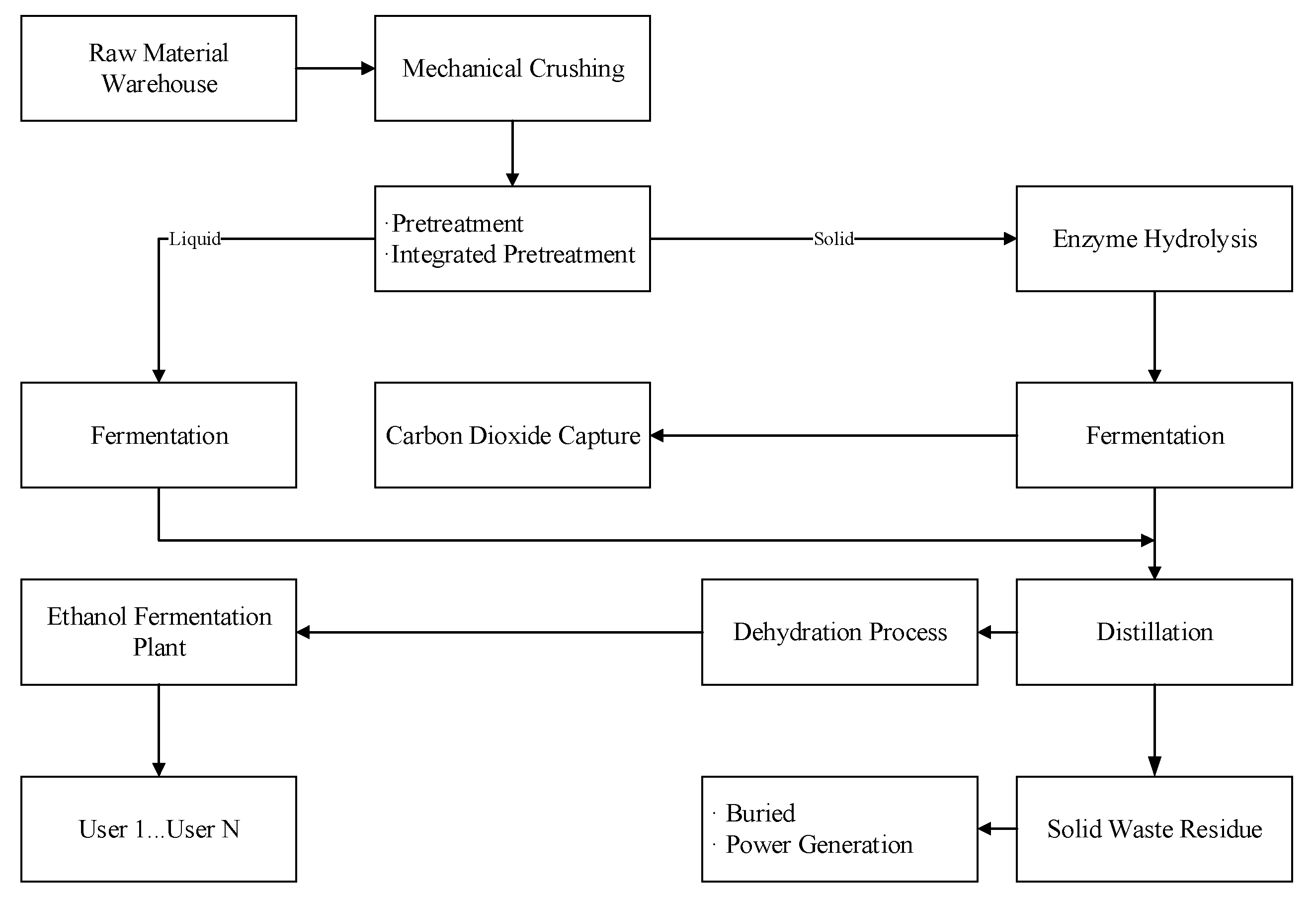
The entire production process of the bioethanol plant is described in Figure 1, that consists of multiple production options and processing route due to the diversified feedstock with optional pelletization density. Different biomass raw materials are packed in different shapes, such as rectangular, round, and pelleted, and are firstly transported to factory warehouses for storage directly or after being crushed. The crushing operation is not only convenient to store, but also facilitates the subsequent operations. The crushed biomass raw materials are transported to a saccharification workshop to transform them into saccharified liquid through several chemical reactions. Then, the produced saccharified liquid is directly transported to the fermentation tank for bioethanol fermentation treatment, or to be stored in the saccharification tank for the subsequent usage. Finally, the saccharified liquid is fermented and transformed into bioethanol. The price of raw materials is affected by factors such as the location of raw materials, the types of raw materials, and the willingness of farmers to plant.

In addition, the production activities throughout the process, including transportation, crushing, fermentation, and the activities connecting upstream and downstream need energy investment, which induces greenhouse gas emissions. Therefore, greenhouse gas emissions should be fully considered in the production process to achieve clean production. For the modeling and solving convenience, the following assumptions are introduced here:

(1)

Transportation costs are only related to packing the biomass raw materials;

(2)

The transportation distances are fixed;

(3)

The supply of raw materials is sufficient in each period.

(4)

The cost of each pretreatment method is only determined by the type of biomass raw materials;

(5)

The price of each raw material is fixed in each period;

(6)

The loss rate of biomass raw materials is fixed, and is only related to the packing forms of the biomass raw materials;

(7)

The loss of the bioethanol storage is negligibly small.

4. Problem Formulation

In this section, the MILP method is used to solve the production scheduling problem of the bioethanol plant. An effective decision-making framework is established by considering the diversity of the biomass raw materials, different raw material pretreatment methods, and bioethanol demand. The planning period is divided into discrete time periods t = 1, ...T, where T is a set of periods within the planning period. Additionally, the duration of each period is 3 days. The subscript indices and sets are defined in

Table 1. Indices.

Notation	Description
$b$	Raw material type, $b\in B$
$j$	Machine, $j\in J$
$k$	Packaging method, $k\in K$
$l$	Biomass raw material warehouse, $l\in L$
$r$	Carbon emission standards, $r\in R$
$t$	Planned periods, $t\in T$
$i$	Preprocessing site, $i\in I$

and

Table 2. Sets.

Notation	Description
$B$	Set of raw material type
$J$	Set of pretreatment machine
$K$	Set of packaging method
$L$	Set of biomass raw material warehouse
$N$	Set of bioethanol warehouse
$R$	Set of carbon emission standards
$T$	Set of planned periods, $t\in T$
$I$	Set of preprocessing site

. Additionally, the model parameters and decision variables are respectively summarized in

Table 3. Parameters.

Parameter	Description
$PE$	Unit price of ethanol
$C{M}_{bk}$	Unit cost of packing method in $b\in B$, $k\in K$
$C{T}_i$	Unit cost of transportation from intermediate goods warehouses to production site
$C{W}_{bkt}$	Unit warehouse storage cost $b\in B$, $k\in K$ at warehouse at period $t\in T$
$C{I}_i$	Unit warehouse storage cost at intermediate goods warehouses
$CE$	Unit ethanol storage cost
$C{R}_r$	Cost of recovering carbon emissions when the carbon emission level is r
$C{B}_i$	Cost per unit of biomass raw material pretreatment
$CP$	Cost per unit of ethanol production
$CM$	Cost per machine
$PM{I}_{bi}$	Price of raw materials type $b\in B$ in intermediate goods warehouses $i\in I$
$P{M}_{bk}$	Price of raw materials with type b and packing method with k
$D_{li}$	Distance from material warehouse l to pretreatment site i
$Q_t$	Demand for bioethanol in each period
${\theta }_{bk}$	Loss rate of raw materials at warehouses
$V_r$	When the carbon emission level is r, $V_r=1$, otherwise $V_r=0$
$W_{bkt}$	The maximum supply of k kinds of $b\in B$, $k\in K$ in period t
${\varphi }_b$	Loss rate of raw materials at warehouses at intermediate goods warehouses
$S_{bk}^{\min }$	Minimum biomass raw material warehouses capacity
$S_{bk}^{\max }$	Maximum biomass raw material warehouses capacity
$Z_{bi}^{\min }$	Minimum capacity of the intermediate product warehouses
$Z_{bi}^{\max }$	Maximum capacity of the intermediate product warehouses
$C^{\min }$	Minimum capacity of an ethanol warehouse
$C^{\max }$	Maximum capacity of an ethanol warehouse
${\gamma }_{bi}$	Ethanol production rate

and

Table 4. Decision variables.

Variable	Description
$A_{bkit}$	Quantity of biomass raw materials transportation to $i$
$P_t$	Bioethanol production at period t
$C_t$	Quantity of storage in the final product warehouses at $t\in T$
$S_{bkt}$	Quantity of raw material stored in the warehouses
$X_{bkt}$	Quantity of biomass raw materials
$Y_{bit}$	Quantity of biomass raw materials in warehouse i to the production workshop
$M_j$	If machine j is operating, $M_j=1$, otherwise $M_j=0$
$Z_{bit}$	Quantity of intermediate goods stored in the warehouses

.

4.1. Objective Function

The aforementioned ethanol biofuel production scheduling problem evaluates two main optimization objectives, they are the total profit and the carbon emission. Since these two aspects are measured by different scale, a dual-objective optimization model is introduced that uses the membership weighting method to solve, and then is optimized simultaneously.

4.1.1. Maximizing the Total Profit

The total profit is obtained by the total sales of ethanol biofuel products minus the operations cost. According to the addressed bioethanol production process, the operations cost mainly includes cost of biomass raw material purchase, biomass raw materials storage, transportation, pretreatment, intermediate product storage, and ethanol fermentation. The objective function is formulated to maximize the total profit.

$${\mathrm{OBJ}}_1=\max (TS-CO)$$

(1)

$$CO=CBR+TCP+TCF+CP+CBP+CSB+CIS+CBS+CRL+CIL+CDG$$

(2)

Total Sales (denoted TS): which is the total sales of the whole production process.

$$TS={\displaystyle \sum _{t\in T}{P}_{t}PE}$$

(3)

Cost of Biomass Procurement (denoted CBR): which is the total cost of procuring the biomass raw materials.

$$CBR={\displaystyle \sum _{b\in B}{\displaystyle \sum _{k\in K}{\displaystyle \sum _{t\in T}{X}_{bkt}P{M}_{bk}}}}$$

(4)

Transportation Costs of the Pretreatment process (denote TCP): which is the cost of transportation from biomass raw material warehouses to the crushing plant.

$$TCP={\displaystyle \sum _{b\in B}{\displaystyle \sum _{k\in K}{\displaystyle \sum _{i=I}{\displaystyle \sum _{t\in T}{\displaystyle \sum _{l\in L}{A}_{bkit}C{M}_{bk}{D}_{li}}}}}}$$

(5)

Transportation Costs of Fermentation (denote TCF): which is the cost of transportation from crushing plant to bioethanol production.

$$TCF={\displaystyle \sum _{b\in B}{\displaystyle \sum _{i=I}{\displaystyle \sum _{t\in T}{Y}_{bit}C{T}_i}}}$$

(6)

Cost of Pretreatment (denote CP): which is the cost of the pretreatment process.

$$CP={\displaystyle \sum _{b\in B}{\displaystyle \sum _{k\in K}{\displaystyle \sum _{i=I}{\displaystyle \sum _{t\in T}{A}_{bkit}C{B}_i}}}}$$

(7)

Cost of bioethanol production (denote CBP): which is the total cost of bioethanol production.

$$CBP={\displaystyle \sum _{b\in B}{\displaystyle \sum _{i=I}{\displaystyle \sum _{t\in T}{Y}_{bit}CP}}}$$

(8)

Cost of Storage Biomass Raw Materials (denote CSB): which is the total cost of biomass raw material storage.

$$CSB={\displaystyle \sum _{b\in B}{\displaystyle \sum _{k\in K}{\displaystyle \sum _{t\in T}{S}_{bkt}C{W}_{bkt}}}}$$

(9)

Cost of Intermediate Warehouse Storage (denote CIS): which is the cost of intermediate goods warehouse storage.

$$CIS={\displaystyle \sum _{b\in B}{\displaystyle \sum _{i=I}{\displaystyle \sum _{t\in T}{Z}_{bit}C{I}_i}}}$$

(10)

Cost of Bioethanol Storage (denote CBS): which is the total storage cost of bioethanol in a bioethanol plant.

$$CBS={\displaystyle \sum _{t\in T}{C}_{t}CE}$$

(11)

Cost of Raw Material Warehouse Loss (denote CRL): which is the loss cost of biomass raw material when stored in a raw material warehouse.

$$CRL={\displaystyle \sum _{b\in B}{\displaystyle \sum _{k\in K}{\displaystyle \sum _{t\in T}{S}_{bkt}P{M}_{bk}{\theta }_{bk}}}}$$

(12)

Cost of Intermediate Warehouse Loss (denote CIL): which is the loss costs incurred in storage of intermediate products in a bioethanol plant.

$$CIL={\displaystyle \sum _{b\in B}{\displaystyle \sum _{i=I}{\displaystyle \sum _{t\in T}{Z}_{bit}{\varphi }_{b}PM{I}_{bi}}}}$$

(13)

Cost of Dealing with Greenhouse (denote CDG): which is the cost of bioethanol plants to deal with carbon emissions.

$$CDG={\displaystyle \sum _{r\in R}C{R}_r{V}_r}$$

(14)

4.1.2. Minimizing the Carbon Emission

Considering the harm caused by the greenhouse gas emission to the environment, controlling the carbon emission has significant environmental value. The bioethanol production process would generate carbon emissions from transportation, pretreatment, the saccharification process, and bioethanol fermentation process. The amount of carbon emissions from the above process is measured by GHG emissions. Therefore, the following function is defined to describe carbon emissions:

$$OB{J}_2=\min (C{E}_1+C{E}_2)$$

(15)

$$\begin{array}{l}C{E}_1={\displaystyle \sum _{b\in B}{\displaystyle \sum _{k\in K}{\displaystyle \sum _{t\in T}{X}_{bkt}E{M}_1}}}+{\displaystyle \sum _{b\in B}{\displaystyle \sum _{k\in K}{\displaystyle \sum _{i=1}{\displaystyle \sum _{t\in T}{A}_{bkit}E{M}_2}}}}+{\displaystyle \sum _{b\in B}{\displaystyle \sum _{k\in K}{\displaystyle \sum _{i=2}{\displaystyle \sum _{t\in T}{A}_{bkit}E{M}_3}}}}+{\displaystyle \sum _{b\in B}{\displaystyle \sum _{i=1}{\displaystyle \sum _{t\in T}{\displaystyle \sum _{r\in R}{Y}_{bit}E{M}_4}}}}\\ \hspace{0.17em}\hspace{0.17em}\hspace{0.17em}\hspace{0.17em}\hspace{0.17em}\hspace{0.17em}\hspace{0.17em}+{\displaystyle \sum _{b\in B}{\displaystyle \sum _{i=2}{\displaystyle \sum _{t\in T}{\displaystyle \sum _{r\in R}{Y}_{bit}E{M}_5}}}}+{\displaystyle \sum _{t\in T}{P}_{t}E{M}_6}\end{array}$$

(16)

$$C{E}_2={\displaystyle \sum _{k\in K}{\displaystyle \sum _{b\in B}{\displaystyle \sum _{t\in T}{X}_{bkt}E{M}_7{d}_1}}}+{\displaystyle \sum _{k\in K}{\displaystyle \sum _{b\in B}{\displaystyle \sum _{i=I}{\displaystyle \sum _{t\in T}{A}_{bkit}E{M}_8{d}_2}}}}+{\displaystyle \sum _{b\in B}{\displaystyle \sum _{t\in T}{\displaystyle \sum _{i=I}{Y}_{bit}E{M}_9{d}_3}}}$$

(17)

where $C{E}_1$ represents the carbon emissions from the entire production process. It mainly includes the carbon emission in the packaging process of biomass raw materials, the carbon emission in the granulation pretreatment process of biomass raw materials, the carbon emission in the saccharification fermentation process, and the carbon emission in the bioethanol production process. Additionally, $C{E}_2$ represents the carbon emissions of transportation. The carbon emissions from field to raw material warehouse, the carbon emissions from raw material warehouse to pretreatment site, and the carbon emissions from pretreatment site to bioethanol saccharification and fermentation site were considered, respectively. The subscripts of $E{M}_{1–9}$ represent the unit carbon emission of the production process, respectively. Additionally, the subscript of $d_{1–3}$ represents the distance of raw material origin, pretreatment site, and fermentation site, respectively.

4.2. Constraints

In order to set up the model, the following constraints are considered, including the storage of biomass raw materials, storage of intermediate products, production capacity, and transportation capacity.

$$P_t+C_{t-1}\ge Q_t\hspace{0.17em}\hspace{0.17em}\hspace{0.17em}\hspace{0.17em}\hspace{0.17em}\hspace{0.17em}\hspace{0.17em}\hspace{0.17em}\hspace{0.17em}\hspace{0.17em}\hspace{0.17em}\hspace{0.17em}\hspace{0.17em}\hspace{0.17em}\hspace{0.17em}\hspace{0.17em}\hspace{0.17em}\hspace{0.17em}\hspace{0.17em}\hspace{0.17em}\hspace{0.17em}\hspace{0.17em}\hspace{0.17em}\hspace{0.17em}\hspace{0.17em}\hspace{0.17em}\hspace{0.17em}\forall t$$

(18)

$$X_{bkt}+\left(1-{\theta }_{bk}\right)S_{bk,t-1}=S_{bkt}+{\displaystyle \sum _{i\in I}{A}_{bkit}}\hspace{0.17em}\hspace{0.17em}\hspace{0.17em}\hspace{0.17em}\hspace{0.17em}\forall b,k,t$$

(19)

$${\displaystyle \sum _{k\in K}{A}_{bkit}}+\left(1-PM{I}_{bi}\right)Z_{bit-1}=Z_{bit}+Y_{bit}\hspace{0.17em}\hspace{0.17em}\forall b,t,i$$

(20)

$$P_t+C_{t-1}=C_t+Q_t\hspace{0.17em}\hspace{0.17em}\hspace{0.17em}\hspace{0.17em}\hspace{0.17em}\hspace{0.17em}\hspace{0.17em}\hspace{0.17em}\hspace{0.17em}\hspace{0.17em}\hspace{0.17em}\hspace{0.17em}\hspace{0.17em}\hspace{0.17em}\hspace{0.17em}\hspace{0.17em}\hspace{0.17em}\hspace{0.17em}\hspace{0.17em}\hspace{0.17em}\hspace{0.17em}\forall t$$

(21)

$$P_t={\displaystyle \sum _{b\in B}{\displaystyle \sum _{i\in I}{Y}_{bit}{\gamma }_{bi}}}\hspace{0.17em}\hspace{0.17em}\hspace{0.17em}\hspace{0.17em}\hspace{0.17em}\hspace{0.17em}\hspace{0.17em}\hspace{0.17em}\hspace{0.17em}\hspace{0.17em}\hspace{0.17em}\hspace{0.17em}\hspace{0.17em}\hspace{0.17em}\hspace{0.17em}\hspace{0.17em}\hspace{0.17em}\hspace{0.17em}\hspace{0.17em}\hspace{0.17em}\hspace{0.17em}\hspace{0.17em}\hspace{0.17em}\hspace{0.17em}\forall t$$

(22)

$$S_{bk}^{\min }\le S_{bkt}\le S_{bk}^{\max }\hspace{0.17em}\hspace{0.17em}\hspace{0.17em}\hspace{0.17em}\hspace{0.17em}\hspace{0.17em}\hspace{0.17em}\hspace{0.17em}\hspace{0.17em}\hspace{0.17em}\hspace{0.17em}\hspace{0.17em}\hspace{0.17em}\hspace{0.17em}\hspace{0.17em}\hspace{0.17em}\hspace{0.17em}\hspace{0.17em}\hspace{0.17em}\hspace{0.17em}\hspace{0.17em}\hspace{0.17em}\hspace{0.17em}\hspace{0.17em}\hspace{0.17em}\hspace{0.17em}\hspace{0.17em}\hspace{0.17em}\forall b,k,t$$

(23)

$$Z_{bi}^{\min }\le Z_{bit}\le Z_{bi}^{\max }\hspace{0.17em}\hspace{0.17em}\hspace{0.17em}\hspace{0.17em}\hspace{0.17em}\hspace{0.17em}\hspace{0.17em}\hspace{0.17em}\hspace{0.17em}\hspace{0.17em}\hspace{0.17em}\hspace{0.17em}\hspace{0.17em}\hspace{0.17em}\hspace{0.17em}\hspace{0.17em}\hspace{0.17em}\hspace{0.17em}\hspace{0.17em}\hspace{0.17em}\hspace{0.17em}\hspace{0.17em}\hspace{0.17em}\hspace{0.17em}\hspace{0.17em}\hspace{0.17em}\hspace{0.17em}\hspace{0.17em}\hspace{0.17em}\hspace{0.17em}\forall b,k,t,i$$

(24)

$$C^{\min }\le C_t\le C^{\max }\hspace{0.17em}\hspace{0.17em}\hspace{0.17em}\hspace{0.17em}\hspace{0.17em}\hspace{0.17em}\hspace{0.17em}\hspace{0.17em}\hspace{0.17em}\hspace{0.17em}\hspace{0.17em}\hspace{0.17em}\hspace{0.17em}\hspace{0.17em}\hspace{0.17em}\hspace{0.17em}\hspace{0.17em}\hspace{0.17em}\hspace{0.17em}\hspace{0.17em}\hspace{0.17em}\hspace{0.17em}\forall t$$

(25)

$${\displaystyle \sum _{b\in B}{\displaystyle \sum _{i=I}{Y}_{bit}}}\le P\hspace{0.17em}\hspace{0.17em}\hspace{0.17em}\hspace{0.17em}\hspace{0.17em}\hspace{0.17em}\hspace{0.17em}\hspace{0.17em}\hspace{0.17em}\hspace{0.17em}\hspace{0.17em}\hspace{0.17em}\hspace{0.17em}\hspace{0.17em}\hspace{0.17em}\hspace{0.17em}\hspace{0.17em}\hspace{0.17em}\hspace{0.17em}\hspace{0.17em}\hspace{0.17em}\hspace{0.17em}\hspace{0.17em}\hspace{0.17em}\hspace{0.17em}\hspace{0.17em}\hspace{0.17em}\forall t$$

(26)

$${\displaystyle \sum _{b\in B}{\displaystyle \sum _{k\in K}{A}_{bkit}}}\le \tau {\displaystyle \sum _{j\in J}{M}_j}\hspace{0.17em}\hspace{0.17em}\hspace{0.17em}\hspace{0.17em}\hspace{0.17em}\hspace{0.17em}\hspace{0.17em}\hspace{0.17em}\hspace{0.17em}\hspace{0.17em}\hspace{0.17em}\hspace{0.17em}\hspace{0.17em}\hspace{0.17em}\hspace{0.17em}\hspace{0.17em}\hspace{0.17em}\hspace{0.17em}\hspace{0.17em}\hspace{0.17em}\hspace{0.17em}\hspace{0.17em}\hspace{0.17em}\forall t,i=1$$

(27)

$${\displaystyle \sum _{b\in b}{\displaystyle \sum _{k\in K}{X}_{bkt}}}\le W_{bkt}\hspace{0.17em}\hspace{0.17em}\hspace{0.17em}\hspace{0.17em}\hspace{0.17em}\hspace{0.17em}\hspace{0.17em}\hspace{0.17em}\hspace{0.17em}\hspace{0.17em}\hspace{0.17em}\hspace{0.17em}\hspace{0.17em}\hspace{0.17em}\hspace{0.17em}\hspace{0.17em}\hspace{0.17em}\hspace{0.17em}\hspace{0.17em}\hspace{0.17em}\hspace{0.17em}\hspace{0.17em}\hspace{0.17em}\forall t$$

(28)

$$Y_{bit}\le {\displaystyle \sum _{k\in K}{A}_{bkit}}+Z_{bit}\hspace{0.17em}\hspace{0.17em}\hspace{0.17em}\hspace{0.17em}\hspace{0.17em}\hspace{0.17em}\hspace{0.17em}\hspace{0.17em}\hspace{0.17em}\hspace{0.17em}\hspace{0.17em}\hspace{0.17em}\hspace{0.17em}\hspace{0.17em}\hspace{0.17em}\hspace{0.17em}\hspace{0.17em}\hspace{0.17em}\hspace{0.17em}\hspace{0.17em}\hspace{0.17em}\hspace{0.17em}\hspace{0.17em}\hspace{0.17em}\hspace{0.17em}\forall b,t,i$$

(29)

$$M_j\in \left\{0,1\right\}\hspace{0.17em}\hspace{0.17em}\hspace{0.17em}\hspace{0.17em}\hspace{0.17em}\hspace{0.17em}\hspace{0.17em}\hspace{0.17em}\hspace{0.17em}\hspace{0.17em}\hspace{0.17em}\hspace{0.17em}\hspace{0.17em}\hspace{0.17em}\hspace{0.17em}\hspace{0.17em}\hspace{0.17em}\hspace{0.17em}\hspace{0.17em}\hspace{0.17em}\hspace{0.17em}\hspace{0.17em}\hspace{0.17em}\hspace{0.17em}\hspace{0.17em}\hspace{0.17em}\hspace{0.17em}\hspace{0.17em}\hspace{0.17em}\hspace{0.17em}\forall j$$

(30)

$$V_r\in \left\{0,1\right\}\hspace{0.17em}\hspace{0.17em}\hspace{0.17em}\hspace{0.17em}\hspace{0.17em}\hspace{0.17em}\hspace{0.17em}\hspace{0.17em}\hspace{0.17em}\hspace{0.17em}\hspace{0.17em}\hspace{0.17em}\hspace{0.17em}\hspace{0.17em}\hspace{0.17em}\hspace{0.17em}\hspace{0.17em}\hspace{0.17em}\hspace{0.17em}\hspace{0.17em}\hspace{0.17em}\hspace{0.17em}\hspace{0.17em}\hspace{0.17em}\hspace{0.17em}\hspace{0.17em}\hspace{0.17em}\hspace{0.17em}\hspace{0.17em}\hspace{0.17em}\hspace{0.17em}\hspace{0.17em}\forall r$$

(31)

$$P_t\ge 0\hspace{0.17em}\hspace{0.17em}\hspace{0.17em}\hspace{0.17em}\hspace{0.17em}\hspace{0.17em}\hspace{0.17em}\hspace{0.17em}\hspace{0.17em}\hspace{0.17em}\hspace{0.17em}\hspace{0.17em}\hspace{0.17em}\hspace{0.17em}\hspace{0.17em}\hspace{0.17em}\hspace{0.17em}\hspace{0.17em}\hspace{0.17em}\hspace{0.17em}\hspace{0.17em}\hspace{0.17em}\hspace{0.17em}\hspace{0.17em}\hspace{0.17em}\hspace{0.17em}\hspace{0.17em}\hspace{0.17em}\hspace{0.17em}\hspace{0.17em}\hspace{0.17em}\hspace{0.17em}\hspace{0.17em}\hspace{0.17em}\hspace{0.17em}\hspace{0.17em}\forall t$$

(32)

$$C_t\ge 0\hspace{0.17em}\hspace{0.17em}\hspace{0.17em}\hspace{0.17em}\hspace{0.17em}\hspace{0.17em}\hspace{0.17em}\hspace{0.17em}\hspace{0.17em}\hspace{0.17em}\hspace{0.17em}\hspace{0.17em}\hspace{0.17em}\hspace{0.17em}\hspace{0.17em}\hspace{0.17em}\hspace{0.17em}\hspace{0.17em}\hspace{0.17em}\hspace{0.17em}\hspace{0.17em}\hspace{0.17em}\hspace{0.17em}\hspace{0.17em}\hspace{0.17em}\hspace{0.17em}\hspace{0.17em}\hspace{0.17em}\hspace{0.17em}\hspace{0.17em}\hspace{0.17em}\hspace{0.17em}\hspace{0.17em}\hspace{0.17em}\hspace{0.17em}\forall t$$

(33)

$$X_{bkt}\ge 0\hspace{0.17em}\hspace{0.17em}\hspace{0.17em}\hspace{0.17em}\hspace{0.17em}\hspace{0.17em}\hspace{0.17em}\hspace{0.17em}\hspace{0.17em}\hspace{0.17em}\hspace{0.17em}\hspace{0.17em}\hspace{0.17em}\hspace{0.17em}\hspace{0.17em}\hspace{0.17em}\hspace{0.17em}\hspace{0.17em}\hspace{0.17em}\hspace{0.17em}\hspace{0.17em}\hspace{0.17em}\hspace{0.17em}\hspace{0.17em}\hspace{0.17em}\hspace{0.17em}\hspace{0.17em}\hspace{0.17em}\hspace{0.17em}\hspace{0.17em}\hspace{0.17em}\forall b,k,t$$

(34)

$$A_{bkit}\ge 0\hspace{0.17em}\hspace{0.17em}\hspace{0.17em}\hspace{0.17em}\hspace{0.17em}\hspace{0.17em}\hspace{0.17em}\hspace{0.17em}\hspace{0.17em}\hspace{0.17em}\hspace{0.17em}\hspace{0.17em}\hspace{0.17em}\hspace{0.17em}\hspace{0.17em}\hspace{0.17em}\hspace{0.17em}\hspace{0.17em}\hspace{0.17em}\hspace{0.17em}\hspace{0.17em}\hspace{0.17em}\hspace{0.17em}\hspace{0.17em}\hspace{0.17em}\hspace{0.17em}\hspace{0.17em}\hspace{0.17em}\hspace{0.17em}\hspace{0.17em}\forall b,k,t,i$$

(35)

$$Y_{bit}\ge 0\hspace{0.17em}\hspace{0.17em}\hspace{0.17em}\hspace{0.17em}\hspace{0.17em}\hspace{0.17em}\hspace{0.17em}\hspace{0.17em}\hspace{0.17em}\hspace{0.17em}\hspace{0.17em}\hspace{0.17em}\hspace{0.17em}\hspace{0.17em}\hspace{0.17em}\hspace{0.17em}\hspace{0.17em}\hspace{0.17em}\hspace{0.17em}\hspace{0.17em}\hspace{0.17em}\hspace{0.17em}\hspace{0.17em}\hspace{0.17em}\hspace{0.17em}\hspace{0.17em}\hspace{0.17em}\hspace{0.17em}\hspace{0.17em}\hspace{0.17em}\hspace{0.17em}\hspace{0.17em}\hspace{0.17em}\forall b,i,t$$

(36)

$$S_{bkt}\ge 0\hspace{0.17em}\hspace{0.17em}\hspace{0.17em}\hspace{0.17em}\hspace{0.17em}\hspace{0.17em}\hspace{0.17em}\hspace{0.17em}\hspace{0.17em}\hspace{0.17em}\hspace{0.17em}\hspace{0.17em}\hspace{0.17em}\hspace{0.17em}\hspace{0.17em}\hspace{0.17em}\hspace{0.17em}\hspace{0.17em}\hspace{0.17em}\hspace{0.17em}\hspace{0.17em}\hspace{0.17em}\hspace{0.17em}\hspace{0.17em}\hspace{0.17em}\hspace{0.17em}\hspace{0.17em}\hspace{0.17em}\hspace{0.17em}\hspace{0.17em}\hspace{0.17em}\hspace{0.17em}\hspace{0.17em}\forall b,k,t$$

(37)

$$Z_{bit}\ge 0\hspace{0.17em}\hspace{0.17em}\hspace{0.17em}\hspace{0.17em}\hspace{0.17em}\hspace{0.17em}\hspace{0.17em}\hspace{0.17em}\hspace{0.17em}\hspace{0.17em}\hspace{0.17em}\hspace{0.17em}\hspace{0.17em}\hspace{0.17em}\hspace{0.17em}\hspace{0.17em}\hspace{0.17em}\hspace{0.17em}\hspace{0.17em}\hspace{0.17em}\hspace{0.17em}\hspace{0.17em}\hspace{0.17em}\hspace{0.17em}\hspace{0.17em}\hspace{0.17em}\hspace{0.17em}\hspace{0.17em}\hspace{0.17em}\hspace{0.17em}\hspace{0.17em}\hspace{0.17em}\hspace{0.17em}\hspace{0.17em}\forall b,i,t$$

(38)

Equation (18) ensures that the produced bioethanol and its inventory in the previous period can meet the demand for ethanol in the current period. In the process of bioethanol production, the consumption of biomass raw materials is very large which leads to the requirement of a large warehouse volume. Equations (19)–(21) represent the material balance of raw material warehouse, intermediate goods warehouse, and bioethanol warehouse, respectively. For Equations (19)–(21), the left side represents material inflow, and the right side shows material outflow. Since the bioethanol yield varies by different pretreatment methods, even for the same biomass raw materials, Equation (22) represents the total bioethanol yield in conjunction with of different pretreatment methods. Ethanol is naturally dangerous during its production, transportation, and storage. The bioethanol inventory should be controlled within a safe range, that is higher than the minimum danger value and lower than the maximum danger value. Equations (23) and (24) mean that the storage capacity of the raw material warehouse and intermediate goods warehouse should be greater than the minimum value and be less than the maximum storage capacity. Equation (25) represents the stored quantity of the bioethanol products. The production of bioethanol will also be limited by the quantity of biomass raw materials and the capacity of production facilities. Equation (26) limits the bioethanol production to be less than the maximum capacity. Equation (27) indicates that the quantity of biomass raw materials with different pretreatment methods is less than the maximum capacity. Equations (28) and (29) indicate that the raw material quantity is less than the total available quantity. Equations (32)–(38) ensure that each variable is non-negative, and Equations (30) and (31) defines necessary binary variables. $M_j$ represents the use of production equipment in the bioethanol plant. $M_j$ is a binary variable, when $M_j=1$ the machine is used, otherwise it is not used.

4.3. Solution Approach

In order to solve the proposed dual-objective optimization problem, a membership weighted method is used in this case. The two objectives with different dimensions are firstly converted into the normalized membership functions, which represent the economic and environmental aspects, respectively. Then according to the importance of each membership, the corresponding weight is given. By applying the membership weighted method, the problem is converted to seeking the maximum total membership degree. The larger the total membership degree is, the better solution is satisfied. To better describe the problem, we construct the new objective function as follows:

$$\max F=W_1{F}_1+W_2{F}_2$$

(39)

where $W_1+W_2=1$. $W_1$ and $W_2$ are the weighting factors for each membership function, and the values depend on the importance of economic and environmental aspects. $F_1$ and $F_2$ indicate the membership of $OB{J}_1$ and $OB{J}_2$. Due to the different dimensions of the two goals, in order to facilitate comparison, it needs to be normalized, as follows:

$$F_1=\frac{OB{J}_1-OB{J}_1^{\min }}{OB{J}_1^{\max }-OB{J}_1^{\min }}$$

(40)

$$F_2=\frac{OB{J}_2^{\max }-OB{J}_2}{OB{J}_2^{\max }-OB{J}_2^{\min }}$$

(41)

where $F_1$ is the normalized membership value of the profit objective, and $F_2$ is the normalized membership value of the carbon emission objective. $\left\{OB{J}_1^{\min },OB{J}_2^{\min }\right\}$ are the minimum values of the two objectives, and $\left\{OB{J}_1^{\max },OB{J}_2^{\max }\right\}$ are the maximum values, respectively.

5. Case Study

In this part, a bioethanol plant in an industrial park is used as an example to study the performance of proposed optimization model and approach. In the case, the effectiveness in terms of production scheduling would be investigated for the whole bioethanol production process. A dual-objective optimization approach is presented to quantitatively analyze the Pareto solutions for the above two scalable goals with different numerical equivalents. In the meanwhile, the ability for the flexible carbon-efficient decision on trade-off between improving the profit and reducing the greenhouse emission would also be verified.

5.1. Case Description

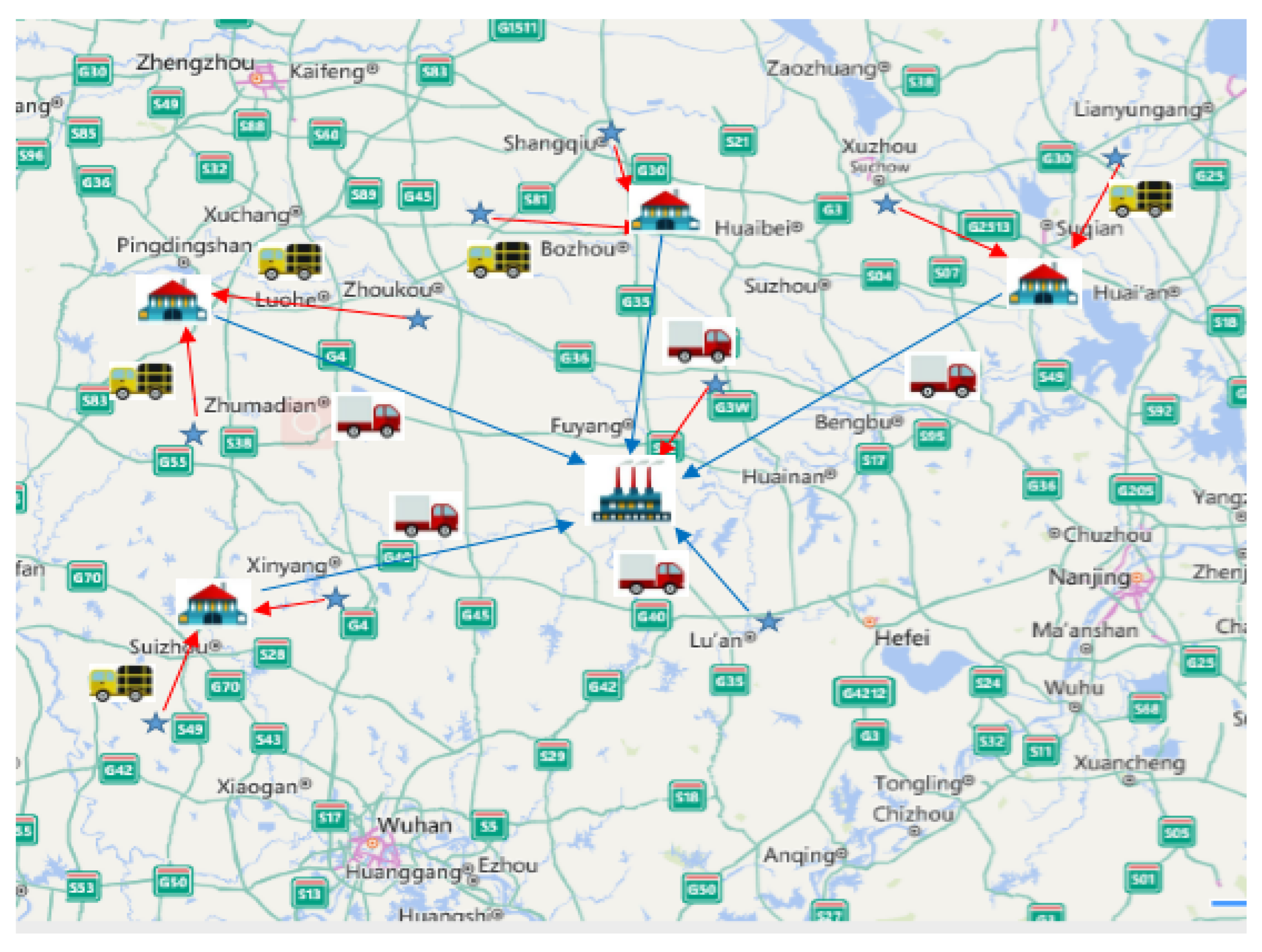
In order to explain the applicability of the model more clearly, a case of a bioethanol plant in central China is studied. The case considers both corn stover and wheat straw as the biomass raw materials, and adopts two baling techniques to transform the raw materials into rectangular bales and round bales, respectively. The corn stover, wheat straw, and other residues left after harvest can be used for bioethanol production all year round.

The biomass raw material acquisition of the bioethanol plant is shown in Figure 2. The recycling sites from different areas are established to distribute the biomass raw materials. First, biomass raw materials are packed into round or rectangular shapes for further production. Then, it will be collected uniformly by the recycling sites. In order to facilitate the recycling usage of the biomass raw materials, the recycling sites are generally built on the side of the road. The bioethanol plant procures the raw materials from suppliers according to production demand.

In this case, the biomass raw materials purchased by different suppliers may be packed in different ways. The two types of biomass raw materials with different packing shapes are transported to the bioethanol plant for processing. In the bioethanol plant, the biomass raw materials are firstly crushed into tiny particles and are then converted into saccharified liquid. Finally, the saccharified liquid is stored in the bioethanol fermentation tank for fermentation to produce bioethanol.

In the bioethanol plant, the storage cost of the biomass raw materials varies with the packing methods and the storage methods [26,37,38]. When the biomass raw materials are stored in the warehouse, they are covered with a tarpaulin and are placed on the ground, and thus would lead to a certain proportion of material loss, called storage loss. For convenience, the storage loss rate of the biomass raw materials is assumed to be constant [21,39,40]. Additionally, the material loss during the transportation is negligibly small. The basic parameter values are derived from the research paper as shown in

Table 5. Raw material prices and storage costs.

Parameter	Value
Unit storage cost of ethanol (USD/L)	$CE=0.65$
Unit storage cost of pelleted wheat straw (USD/ton)	$C{W}_{33t}=1.15$
Unit storage cost of round wheat straw (USD/ton)	$C{W}_{23t}=17.78$
Unit storage cost of rectangular wheat straw (USD/ton)	$C{W}_{13t}=10.75$
Unit storage cost of pelleted corn stover (USD/ton)	$C{W}_{32t}=0.08$
Unit storage cost of round corn stover (USD/ton)	$C{W}_{21t}=C{W}_{22t}=0.84$
Unit storage cost of rectangular corn stover (USD/ton)	$C{W}_{11t}=C{W}_{12t}=4.84$
The price of granulated wheat straw (USD/ton)	$P{M}_{13}=38$
The price of round wheat straw (USD/ton)	$P{M}_{12}=49.88$
The price of rectangular wheat straw (USD/ton)	$P{M}_{11}=41.63$
The price of granulated corn stalks (USD/ton)	$P{M}_{23}=32.3$
The price of round corn stalks (USD/ton)	$P{M}_{22}=80$
The price of rectangular corn stalks (USD/ton)	$P{M}_{21}=70$

,

Table 6. Dry matter loss and transportation costs.

Parameter	Value
Loss rate of rectangular raw materials at the bioethanol plant	${\theta }_{11}={\theta }_{21}=0.40$
Loss rate of round raw materials at the bioethanol plant	${\theta }_{12}={\theta }_{22}=0.17$
Loss rate of pelleted raw materials at the bioethanol plant	${\theta }_{13}={\theta }_{23}=0.32$
Loss rate of intermediate goods warehouse	${\vartheta }_i=0.09$
Unit cost of transporting rectangular raw materials (USD/ton/km)	$C{T}_{11}=C{T}_{21}=0.24$
Unit cost of transporting round raw materials (USD/ton/km)	$C{T}_{12}=C{T}_{22}=0.32$
Unit cost of transporting pelleted raw materials (USD/ton/km)	$C{T}_{13}=C{T}_{23}=0.09$

and

Table 7. Bioethanol productivity and storage capacity.

Parameter	Value
Conversion rate from corn stalk to bioethanol	${\gamma }_{11}=335$,${\gamma }_{12}=335$
Conversion rate from wheat straw to bioethanol	${\gamma }_{21}=310$,${\gamma }_{22}=310$
Bioethanol plant capacity (L/day)	$P=17000$
Cost of ethanol fermentation (USD/ton)	$CE=70$
Bioethanol plant raw material storage capacity (ton)	$S=1000$
Bioethanol storage capacity of bioethanol plant (L)	$C=20000$
Minimum stock in warehouse (ton)	$W_{bkt}=100$

[41,42].

5.2. Result

Based on the basic case parameters listed in Table 5, Table 6 and Table 7, the sensitivity of selected parameters was investigated. The model was solved using LINGO 11.0 on a personal computer. The processor was Intel Core i5-4200M 2.50 GHz.

The proposed dual-objective optimization model was solved using the solution method in Section 4.3. To analyze the dual membership functions, Figure 3 presents the curve of the membership $F_1$ and $F_2$ varying with $W_1$. When $W_1=0$, the value of $F_1$ is 0.4757715, $F_2$ is 1. At this time, it means that the constraint of carbon emission is more weighted than that of the economic goal, and carbon emission is at the minimum. Additionally, when $W_1=1$, the value of $F_1$ is 1, $F_2$ is 0.2032792. It means that the economic objective has the highest weight, while the carbon emission objective function has the lowest weight. As can be seen from Figure 3, $F_1$ increases by 82.77%, when $W_1=0.4$. As the importance of controlling carbon emissions decreases, $F_2$ becomes very small. Especially, when $W_1\ge 0.7$, the value of $F_2$ declines dramatically. Therefore, the value of $W_1\in [0.4,0.7]$ is preferred to take into account the membership of $F_1$ and $F_2$ simultaneously. As shown in Figure 4, when $W_1$ is between [0, 0.3], carbon emissions and total profits remain basically unchanged. When $W_1=0.4$, the total profit increases by 23.91% as carbon emissions increase. However, when $W_1$ is greater than 0.7, the total profit starts to decrease with the increase of carbon emissions and reaches the maximum value at $W_1=0.7$. Without loss of generality, the weight combination of $W_1=0.7$ and $W_2=0.3$ is chosen as a satisfactory scenario to further analyze the solution results.

5.2.1. Ethanol Production

According to the parameters listed in Table 4, Table 5 and Table 6, the optimal cost of raw material procurement, pretreatment, ethanol production, storage, carbon dioxide treatment, and transportation can be obtained, and are presented in Figure 5. In the conventional case, the cost of procuring biomass raw materials accounts for the largest proportion reaching 45.57% of the overall cost, followed by pretreatment of 31.93%. The following two are the cost of ethanol production and storage, which are 15.74% and 5.34%, respectively. Transportation and carbon emission treatment have the least impact on the total cost.

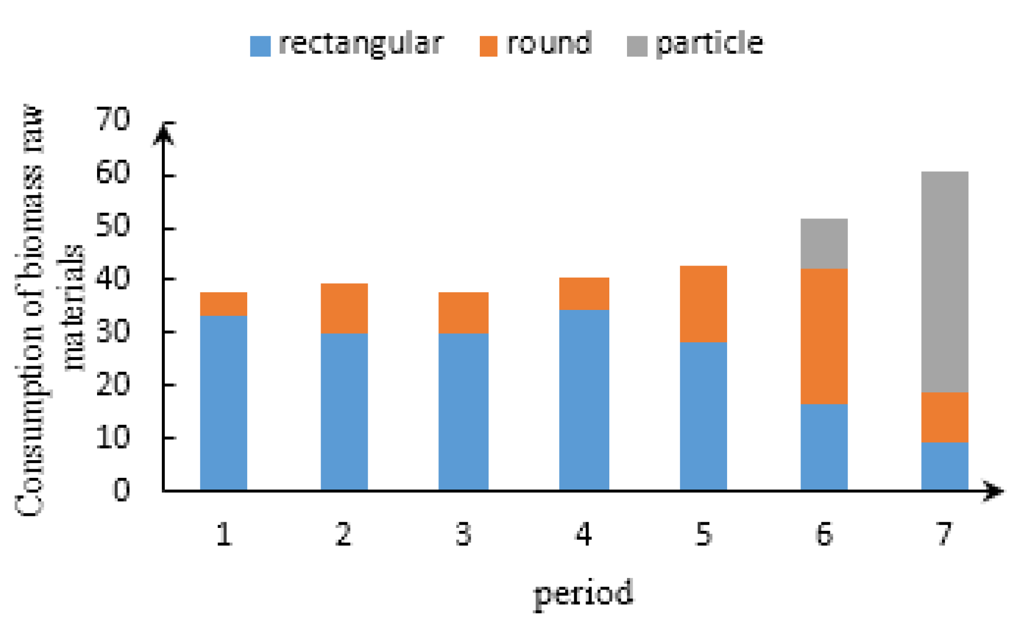
Figure 6 shows the raw materials of wheat straw and corn stover biomass processed by the bioethanol plant at various periods. Bioethanol plants treat corn stalks when they are available, and only select wheat stalks when corn stalks are insufficient. Figure 7 summarizes the amount of raw materials processed by the bioethanol plant in each period. In addition, the price of granulated biomass raw materials is slightly higher than the other two packaging methods, resulting in the bioethanol plant being unable to use the third way of packaging the biomass raw materials.

5.2.2. Carbon Emission and Total Profit

In order to analyze the relationship between carbon emission and total profit under the dual-objective optimization scheme, the following three optimization schemes are proposed to optimize the model. In scenario 1, the total profit is taken as the optimization target without considering the impact of carbon emissions. In scenario 2, the minimum solution of the carbon emission target is taken as the constraint condition and is substituted into the subobjective function of the carbon emission treatment to obtain the maximum total profit. In scenario 3, both the constraint of carbon emission and the constraint of total profit are considered, so as to obtain higher economic benefits under the condition of low carbon emission level. The optimal solution of carbon emission target and total economic cost under three scenarios is shown in

Table 8. Optimal target results in different scenarios.

	Carbon Emissions (kgCO2)	Total Profit (USD)
Scenario 1	10,555	51,981
Scenario 2	7657	28,571
Scenario 3	8200	49,790

. In scenario 2, carbon emissions are minimal, but the total profit is minimal due to stringent carbon measures. In scenario 1, there are no restrictions on carbon emissions, resulting in the highest carbon emissions.

To quantify the importance of the two objectives, the curve of carbon emission and total profit is drawn under different weight combinations of $W_1$ and $W_2$. As shown in Figure 4, both the total profit and carbon emission increase as $W_1$ increases. When $W_1=0.4$, the total profit increases dramatically by 23.91%. Meanwhile, as $W_1$ continues to increase, total profits level off. The carbon emission shows rapid growth when $W_1\ge 0.7$, while the total profit does not change much as the carbon emission continues to increase.

When $W_1=0.7$, the objective function obtains the optimal solution, and the quantity of raw materials delivered to the factory for pretreatment in each period of the bioethanol factory is shown in

Table 9. The number of raw materials delivered to the factory for pretreatment in each period.

Periods	1	2	3	4	5	6	7
Corn stover (ton)	32.81	36.57	57.05	27.59	31.57	32.57	29.57
Wheat straw (ton)	30.57	19.12	12.5	16.2	19.41	49.36	60.91

. At the same time,

Table 10. The quantity of raw materials delivered to the factory to manufacture ethanol in each period.

Periods	1	2	3	4	5	6	7
Corn stover (ton)	32.13	36.13	30.58	29.65	22.39	0	0
Wheat straw (ton)	30.13	18.67	12.06	15.76	19.21	29.2	0

shows the number of biomass raw materials transported to the factory for ethanol production in each period.

5.2.3. Sensitive Analysis

In this subsection, the sensitivity of the independent parameters is analyzed, and the impact of the choice of preprocessing on the relevant decision is discussed. By analyzing the sensitivity of individual parameters, decision-makers can help to determine the effect of parameter changes on the overall optimization.

The article establishes three scenarios for sensitivity analysis. Scenario 1 considers the impact of demand on the production plan, keeping other conditions unchanged, changing the market’s demand for bioethanol (increase/decrease), analyzing the impact of changing the demand for bioethanol on the objective function. Scenario 2 under the condition that other conditions remain unchanged, the factory production pretreatment cost is changed, and the impact of reducing production cost on the production plan is analyzed. Scenario 3 considers carbon emission factors, and discusses the impact of carbon emission factors on the objective function by analyzing the changes in carbon emission in each production link.

The production scheduling scheme and the cost of each part of the bioethanol plant under the given conditions are calculated. Then we consider the changes of the cost and carbon emission as the demand increases or decreases by 10%. As shown in

Table 11. Sensitive analysis as demand changes.

	10% Increase in Demand	10% Decrease in Demand
Total profit (USD)	51,353	46,224
Pretreatment (USD)	17,514	16,082
Warehouse storage (USD)	2795	3031
Mixed pretreatment (ton)	12.54	3.36
Ethanol production (USD)	8641	7916
Carbon emission (kgCO2)	8287	8002

, total profit increases by 3.13% when demand increases by 10%. At this time, 12.54 tons of biomass raw materials are treated by mixed pretreatment methods. The volume of carbon emission has also increased by 1.06% as demand increases. However, when demand falls down, the total profit decreases by 7.16%. There are fewer raw materials treated by the mixed pretreatment methods.

The second scenario analyzes the impact of pretreatment costs. The cost of pretreatment directly influences the selection of a proper pretreatment method. Similarly, a reduction and an increase by 10% of the pretreatment price is conducted to observe the changes of each part of the objectives. As shown in

Table 12. Sensitivity analysis as the pretreatment cost changes.

	10% Increase in Pretreatment Cost	10% Decrease in Pretreatment Cost
Total profit (USD)	45,535	51,918
Pretreatment (USD)	21,333	14,950
Warehouse storage (USD)	2859	2859
Mixed pretreatment (ton)	10.24	12.36
Ethanol production (USD)	8419	8419
Carbon emission (kgCO2)	8200	8200

, when the price of pretreatment mode decreases by 10%, the total profit increases by 4.27%. With the increase of total profit, more biomass raw materials are pretreated by the mixed pretreatment method, and are increased by 20.7%. Due to the carbon limits, the total emission quantity remains unchanged.

The third scenario analyzes the impact of carbon emissions on the dual-objective optimization model. There are three scenarios for analyzing carbon emission. In scenario 1, the unit treatment cost of carbon emission is the base value. In scenario 2, the unit processing cost of carbon emission is reduced by 10% from the base value. In scenario 3, the unit processing cost of carbon emission increases by 10% over the base value. As shown in

Table 13. The value of each link of bioethanol plant changing with the carbon emissions.

	Scenario 1	Scenario 2	Scenario 3
Total profit (USD)	49,790	50,218	49,503
Pretreatment (USD)	17,078	16,942	17,106
Warehouse storage (USD)	2859	2859	2859
Mixed pretreatment (ton)	3.36	3.36	3.36
Ethanol production (USD)	8419	8419	8419
Carbon emissions (kgCO2)	8200	8549	7873

, when the unit treatment cost of carbon emission decreases, the total profit increases. When the carbon emission increases by 4.2%, the total profit increases by 0.86%. Since the increase in carbon emission has no effect on product demand, the inventory and the amount of ethanol produced remain unchanged.

6. Conclusions

This work studied the production planning and scheduling problems of biofuel plants by comprehensively considering the impact of carbon emissions in each link of the production process. A MILP model with dual optimization objectives was established to quantify the trade-off between the total profit and carbon emission. The model was further solved by a dual-objective optimization approach to achieve Pareto solutions of the above two scalable goals with different numerical equivalent.

However, the sensitivity analysis showed that the mixed pretreatment method is beneficial as long as there is reduction on the pretreatment cost and a modest change of the demand for bioethanol. In a unit period, the total profit rose by 4.27% when the cost of pretreatment dropped by 10%. When the pretreatment cost is too high, the factory will give priority to using raw materials with a higher ethanol conversion rate for production. With the continuous development of ethanol production technology, when the cost falls to a suitable level, the pretreatment of the biomass raw materials will have a great impact on the total profit. Additionally, in the case of constant demand, the consumption of raw materials increased by 2% when the cost of pretreatment was reduced by 10%. At the same time, when the carbon emission policy is tightened, the bioethanol plant is faced with greater cost pressure.

There are some possible research directions for future work. The types of biofuel raw materials are diversified, and the additional products are also different. Therefore, it is worth considering the issue of plant production planning under comprehensive consideration of multiple biofuels and additional products. In addition, due to the large-scale problems in the production of biofuels, suitable heuristic algorithms should be used to solve the problems. Finally, in the face of demand, price and other parameter uncertainties, robust optimization, stochastic programming, and other methods can be used for in-depth research.