Fault Detection and Isolation System Based on Structural Analysis of an Industrial Seawater Reverse Osmosis Desalination Plant

Abstract

Currently, the use of industrial seawater reverse osmosis desalination (ISROD) plants has increased in popularity in light of the growing global demand for freshwater. In ISROD plants, any fault in the components of their control systems can lead to a plant malfunction, and this condition can originate safety risks, energy waste, as well as affect the quality of freshwater. This paper addresses the design of a fault detection and isolation (FDI) system based on a structural analysis approach for an ISROD plant located in Lima (Peru). Structural analysis allows obtaining a plant model, which is useful to generate diagnostic tests. Here, diagnostic tests via fault-driven minimal structurally overdetermined (FMSO) sets are computed, and then, binary integer linear programming (BILP) is used to select the FMSO sets that guarantee isolation. Simulations shows that all the faults of interest (sensors and actuators faults) are detected and isolated according to the proposed design.

1. Introduction

Currently, to satisfy the growing global demand for freshwater, seawater desalination technologies are being widely applied due the significant reduction in desalination cost, as well as the technological improvements incorporated within the desalination process [1,2]. These technologies have increased the security of water supplies for millions of people, and thus, seawater has become the only consistent available water source to cope with the growing shortage of freshwater [3,4]. Consequently, the seawater desalination industry has emerged as a vital sector to meet the demand of freshwater in different regions of the globe [5,6]. This industry will play a progressively vital role in guaranteeing the worldwide water supply [7].

Basically, desalination is any process that separates salt water into two flows: one with a low concentration of dissolved solids and other minerals and the other containing the remaining dissolved solids and minerals (concentrated or brine flow) [8]. Two basic commercially available technologies have been widely used for seawater desalination: thermal evaporation and membrane separation [5].

In the last few years, membrane based separation technology has dominated the market, and consequently, the reverse osmosis (RO) membrane separation technique has been increasingly implemented in industrial seawater desalination plants due to its better performance in terms of less energy consumption, higher water recovery rate, and low operational costs [9].

The advances obtained in the last 20 years in RO technology have allowed a reduction of up to 80% in the energy required for the production of desalinated water compared to other technologies, for example multi-stage flash (MSF) [10]. The RO process is more energy efficient than the MSF process because it operates at ambient temperature and there is no phase change requirement for salts’ removal [11]. Therefore, RO desalination plants are becoming predominant and extensively used worldwide [12].

In the RO process, the desalinated water flow obtained is called the permeate or product water, whereas the stream with concentrated salts is named the brine or reject [5].

Control systems are a vital component for the process industry [13,14], and therefore also for industrial seawater RO desalination plants because they ensure optimal operating conditions, quality desalted water, and personnel safety, as well as increasing the lifetime of the plants and reducing the desalination unit costs [15,16]. These control systems involve a great amount of unit processes, actuators, sensors, and controllers that are essential for the successful accomplishment of control strategies [17]. These components run under conditions of high pressure, variable frequency, and membrane fouling or scaling, which have an unwanted cost on the performance of these plants [18]. Therefore, all these components are susceptible to faults [19]. A fault is a violation of some specific normal behavior, which can lead to poor performance or the loss of plant functions. These faults can originate safety risks for plant personnel, physical damages, energy waste, as well as lead to poor freshwater quality, making it dangerous for human consumption [20]. These safety problems support the design of fault diagnosis and isolation (FDI) systems capable of detecting possible failures and making effective decisions to impede the dissemination of their effects and to maintain the safe operation of the industrial seawater reverse osmosis desalination (ISROD) plants [21].

In FDI systems, fault detection decides whether a fault has occurred and fault isolation finds in which component a fault has occurred [19]. The design of FDI systems for ISROD plants is crucial because a successful faults diagnosis can have major economic, social, and safety impacts [21,22,23]. In the last few years, some efforts have been carried out in order to develop FDI systems and fault tolerant control (FTC) for ISROD plants, commonly based on the use of statistical techniques and data-driven approaches; see, e.g., [22,23,24,25]. However, the design of these systems is a very complex task since the ISROD plants are characterized by having a large amount of interconnected sub-processes and instruments, with coupled variables between them [21].

Recently, structural analysis has been proposed as a potent method for designing FDI systems for complex industrial plants [26,27,28]. Structural analysis is an essential model based diagnosis method that uses graphic tools to competently assess fault detectability and the isolability of industrial plants without the accurate knowledge of plant parameters, and it can also be applied quantitatively to generate residuals for detecting and isolating faults [29].

In order to detect a fault and isolate the faulty component, an important task is to design diagnostic tests. In this paper, the use of structural analysis is proposed for the application of the novel concept of fault-driven minimal structurally overdetermined (FMSO) sets [28] to calculate efficient diagnostic tests, that is tests that have minimal structural redundancy and that are focused on a set of faults of interest.

The major contribution of this paper is the extension of the structural analysis approach to handle the case of the design of FDI systems for ISROD plants. In this way, in order to improve the FDI properties of the proposed system, diagnostic tests are obtained via FMSO sets. Furthermore, the binary integer linear programming (BILP) method, proposed in [27], is used for selecting FMSO sets to guarantee the maximum possible isolation.

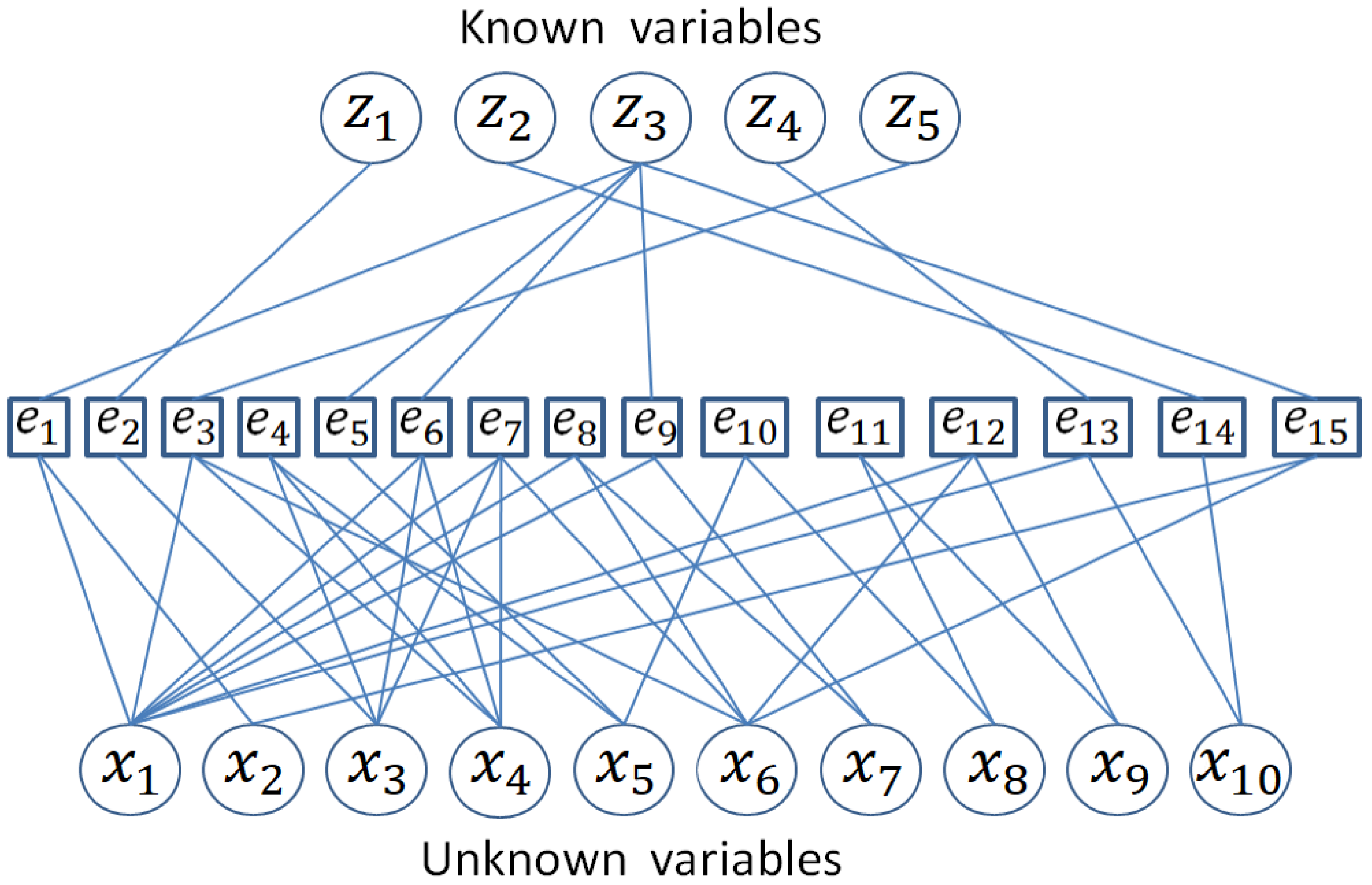
2. Structural Analysis for Model Based Diagnosis

Structural analysis is a useful tool for the design of model based fault diagnosis systems because it allows analyzing the properties of a system using graph theory [19]. Structural models can be represented by bipartite graphs. A graph is bipartite if its set of vertices can be separated into two disjoint sets $\mathsf{\Sigma }$ and X such that each edge has a connection in $\mathsf{\Sigma }$ and another in X.

The main assumption is that each component can be represented by a structural model composed of one or more equations; therefore, the variation of the behavior of at least one equation means that that component of the system is in a state of fault.

Definition 1 (System).

A system $\mathsf{\Sigma }(z,x,f)$ is a set of $n_e$ equations relating z known variables, x unknown variables, and $f$ faults.

The equations $e_k(z,x)\subseteq \mathsf{\Sigma }(z,x,f)$, $k=1,\cdots ,n_e$, can be differential or algebraic in z and x.

Definition 2 (Structural model).

The structural model of the system $\mathsf{\Sigma }(z,x,f)$ is a bipartite graph $G(\mathsf{\Sigma }\cup X\cup Z,A)$, or equivalently $G(\mathsf{\Sigma }\cup X,\mathcal{A})$, where $\mathcal{A}\subseteq A$ and $\mathcal{A}$ is a set of edges such that $a(i,j)\in \mathcal{A}$ iff variable $x_i$ is involved in equation $e_j$ [28].

To show these concepts, an academic model $\mathsf{\Sigma }$ is presented. $\mathsf{\Sigma }=\{e_1,e_2,\dots ,e_{15}\}$, and these fifteen equations relate $x=\{x_1,x_2,\dots x_{10}\}$ unknown variables and $z=\{z_1,z_2,\dots ,z_5\}$ known variables. The representation in a bipartite graph for this system is shown in Figure 1.

A key tool for fault diagnosis using structural analysis is the concept of matching. A matching is a causal assignment that links an equation with an unknown variable, where this equation can be used to calculate this unknown variable [19].

Definition 3 (Matching).

A matching $\mathcal{M}$ between Σ and X is a subset of A of disjoint edges of a bipartite graph G. It is called complete matching with respect to Σ or X if $\left|\mathcal{M}\right|=\left|\mathsf{\Sigma }\right|$ or $\left|\mathcal{M}\right|=\left|X\right|$ remains, respectively.

It is possible to find different matching for a specific bipartite graph; in Figure 2, a complete matching with respect to X (in bold edges) of the model $\mathsf{\Sigma }$ is shown.

Dulmage–Mendelsohn (DM) decomposition provides important structural properties, in particular for bipartite graphs. Each graph $G(\mathsf{\Sigma }\cup X,\mathcal{A})$ can be decomposed into three subgraphs [19]:

• Overdetermined subgraph $G^{+}$, with a X-complete matching that is not $\mathsf{\Sigma }$-complete,
• Just-determined subgraph $G^0$, with a complete matching,
• Underdetermined subgraph $G^{-}$, with a $\mathsf{\Sigma }$-complete matching that is not X-complete.

As a consequence of this bipartite graph decomposition, the corresponding system $\mathsf{\Sigma }$ can be decomposed into: ${\mathsf{\Sigma }}^{+}$ (overdetermined part), ${\mathsf{\Sigma }}^0$ (just-determined part), and ${\mathsf{\Sigma }}^{-}$ (underdetermined part).

Definition 4 (Structural redundancy).

Given a bipartite graph, the structural redundancy ${\rho }_{{}_{{\mathsf{\Sigma }}^{\prime }}}$ of a set of equations ${\mathsf{\Sigma }}^{\prime }\subseteq \mathsf{\Sigma }$ is defined as the difference between the number of equations and the number of unknown variables X [26].

The incidence matrix $\mathcal{I}$($e_i$,$x_j$) of the bipartite graph is used to represent this graph as a set $\mathcal{A}$ of edges in an algebraic manner. The rows of $\mathcal{I}$($e_i$,$x_j$) are the set of equations $e_i$, and the columns are the set of the variables $x_j$ with $i=1,\dots ,m$ equations and $j=1,\dots ,n_j$ variables. The edge ($e_i$,$x_j$) ∈$\mathcal{A}$ is associated with a “1” in the intersection of row $e_i$ and column $x_j$.

Structural Diagnosability

Analytical redundancy relations (ARRs) can be calculated when there are equations that are not necessary to match unknown variables in a system $\mathsf{\Sigma }$. Any overdetermined subgraph $G^{+}$ contains more equations than variables, and such an equation can be used for residual generation. A residual, derived from ARRs, is generated from a subgraph $G^{+}$ using the excess equations once all unknown variables within $G^{+}$ are expressed in terms of known variables. When an expected value of an $ARR$ is not met, a fault is detected.

Definition 5 (ARR).

An ARR is a constraint calculated from the system $\mathsf{\Sigma }(z,x,f)$ that contains only measured variables and can therefore be used for residual generation. ARRs can be obtained from $\mathsf{\Sigma }(z,x,f)$ by eliminating the unknown variables.

Definition 6 (Residual generator).

A residual generator creates residuals by using the model $\mathsf{\Sigma }(z,x,f)$ and the known variables z. A residual is a signal that is zero when the system is fault free, and not zero when faults are present.

A minimal structurally overdetermined set (MSO set) can be used to generate an $ARR$ given that the equation number exceeds the unknown variable number by one (structural redundancy of one), which means that only one residual generator can be developed. According to [27], the computation of MSO sets can be exponential according to the structural redundancy and system measurements. One way to reduce this computational cost can be by calculating only the MSO sets of interest, that is reducing the calculation only to those impacted by faults. Hence, the concept of the fault-driven minimal structurally overdetermined (FMSO) set is useful.

Let the FMSO set $\phi$, where $Z_{\phi }\subseteq Z$ is the set of known variables of $\phi$, $X_{\phi }\subseteq X$ is the set of unknown variables of $\phi$, and $F_{\phi }\subseteq F$ is the set of fault support of $\phi$, be defined as below.

Definition 7 (FMSO set).

A subset of equations $\phi \subseteq \mathsf{\Sigma }(z,x,f)$ is an FMSO set of $\mathsf{\Sigma }(z,x,f)$ if (1) $F_{\phi }\ne \varnothing$ and ${\rho }_{\phi }=1$, which means $\left|\phi \right|=|X_{\phi }|+1$, and (2) no proper subset of φ is overdetermined [28].

As an example, for the academic model in Figure 1, if a fault $f_1$ is included in Equation (1), using Definition 7, there are 53 FMSO sets. Figure 3 shows the bipartite graph of the first FMSO set ${\phi }_1=\{e_1,e_8,e_9,e_{13},e_{14},e_{15}\}$.

With this definition, given a fault $f\in F$, it is defined as a detectable fault if an FMSO set $\phi$ with $f\in F_{\phi }$ exists. Given two detectable faults $f_i$ and $f_j$ of $F(i\ne j)$, it is said that $f_i$ is isolable from $f_j$ if there exists a set $\phi$ such that $f_i\in F_{\phi }$ and $f_j\notin F_{\phi }$. Then, a group of FMSO sets can be properly chosen to detect and isolate each detectable and isolable fault, respectively. It is clear that not all faults in F are necessarily detectable or isolable.

The algorithm for the calculation of FMSO sets presented in [28], allows the calculation of all the FMSO sets related to the set of faults of interest, which can be many in the case of large and complex systems, and as a result, the fault detection and isolation (FDI) system can be designed.

3. Modeling of the Seawater RO Desalination Process

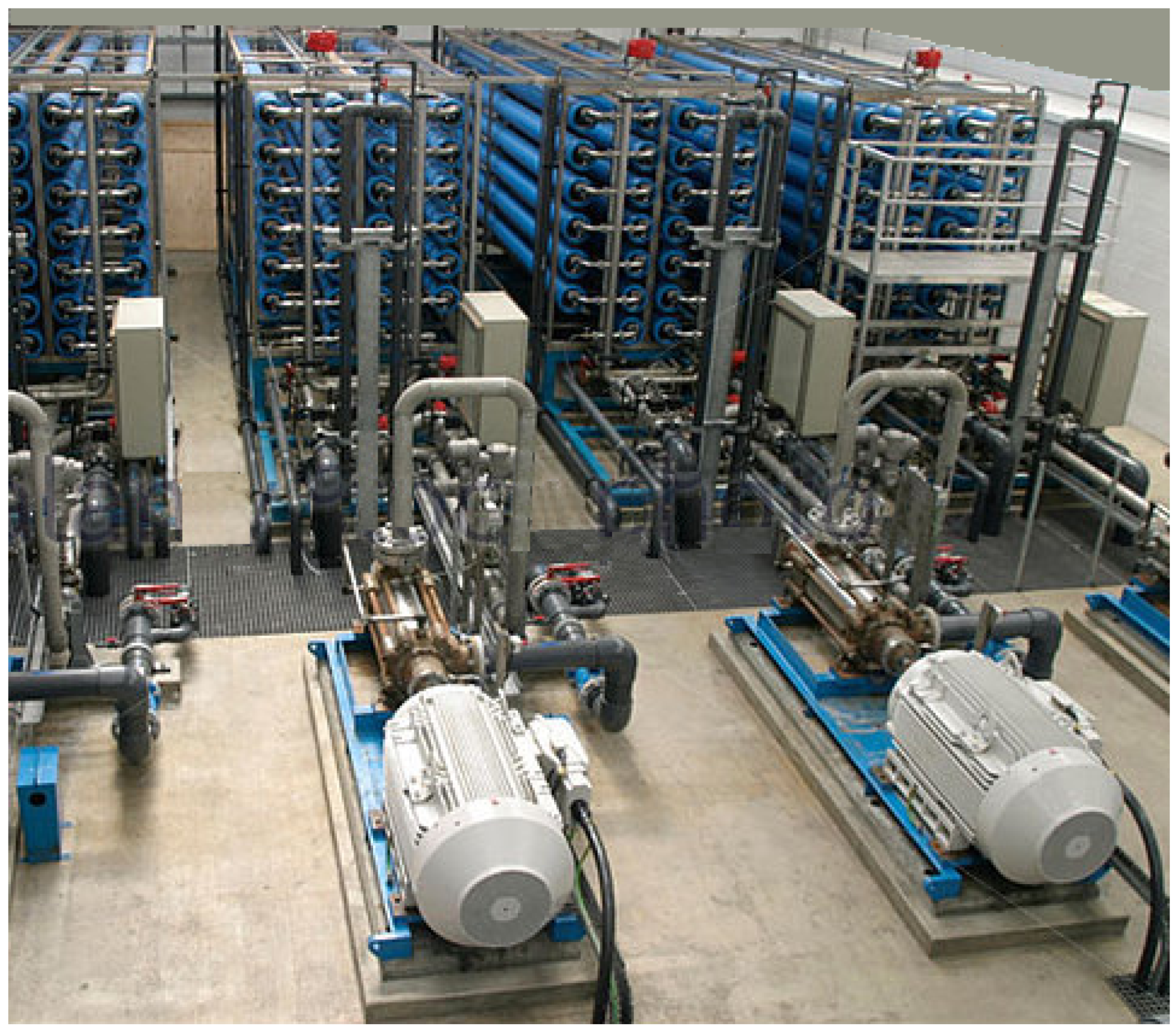
3.1. Brief Description of the Industrial Seawater RO Desalination Plant

The ISROD plant under study in this paper is located in Lima province (Peru), one of the extreme arid areas on the South American continent with an average annual rainfall of about 6.5 mm [30]. Therefore, the water supply to this region depends on the hydraulic resources from the catchments of the Chillón, Rímac, and Lurín rivers [30].

This plant has a freshwater production capacity in nominal operation of about 34,560 m³/day and provides new water supplies for industrial and domestic sectors. The technology applied in this plant is RO. The daily processed seawater volume by the plant is 76,800 m³; of this volume, 42,240 m³ of brine is sent back into the sea in a dispersive way. Thus, the conversion rate of the plant is 45%; this means that 45 L of guaranteed high quality freshwater are obtained from every 100 L of seawater.

The plant has the following subsystems: (1) seawater catchment, (2) pre-treatment, (3) RO, (4) post-treatment, (5) storage, and (6) brines management. The RO system is the most complex and the one that has the greatest importance in the production of quality fresh water [5]. Figure 4 shows a diagram of this industrial seawater RO desalination plant.

The pretreatment subsystem is made up of the following items: feed pumps, flocculation/sedimentation to eliminate suspended material, dissolved air flotation (DAF) to eliminate potential algal biomass or potential hydrocarbons, granular media filtration (GMF), low-pressure ultrafiltration (UF) or microfiltration (MF) to eliminate suspended particulate matter, and additives tanks. The resulting permeate stream undergoes a post-treatment procedure consisting of the addition of conditioning chemicals and residual disinfection. The obtained brine flow is carefully dispersed into the sea. This plant has four membrane RO racks with a production capacity per racks of 8640 m³/day. Each membranes rack consists of 140 pressure vessels, and each one has seven aromatic polyamide membranes. Figure 5 shows a view of the RO racks, and Figure 6 exhibits a schematic of one of the pressure vessels of these RO racks.

This plant is equipped with the following sensors and actuators: pH sensors, pressure sensors, temperature sensors, flow sensors, conductivity sensors, ultrasonic level sensors, additive dosing pumps, high-pressure feed pumps, and control valves. The nominal operation pressure of each RO membranes rack is 69 bar. The retentate valve is used to adjust the retentate flow and the membrane rack pressure.

Each RO membrane rack is controlled by a PAC (programmable automation controller). The plant has also a SCADA (Supervisory Control And Data Acquisition) that performs the supervision of the overall desalination plant.

3.2. Modeling of the Seawater RO Desalination Process

For the design of fault tolerant controllers, mathematical models that adequately describe the performance of the processes to be controlled are needed [19]. These models can differ in complexity according to the intended applications [20].

Different mathematical models for the solvent and solute transport through the RO membrane have been proposed by researchers; see, e.g., [31,32,33]. The most widely applied model is the one based on a solution-diffusion transport mechanism [34]. Figure 7 shows the diagram of the RO process used to obtain the model.

The mathematical modeling of the seawater RO desalination process presented in this section is based on first principles (mass, momentum, and energy balances), as well as on physical and chemical equations [22,27]. These equations have a set of parameters that need to fit in order to describe each specific RO process [22].

The osmotic pressure is represented by the equation [31]:

$$\begin{array}{c}\hfill \pi =R_{g}T\sum C_i\end{array}$$

(1)

where $\pi$ is the osmotic pressure, $R_g$ is the universal gas constant, T is the temperature, and $\sum C_i$ is the molar concentration of all constituents in a solution.

The overall fluid and solute (salt) mass balance equations are represented by [35]:

$$\begin{array}{c}\hfill Q_f=Q_p+Q_c\end{array}$$

(2)

$$\begin{array}{c}\hfill C_f{Q}_f=C_p{Q}_p+C_c{Q}_c\end{array}$$

(3)

where $Q_f$ is the feed stream, $Q_p$ is the permeate (solvent) stream, $Q_c$ is the brine (retentate) stream, $C_f$ is the salt concentration in the feed stream, $C_p$ is the salt concentration in the permeate stream, and $C_c$ is the salt concentration in the brine stream.

The diffusion of water across a semi-permeable RO membrane is described as [32]:

$$\begin{array}{c}\hfill J_w=A_w(\Delta P-\Delta \pi )\end{array}$$

(4)

where $J_w$ is the water (permeate) flux, $A_w$ is the water permeability coefficient, $\Delta P$ is the pressure difference between the high concentration side and low concentration side of the membrane, and $\Delta \pi$ is the osmotic pressure difference across the surface of the membrane.

The total permeate flow rate is obtained by:

$$\begin{array}{c}\hfill Q_p=A_m{n}_m{J}_w\end{array}$$

(5)

where $A_m$ is the area of each RO membrane and $n_m$ is the number of membranes.

The diffusion of salt across a semi-permeable RO membrane is attained as follows [32]:

$$\begin{array}{c}\hfill J_s=B(C_f-C_p)=C_p{J}_w\end{array}$$

(6)

where $J_s$ is the salt flux and B is the solute permeability constant.

The performance of the RO membranes is evaluated by the following parameters [33]: the salt rejection ratio ($SR$):

$$\begin{array}{c}\hfill SR=(1-\frac{C_p}{C_f})\ast 100\end{array}$$

(7)

and the recovery ratio ($R_r$):

$$\begin{array}{c}\hfill R_r=\frac{Q_p}{Q_f}\ast 100\end{array}$$

(8)

The permeate concentration is obtained from Equation (6) as:

$$\begin{array}{c}\hfill C_p=\frac{J_s}{J_w}=\frac{C_f}{1+\frac{A}{B}(\Delta P-\Delta \pi )}\end{array}$$

(9)

The permeate flow and the salt flow are obtained from Equations (2) and (8) as:

$$\begin{array}{c}\hfill Q_p=Q_f{R}_r\end{array}$$

(10)

$$\begin{array}{c}\hfill Q_c=Q_f(1-R_r)\end{array}$$

(11)

The evolution of the retentate stream velocity is obtained as [33]:

$$\begin{array}{c}\hfill \frac{\mathrm{d}{v}_r}{\mathrm{d}t}=\frac{A_p^2}{A_m{K}_{m}V}(v_f-v_r)+\frac{A_p}{\rho V}\Delta \pi -\frac{1}{2}\frac{A_p{e}_{vr}{v}_r^2}{V}\end{array}$$

(12)

where $v_r$ is the retentate stream velocity, $A_p$ is the pipe cross-sectional area, $K_m$ is the overall mass transfer coefficient, V is the system volume, $v_f$ is the feed stream velocity, $\rho$ is the fluid density, and $e_{vr}$ is the retentate valve resistance.

The permeate stream velocity ($v_p$) is attained as [34]:

$$\begin{array}{c}\hfill v_p=\frac{A_m{K}_m}{\rho A_p}(P_{sys}-\Delta \pi )\end{array}$$

(13)

where $P_{sys}$ is the system pressure, which is obtained as:

$$\begin{array}{c}\hfill P_{sys}=\frac{\rho A_p}{A_m{K}_m}(v_f-v_r)+\Delta \pi \end{array}$$

(14)

The concentration polarization equation based on the film theory at the feed side membrane is expressed as [34]:

$$\begin{array}{c}\hfill CP=\frac{C_m-C_p}{C_f-C_p}=exp\left(\frac{J_w}{K_m}\right)\end{array}$$

(15)

where $C_m$ is the salt concentration at the feed side membrane surface.

Equations (1)–(15) describe the steady-state performance of an RO process in a membrane module.

4. FDI System for the RO Desalination Plant under Study

As seen in Section 3, Equations (1)–(15) describe the steady-state performance of an RO process in a membrane module. To apply the structural analysis concepts presented in Section 2, it is necessary, first, to identify the known variables, the unknown variables, as well as the fault variables to be monitored and sum up the relations chosen for the FDI system design. The representation in a bipartite graph for this system is shown in Figure 8.

Applying Definition 1 to case study, the system $\mathsf{\Sigma }$ is composed of twenty equations, $e_1$ to $e_{20}$, relating to unknown variables $x=\{Q_f,Q_p,Q_c,C_f,C_p,C_c,v_f,v_p,v_r,J_w,\Delta P,\Delta \pi ,J_s,P_{sys},C_m\}$, which are internal plant variables, and the known variables $z=\{y_{Q_f},y_{Q_p},y_{Q_c},y_{C_f},y_{C_p},y_{C_c},y_{v_f},y_{v_p},y_{v_r},\}$, which are sensors and actuators.

There are also 10 faults considered $f=\{f_1,f_2,f_3,f_4,f_5,f_6,f_7,f_8,f_9,f_{10}\}$, 9 faults associated with sensors and 1 fault associated with the main actuator (high-pressure pump).

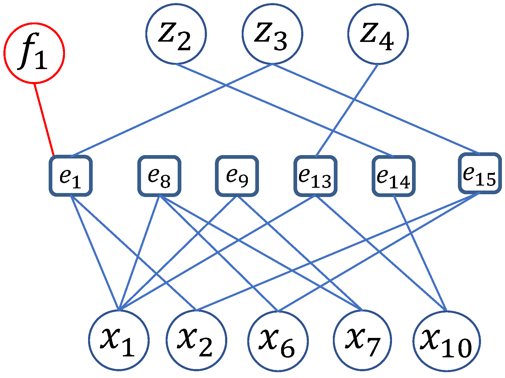
4.1. FMSO Sets’ Calculation

As presented in Section 2, computing MSO sets, it is possible to find analytical redundancy relations (ARR) with minimal structural redundancy, that is the equation number exceeds the unknown variable number by one. However, it cannot be guaranteed that these sets are related to any of the faults of the set of interest [36].

In this sense, FMSO sets are calculated using Definition 7 and its calculation algorithm. With this, a total of 19 FMSO sets can be found following the search algorithm presented in [28].

These FMSO sets are shown in

Table 1. FMSO sets found.

FMSO Set	Equations Involved
${\phi }_1$	$\{e_7,e_8,e_9,e_{10},e_{18},e_{19},e_{20}\}$
${\phi }_2$	$\{e_4,e_6,e_{13},e_{15},e_{16}\}$
${\phi }_3$	$\{e_2,e_{12},e_{13},e_{14},e_{15},e_{16},e_{17}\}$
${\phi }_4$	$\{e_2,e_4,e_6,e_{12},e_{14},e_{15},e_{16},e_{17}\}$
${\phi }_5$	$\{e_2,e_4,e_6,e_{12},e_{13},e_{14},e_{16},e_{17}\}$
${\phi }_6$	$\{e_2,e_4,e_6,e_{12},e_{13},e_{14},e_{15},e_{17}\}$
${\phi }_7$	$\{e_1,e_{12},e_{13},e_{14}\}$
${\phi }_8$	$\{e_1,e_4,e_6,e_{12},e_{14},e_{15},e_{16}\}$
${\phi }_9$	$\{e_1,e_2,e_{13},e_{14},e_{15},e_{16},e_{17}\}$
${\phi }_{10}$	$\{e_1,e_2,e_{12},e_{14},e_{15},e_{16},e_{17}\}$
${\phi }_{11}$	$\{e_1,e_2,e_{12},e_{13},e_{15},e_{16},e_{17}\}$
${\phi }_{12}$	$\{e_1,e_2,e_4,e_6,e_{14},e_{15},e_{16},e_{17}\}$
${\phi }_{13}$	$\{e_1,e_2,e_4,e_6,e_{13},e_{14},e_{16},e_{17}\}$
${\phi }_{14}$	$\{e_1,e_2,e_4,e_6,e_{13},e_{14},e_{15},e_{17}\}$
${\phi }_{15}$	$\{e_1,e_2,e_4,e_6,e_{12},e_{15},e_{16},e_{17}\}$
${\phi }_{16}$	$\{e_1,e_2,e_4,e_6,e_{12},e_{14},e_{16},e_{17}\}$
${\phi }_{17}$	$\{e_1,e_2,e_4,e_6,e_{12},e_{14},e_{15},e_{17}\}$
${\phi }_{18}$	$\{e_1,e_2,e_4,e_6,e_{12},e_{13},e_{16},e_{17}\}$
${\phi }_{19}$	$\{e_1,e_2,e_4,e_6,e_{12},e_{13},e_{15},e_{17}\}$

.

4.2. Fault Detection and Isolation

By definition, it can be stated that a fault f is detectable if there is an FMSO set $\phi$ whose set of faults $F_{\phi }$ includes the fault under study $f\in F_{\phi }$.

Besides, as mentioned in Section 2, given two different detectable faults $f_i$ and $f_j$, it is said that $f_i$ is isolable from $f_j$ if there exists a set $\phi$ such that $f_i\in F_{\phi }$ and $f_j\notin F_{\phi }$.

By applying these concepts to the fault signatures of all the FMSO sets found for the process under study, it is determined that each of the faults in the set of faults of interest belongs to one of the FMSO sets found, so it can be stated that all faults are detectable. However, not all faults can be isolated with the available known variables. To complete the design of the FDI system and select the FMSO sets, three faults that are not isolatable between them are grouped together in a mixed fault.

Faults that cannot be isolated from each other are displayed in Figure 9. It can be seen that from all 10 faults, seven are completely detectable and isolable, but three of them are not isolable from each other; these faults are considered as one mixed fault $\{f_7,f_8,f_9\}$.

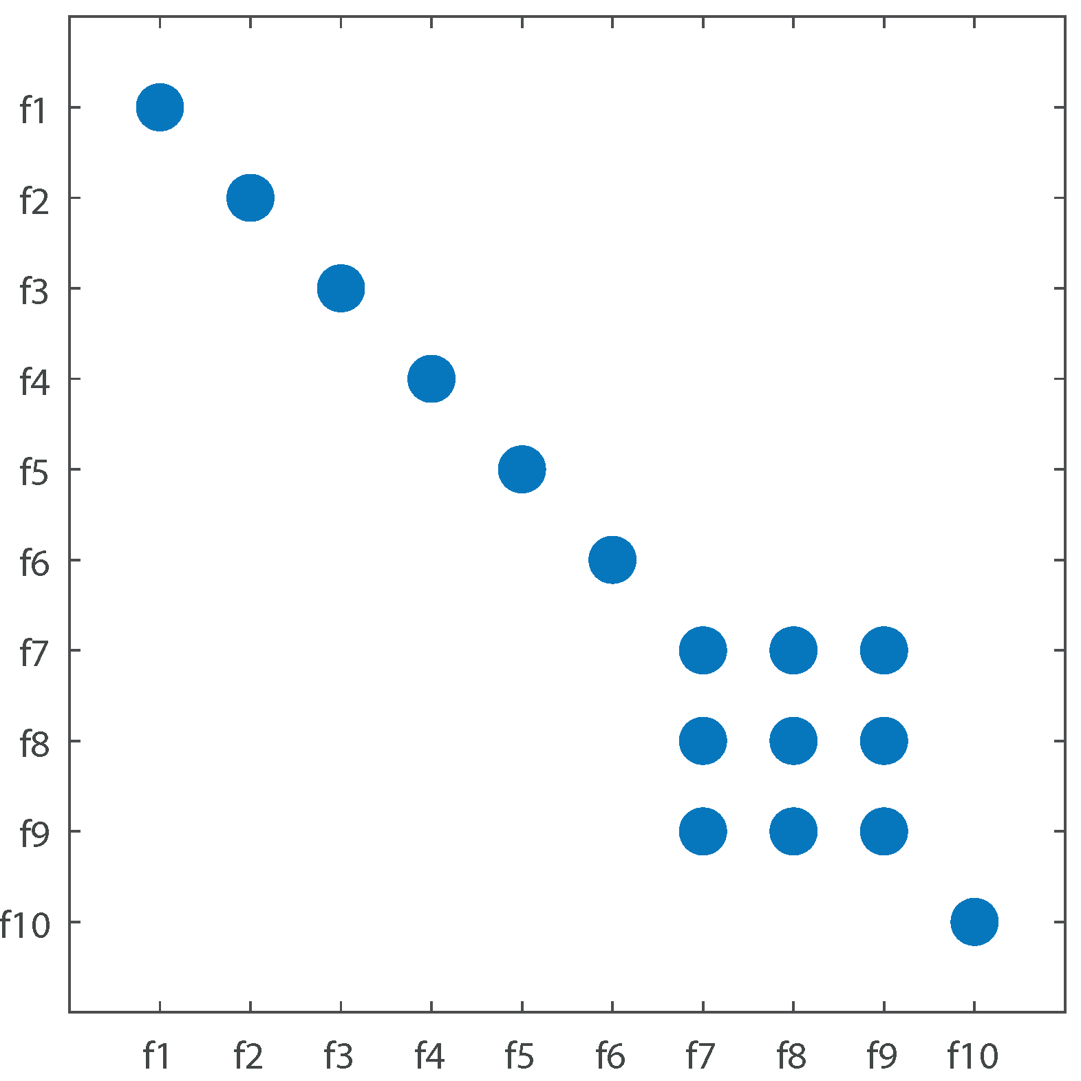
4.3. FMSO Sets’ Selection by the BILP Method

Given the set of local FMSO sets calculated for the RO desalination plant, the BILP method, proposed in [27], is used for selecting FMSO sets to guarantee the maximum possible isolation for subsystem $\mathsf{\Sigma }$. Applying this algorithm, a set of five FMSOs is selected for full detection and possible isolation of considered faults. The set of FMSO sets selected is shown in the following equation:

$$\begin{array}{c}\hfill \mathsf{\Phi }=\{{\phi }_1,{\phi }_6,{\phi }_7,{\phi }_9,{\phi }_{16}\}\end{array}$$

(16)

4.4. Residual Generation

Applying Definitions 5 and 6, all FMSO sets of Equation (16) are used to generate the five residual generators $arr$ of the FDI system designed; for each FMSO $\phi$, a complete matching ${\mathcal{M}}_{\phi }$ is selected; by definition, $\phi$ has exactly one equation out of the matching as its structural redundancy is one. In this way, the extra equation within $\phi$ is used as a residual generator $ar{r}_{\phi }$, and its expected value is null during nominal operation (fault free). The fault signature matrix of the FDI system designed is shown in

Table 2. Fault diagnosis system of the fault detection and isolation (FDI) system designed.

	${\mathit{f}}_1$	${\mathit{f}}_2$	${\mathit{f}}_3$	${\mathit{f}}_4$	${\mathit{f}}_5$	${\mathit{f}}_6$	${\mathit{f}}_7,{\mathit{f}}_8,{\mathit{f}}_9$	${\mathit{f}}_{10}$
$ar{r}_1$	0	0	0	0	0	0	1	0
$ar{r}_6$	1	1	1	1	0	1	0	0
$ar{r}_7$	1	1	1	0	0	0	0	1
$ar{r}_9$	0	1	1	1	1	1	0	1
$ar{r}_{16}$	1	0	1	0	1	1	0	1

.

5. Results and Discussion

The fault detection and isolation system for the four membrane RO racks was programmed in an industrial PAC controller that had the computational capacity to calculate the residual signals in real time from the signals of the known variables (sensors and actuators). See Figure 10.

For simulation purposes, each fault of the set of faults of interest was introduced during operation for a time interval (t = 500–800 s) to evaluate the FDI system performance. In Figure 11, the residuals selected $ar{r}_1$, $ar{r}_6$, $ar{r}_7$, $ar{r}_9$, and $ar{r}_{16}$ are shown in the presence of all faults considered.

According to Figure 11, it follows that faults $f_7$, $f_8$, and $f_9$ are detected and isolated together with $ar{r}_1$ directly because the corresponding equations that contain these faults ($e_{18},e_{19},e_{20}$) are contained only within the FMSO set ${\phi }_1$, as seen in Table 1, and the occurrence of any of these faults directly impacts only the residual $ar{r}_1$; therefore, they are detectable, but not isolable; these faults are related directly to sensors $y_{v_f},y_{v_p}$, and $y_{v_r}$. These sensors are used only for monitoring and fault diagnosis purposes; hence, with the occurrence of any of these faults, the control loop and therefore the operability of the plant are not critically compromised. However if it is required to isolate them individually, there are two possible solutions. One of them is hardware redundancy; this means adding sensors and consequently adding more known variables with which to calculate new FMSO sets to calculate extra residuals for isolation. The other solution is using software redundancy; this means designing observers whose observed variables are considered as known variables and, in this way, generating more FMSO sets to calculate extra residuals for isolation. For all other faults, a specific fault signature is required to detect and isolate them. For example, to detect fault $f_1$, the ARRs $ar{r}_7$ and $ar{r}_{16}$ are monitored; however, to isolate fault $f_1$ from fault $f_3$, which is also sensitive to ARRs $ar{r}_7$ and $ar{r}_{16}$, it is necessary to additionally check the ARRS $ar{r}_6$ and $ar{r}_9$; in the same way, to isolate fault $f_1$ from fault $f_{10}$, it is necessary to additionally monitor $ar{r}_9$.

Therefore, it was demonstrated that the designed FDI system based on structural analysis constitutes a useful tool to perform fault detection and isolation in industrial seawater RO desalination plants.

Finally, the FDI system designed was incorporated into the SCADA of the process that performs the supervision of the overall ISROD plant.

6. Conclusions

The design of a fault detection and isolation system based on structural analysis of an ISROD plant located in Lima (Peru) was developed. This FDI system is composed of five analytical redundancy relations obtained from five diagnostic tests. The latter were selected from a set of 19 candidate FMSO sets using the BILP method. The FDI system was tested by the simulation of the diagnostic tests obtained, validating that the 10 faults of the set of interest, which include 9 sensor faults and 1 actuator fault, can be detected. Our future work will focus on solving the problem of sensor placement in order to isolate the set of three faults that cannot be isolated from each other with the current ISROD plant instrumentation.

References

1. Gao, L.; Yoshikawa, S.; Iseri, Y.; Fujimori, S.; Kanae, S. An economic assessment of the global potential for seawater desalination to 2050. Water 2017, 9, 763. [Google Scholar] [CrossRef]
2. Ghaffour, N.; Missimer, T.M.; Amy, G.L. Technical review and evaluation of the economics of water desalination: Current and future challenges for better water supply sustainability. Desalination 2013, 309, 197–207. [Google Scholar] [CrossRef] [Green Version]
3. Rivas-Perez, R.; Sotomayor-Moriano, J.; Pérez-Zuñiga, G.; Soto-Angles, M.A. Real-time implementation of an expert model predictive controller in a pilot-scale reverse osmosis plant for brackish and seawater desalination. Appl. Sci. 2019, 9, 2932. [Google Scholar] [CrossRef] [Green Version]
4. Said, S.A.; Emtir, M.; Mujtaba, I.M. Flexible design and operation of multi-stage flash (MSF) desalination process subject to variable fouling and variable freshwater demand. Processes 2013, 1, 279–295. [Google Scholar] [CrossRef]
5. Voutchkov, N. Desalination Engineering: Planning and Design; McGraw Hill Professional: New York, NY, USA, 2011. [Google Scholar]
6. Rivas-Perez, R.; Sotomayor-Moriano, J.; Perez-Zuñiga, C.G. Adaptive expert generalized predictive multivariable control of seawater RO desalination plant for a mineral processing facility. IFAC-PapersOnLine 2017, 50, 10244–10249. [Google Scholar] [CrossRef]
7. Peñate, B.; García-Rodríguez, L. Current trends and future prospects in the design of seawater reverse osmosis desalination technology. Desalination 2012, 456, 136–149. [Google Scholar] [CrossRef]
8. Wang, L.K.; Chen, J.P.; Hung, Y.-T.; Shammas, N.K. Handbook of Environmental Engineering: Membrane and Desalination Technology; Humana Press: New York, NY, USA, 2011; Volume 13. [Google Scholar]
9. Qasim, M.; Badrelzaman, M.; Darwish, N.N.; Darwish, N.A.; Hilal, N. Reverse osmosis desalination: A state-of-the-art review. Desalination 2019, 459, 59–104. [Google Scholar] [CrossRef] [Green Version]
10. Kim, J.; Park, K.; Yang, D.R.; Hong, S. A comprehensive review of energy consumption of seawater reverse osmosis desalination plants. Appl. Energy 2019, 254, 113652. [Google Scholar] [CrossRef]
11. Park, K.; Jungbin, K.; Yang, D.R.; Hong, S. Towards a low-energy seawater reverse osmosis desalination plant: A review and theoretical analysis for future directions. J. Membr. Sci. 2020, 595, 117607. [Google Scholar] [CrossRef]
12. Greenlee, L.F.; Lawler, D.F.; Freeman, B.D.; Marrot, B.; Moulin, P. Reverse osmosis desalination: Water sources, technology, and today’s challenges. Water Res. 2009, 43, 2317–2348. [Google Scholar] [CrossRef]
13. Aström, K.; Hägglund, T. Control PID Avanzado; Pearson Educación, S.A.: Madrid, Spain, 2009. [Google Scholar]
14. Rodriguez Vazquez, J.R.; Rivas-Perez, R.; Sotomayor Moriano, J.J.; Peran Gonzalez, J.R. Advanced control system of the steam pressure in a fire-tube boiler. IFAC Proc. Vol. 2008, 41, 11028–11033. [Google Scholar] [CrossRef] [Green Version]
15. Alatiqi, I.; Ettourney, H.; El-Dessouky, H. Process control in water desalination industry: An overview. Desalination 1999, 126, 15–32. [Google Scholar] [CrossRef]
16. Feliu-Batlle, V.; Rivas-Perez, R.; Linares-Saez, A. Fractional order robust control of a reverse osmosis seawater desalination plant. IFAC-PapersOnLine 2017, 50, 14545–14550. [Google Scholar] [CrossRef]
17. Gambier, A.; Wellenreuther, A.; Badreddin, E. Control system design of reverse osmosis plants by using advanced optimization techniques. Desalin. Water Treat. 2009, 10, 200–209. [Google Scholar] [CrossRef] [Green Version]
18. Gambier, A.; Miksch, T.; Badreddin, E. Fault-tolerant control of a small reverse osmosis desalination plant with feed water bypass. In Proceedings of the 2010 American Control Conference, Baltimore, MD, USA, 30 June–2 July 2010; pp. 3611–3616. [Google Scholar]
19. Blanke, M.; Kinnaert, M.; Lunze, J.; Staroswiecki, M.; Schröder, J. Diagnosis and Fault Tolerant Control; Springer: Berlin/Heidelberg, Germany, 2003. [Google Scholar]
20. Vásquez, J.W.; Perez, C.G.; Muñoz, Y.A.; Ospino, A. Simultaneous occurrences and false-positives analysis in discrete event dynamic systems. J. Comput. Sci. 2020, 44, 101162. [Google Scholar] [CrossRef]
21. Achbi, M.S.; Kechida, S. Methodology for monitoring and diagnosing faults of hybrid dynamic systems: A case study on a desalination plant. Diagnostyka 2020, 21, 20–33. [Google Scholar]
22. Gambier, A.; Blümlein, N.; Badreddin, E. Real-time fault tolerant control of a reverse osmosis desalination plant based on a hybrid system approach. In Proceedings of the 2009 American Control Conference, St. Louis, MO, USA, 10–12 June 2009; pp. 1598–1603. [Google Scholar]
23. McFall, C.W.; Christofides, P.D.; Cohen, Y.; Davis, J.F. Fault tolerant control of a reverse osmosis desalination process. In Proceedings of the 8th International IFAC Symposium on Dynamics and Control of Process Systems, Cancun, Mexico, 4–6 June 2007; Volume 3, pp. 161–166. [Google Scholar]
24. Garcia-Alvarez, D.; Fuente, M.J. A UPCA based monitoring and fault detection approach for reverse osmosis desalination plants. Desalin. Water Treat. 2014, 52, 1272–1286. [Google Scholar] [CrossRef]
25. Pascual, X.; Gu, H.; Bartman, A.; Zhu, A.; Rahardianto, A.; Gira, J. Fault detection and isolation in a spiral-wound reverse osmosis (RO) desalination plant. Ind. Eng. Chem. Res. 2014, 53, 3257–3271. [Google Scholar] [CrossRef]
26. Pérez-Zuñiga, C.G.; Sotomayor-Moriano, J.; Chanthery, E.; Travé-Massuyès, L.; Soto, M. Flotation process fault diagnosis via structural analysis. IFAC-PapersOnLine 2019, 52, 225–230. [Google Scholar] [CrossRef]
27. Pérez-Zuñiga, C.G.; Chanthery, E.; Travé-Massuyès, L.; Sotomayor, J.; Artigues, C. Decentralized diagnosis via structural analysis and integer programming. IFAC-PapersOnLine 2018, 51, 168–175. [Google Scholar] [CrossRef]
28. Pérez-Zuñiga, C.G.; Chanthery, E.; Travé-Massuyès, L.; Sotomayor, J. Fault-driven structural diagnosis approach in a distributed context. IFAC-PapersOnLine 2017, 50, 14254–14259. [Google Scholar] [CrossRef]
29. Isermann, R. Fault-Diagnosis Systems; Springer: Berlin/Heidelberg, Germany, 2006. [Google Scholar]
30. Schütze, M.; Seidel, J.; Chamorro, A.; León, C. Integrated modelling of a megacity water system—The application of a transdisciplinary approach to the Lima metropolitan area. J. Hydrol. 2019, 573, 983–993. [Google Scholar] [CrossRef]
31. Sobana, S.; Panda, R.C. Review on modelling and control of desalination system using reverse osmosis. Rev. Environ. Sci. Biotechnol. 2011, 10, 139–150. [Google Scholar] [CrossRef]
32. Jamal, K.; Khan, M.A.; Kamil, M. Mathematical modeling of reverse osmosis system. Desalination 2004, 160, 29–42. [Google Scholar] [CrossRef]
33. Slater, C.S.; Zielinski, J.M.; Wendel, R.G.; Uchrin, C.G. Modeling of a small scale reverse osmosis systems. Desalination 1985, 52, 267–284. [Google Scholar] [CrossRef]
34. Senthil, S.; Senthilmurugan, S. Reverse osmosis–pressure retarded osmosis hybrid system: Modelling, simulation and optimization. Desalination 2016, 389, 78–97. [Google Scholar]
35. Sobana, S.; Panda, R.C. Modeling and control of reverse osmosis desalination process using centralized and decentralized techniques. Desalination 2014, 344, 243–251. [Google Scholar] [CrossRef]
36. Pérez, C.G.; Travé-Massuyès, L.; Chanthery, E.; Sotomayor, J. Fault driven minimal structurally overdetermined set in a distributed context. In Proceedings of the 27th International Workshop on Principles of Diagnosis DX 2016, Denver, CO, USA, 4–7 October 2016. [Google Scholar]
Figure 1. Bipartite graph of an academic example.
Processes 08 01100 g001
Figure 2. X-complete matching.
Processes 08 01100 g002
Figure 3. Bipartite graph of fault-driven minimal structurally overdetermined (FMSO) set φ 1 of the academic example.
Processes 08 01100 g003
Figure 4. Diagram of the industrial seawater reverse osmosis (RO) desalination plant under study.
Processes 08 01100 g004
Figure 5. RO racks of an industrial seawater RO desalination plant.
Processes 08 01100 g005
Figure 6. Schematic of a single pressure vessel containing seven aromatic polyamide membranes.
Processes 08 01100 g006
Figure 7. Diagram of an RO process used to obtain the model.
Processes 08 01100 g007
Figure 8. Bipartite graph of the RO desalination plant under study.
Processes 08 01100 g008
Figure 9. Detectability and isolability analysis.
Processes 08 01100 g009
Figure 10. FDI system signals.
Processes 08 01100 g010
Figure 11. Residual sensibility.
Processes 08 01100 g011