Control-Oriented Modeling and Experimental Validation of a Deoiling Hydrocyclone System

Abstract

As the treated water from offshore oil and gas production is discharged to the surrounding sea, there is an incentive to improve the performance of the offshore produced water treatment, to reduce the environmental pollutants to the sea. Regulations determine both the maximum allowed oil concentration and the total annual quantity. It is reasonable to assume that when better separation equipment or methods are developed, the regulation will become more strict, and force other producers to follow the trend towards zero harmful discharge. This paper develops and validates a hydrocyclone model to be used as a test-bed for improved control designs. The modeling methodology uses a combination of first-principles to define model structure and data-driven parameter identification. To evaluate and validate the separation performance, real-time fluorescence-based oil-in-water (OiW) concentration monitors, with dual redundancy, are installed and used on sidestreams of a modified pilot plant. The installed monitors measure the inlet and outlet OiW concentration of the tested hydrocyclone. The proposed control-oriented hydrocyclone model proved to be a reasonable candidate for predicting the hydrocyclone separation performance.

1. Introduction

The world’s total primary energy supply is predicted to increase from $661.5$ exajoules in 2019 to $960.8$ exajoules in 2050, which is an increase of $45.2\%$ or an annual growth of $1.2\%$ [1]. Within the same time frame, the Energy Information Administration has estimated that the crude oil production will increase from $83.3$ to $100.5$ million barrels per day, which is an increase of $20.7\%$ or an annual growth of $0.6\%$ [1]. While the growth of oil production is positive, it is less than the growth of the total primary energy supply as the world gradually transitions to other energy sources. One of the most significant environmental pollutants from the offshore Oil and Gas sector is the content of oil in the produced water that is discharged to the sea. To reduce this pollutant, the offshore Oil and Gas industry and research strive to improve the treatment of produced water. Being a successful pioneer in cleaner operation gives incentive for laws and regulations to be stricter, which in turn forces other operators to deploy more sustainable methods to comply with the stricter discharge limits. This involves process optimization for both the control and plant design of the produced water treatment (PWT) train. A common PWT train consists of a series of separation equipment, such as separator tanks, deoiling hydrocyclones, gas floatation units, and sometimes membrane filtration units [2,3,4]. The simplified overview of the typical oil and gas extraction process is shown in Figure 1. Each stage in the PWT train reduces the oil-in-water (OiW) concentration. For offshore installations that operate with mature oil fields, the OiW concentration of the PWT train is normally:

• 10% when entering the separator tanks [5,6],
• 200–400 $\mathrm{ppm}$ when leaving the three-phase separation systems i.e., entering the hydrocyclone [4],
• Less than a monthly average of 30 $\mathrm{ppm}$ when discharged in OSPAR regions to comply with regulations [7].

While these technologies provide sufficient oil and water separation for current regulation requirements, a growing environmental concern will force regulations to become stricter [5].

The bulk separation occurs in the separator tanks using gravity, where the majority of gas, oil, and water are separated by density difference. The oil and gas are sent to further processing, and the water phase is sent to the PWT facilities for further purification before the produced water is discharged to the ocean or re-used for re-injection purposes. The typical benefits of utilizing deoiling hydrocyclones for PWT include:

• Linear throughput scalability as they can be coupled in parallel,
• Mechanical robustness due to no moving parts, except from associated control valves,
• Insensitivity to orientation [9],
• Small installation footprint, compared to membrane filtration or gravity-based separator systems [10].

These benefits have caused hydrocyclone systems to be deployed in nearly 90% of current offshore produced water treatment facilities [11,12,13]. The operating principle of a single liner in an offshore deoiling hydrocyclone can be seen in Figure 2.

As the fluid is introduced tangentially to the hydrocyclone body, it induces a rotating motion inside the hydrocyclone. Similarly to how the separator tanks separate fluid by density difference in an acceleration field of 1 g, the hydrocyclones utilize rotating flow to increase the acceleration field up to 2000–3000 g [10]. The terminal slip speed of oil droplets that are dispersed in water, $U_d$, can be estimated by Stokes law,

$$U_d=\frac{\Delta \rho D_d^2{T}^2}{18\mu r},$$

(1)

by substituting the acceleration factor with the centripetal acceleration, $T^2/r$, whose direction is towards the hydrocyclone center axis, where $\Delta \rho$ is the density difference between the oil and water, $D_d$ is the oil droplet diameter, $\mu$ is the dynamic viscosity of water, T is tangential speed, and r is the radial position inside the hydrocyclone. Noteworthy discussions of Stokes law are done in [10,14]. The settling speed of oil droplets in this work is derived from the force balance

$$F_{buoyancy}=F_{gravity}+F_{drag},$$

(2)

using Stokes Law to describe $F_{drag}$, such that Equation (2) becomes

$$\frac{1}{6}\pi D_d^3\Delta \rho g=\frac{1}{8}{C}_{drag}{D}_d^2{\rho }_{water}{U}_d^2,$$

(3)

where the drag coefficient, $C_{drag}$, of a sphere at $Re<0.1$ can be defined as in [15] to be

$$C_{drag}=\frac{24}{Re},$$

(4)

with the Reynolds Number from

$$Re=\frac{{\rho }_{water}{U}_d{D}_d}{\mu }.$$

(5)

Similarly to how the oil approaches the surface of the water in the separator tank, oil droplets will migrate towards the center of the spinning axis, which forms what is commonly known as the oil core. The oil core is extracted by the protruding overflow, also called the oil core finder, and is pumped back to a previous stage in the separation train. The water is forced to the wall and continues to the underflow apex, where the water is either further purified by systems such as floatation units, or transported to ocean discharge or re-injection. The intention of the conical shape of the hydrocyclone body is to facilitate a pressure gradient along the spinning axis so that oil located near the center will move towards the overflow. To manipulate these hydrodynamics, the two outlet valves located at the underflow and overflow, are used to manipulate the overflow and underflow flow rates and pressures. As the deoiling performance directly relates to how much oil is discharged to the surrounding marine environment, it is crucial to optimize.

Most developed control solutions strive to maintain a reference flow split, $F_s$, rather than some defined cost function that includes separation efficiency and pressure drop [16]. $F_s$ is defined as

$$F_s=\frac{Q_o}{Q_i},$$

(6)

where $Q_o$ is the overflow flow rate and $Q_i$ is the inlet flow rate. At small $F_s$, where $Q_i$ and the underflow flow rate, $Q_u$, are similar, it can be convenient to use the approximation

$$F_s\approx \frac{Q_o}{Q_u}.$$

(7)

The pressure drop ratio, $PDR$, is commonly used as feedback for hydrocyclone control and defined as

$$PDR=\frac{\Delta P_{io}}{\Delta P_{iu}}=\frac{P_i-P_o}{P_i-P_u},$$

(8)

where $P_i$, $P_u$, and $P_o$ are the pressure at the inlet, underflow, and overflow, respectively. The direct correlations between hydrocyclone pressure drops and flow rates, conveniently render $F_s$ to be monotonically increasing with $PDR$ [16,17]. This relationship between $PDR$ and $F_s$ enables control solutions to use $PDR$ obtained through three pressure measurements instead of relying on flow rate measurements, which are less reliable and more expensive than pressure measurements. The intention of maintaining the reference split ratio in the first place is to achieve a reasonable or adequate separation efficiency [11]. One occurring problem with the current control of the interconnected separation systems is how the actuation of one valve affects the separation performance of multiple stages of the combined separation train. One example of this is how the separator oil–water interphase control affects the $PDR$ control of the deoiling hydrocyclones [18].

When evaluating hydrocyclone separation performance, two metrics are commonly used. The first metric is the concentration reducing separation efficiency

$${\epsilon }_{red}=1-\frac{C_u}{C_i},$$

(9)

which describes the percentage of OiW concentration reduction from inlet to underflow, where $C_i$ and $C_u$ are the volumetric OiW concentration at the inlet and underflow, respectively [19,20]. The second metric is the oil removal efficiency

$${\epsilon }_{oil}=\frac{C_o{Q}_o}{C_i{Q}_i}=1-\frac{C_u{Q}_u}{C_i{Q}_i},$$

(10)

which describes the volumetric percentage of oil introduced at the inlet that exits the overflow [9,21]. Several parameters influence hydrocyclone separation performance, such as geometry, operating conditions, and droplet size distribution [20,22]. Grade efficiency, $G_{tot}\left(D_d\right)$, also called mitigation probability, describes separation efficiency as a function of $D_d$ and is a frequently used metric to describe separation performance [20,23]. This grade efficiency is independent of droplet size distribution at low OiW concentrations where droplet-droplet interactions are assumed insignificant [23]. A theoretical droplet size of zero (zero settling speed) yields $G_{tot}\left(0\right)=F_s$. To account for this, $G_{tot}$ can be shifted down to start at zero, often referred to as reduced grade efficiency, $G_{red}$, such that $G_{red}\left(0\right)=0\%$ [24,25]. Generally, G appears as an S-shape with two horizontal asymptotes [26,27].

One potential unintended decline in separation performance can be caused by how $PDR$ and $\epsilon$ are uncorrelated in specific operating conditions [16,28]. This incentivizes the need for control solutions that utilize more direct predictions or measurements of $\epsilon$. It is common to have three pressure measurements $P_i$, $P_u$, and $P_o$ at the hydrocyclone inlets and outlets, and to have an overflow valve, $V_o$, and an underflow valve, $V_u$, as shown in Figure 3.

One of the key geometry design aspects is the trade-off between separation performance and pressure drop. This trade-off derives from how an increase in flow rate causes both an increased acceleration field and friction induced pressure drop. This is a significant design assessment, as pressure drop can be considered the operational cost, i.e., an operator could instead of using a single hydrocyclone system use two hydrocyclone systems in series, each with half the pressure drop. One hydrocyclone design is superior over another design if:

• It has higher separation efficiency with the same pressure drop and flow rate, or
• it has the same separation efficiency, but reduced pressure drop at the same flow rate.

However, additional investigation is required to declare a design superior if it has higher separation efficiency, but also a higher pressure drop at the same flow rate and vice versa [23].

This work will consider a Colman/Thew-type hydrocyclone liner with the dimensions highlighted in Figure 4.

The research done in [19,23,29,30,31,32,33,34] show how various geometry parameters can affect hydrocyclone performance.

1.1. Hydrocyclone Separation Modeling

Hydrocyclones were introduced after World War II by the Dutch State Mines as a new tool to separate dispersed solids from liquid, where some of the earliest most significant research was done by [35] for separating solids from liquid [36]. Hydrocyclones were later adopted to the offshore industry for liquid–liquid separation in the 1980s and currently deployed in a wide range of industrial applications [37,38]. Since then, much hydrocyclone research has been conducted, especially with the intent to predict various operational performance metrics, such as flow rates, $F_s$, $PDR$, and G. Fundamental;

• empirical hydrocyclone studies have been done by [29,39,40], and
• mathematical hydrocyclone studies have been done by [41,42,43,44,45].

As hydrocyclones are now frequently used in various industries, it promotes research and development for better hydrocyclone designs, operation, and control, as it leads to direct economic or environmental benefits. Various approaches have been utilized for estimating hydrocyclone performance, from CFD modeling (white-box) that solves the fluid dynamics in the discretized mesh, to data-driven modeling (black-box) that focus on input–output behaviors often using either ARMAX or machine learning.

1.1.1. White-Box Approaches

The general goal of the CFD studies is to achieve greater insight into the internal fluid and separation mechanics and often with the purpose of optimizing geometrical parameters [46]. Interesting works with experimental validation are shown in [30,47] that list parameters and their effect on the separation. Studies of the hydrocyclone flows are shown in [48] with promising recent findings in [49]. As a result of these methods being computationally intensive, they are deemed less suitable for control design. However, CFD models can be used to validate grey- and black-box hydrocyclone models.

1.1.2. Black-Box/Data Driven Approaches

Black-box modeling often requires the fitting of model parameters to sets of input-output data. This modeling approach requires minimal to no understanding of the system. Thus, the modeling methodology is general and can be applied for a variety of systems with reasonable accuracy. Common approaches to model and control design of deoiling hydrocyclones are based on black-box methods due to the complexity of the internal hydrocyclone flow [50,51]. The authors of [51] used first-order transfer functions plus dead time (FOPDT) to estimate a hydrocyclone in a domain of operating conditions in terms of overflow and underflow valve opening. Additionally, they showed that specific dynamical features, such as gain and time constant, are dependent on operating condition and they often have non-linear relationships. The work indicated that if FOPDT models are used, gain scheduling control solution is required to account for variations in the operating condition. Key issues related to black-box modeling of deoiling hydrocyclones for offshore PWT include:

• Good availability and quality of data, which often requires experiments to be performed on the facility and is a general issue for big data analysis.
• Choosing a reasonable model structure, which requires the designers to have understanding and experience of the facility system.
• Choosing a reasonable tradeoff between model complexity and computation time.

1.1.3. Grey-Box Modeling Approaches

Grey-box modeling is an approach to combine the first principle modeling (white-box approach) and the data-driven (black-box approach) into one model framework, such that both the understood knowledge and the available data can be utilized for developing a mathematical model. A typical example is to choose a proper model structure according to the knowledge of the concerned system and physics, after which the unknown model parameters can be identified via available data. Here, model accuracy must be balanced with model computation time and robustness, according to the intended use. To the authors knowledge some of the earliest mathematical models to determine $D_{d_{50}}$ was presented in 1961, which describe the diameter of a droplet that has a $50\%$ chance of being separated given the operating conditions [39]. An accurate model for migration probability using swirl intensity for estimation of the axial, radial, and tangential velocity fields and based on oil droplet trajectories are described in [52]. A method to estimate $G\left(D_d\right)$, based on experimental tests, is proposed in [21]. A recent promising control-oriented model methodology is presented in [53], of an inline hydrocyclone based on first-principles. With the objective to develop coordinated control solutions, this methodology is conveniently compatible with holistic separation plant models, as shown in [54], which is a strong example of how separation-based models can be used to improve the total performance of the plant.

The main contribution of this paper is a proposed approach to obtain a model of the hydrocyclone separation performance, based on previous investigations and findings in [17,55,56]. Additional contributions of this paper include examples and considerations of how real-time fluorescence OiW monitors can be used to measure and experimentally validate the separation performance of the proposed hydrocyclone model and system.

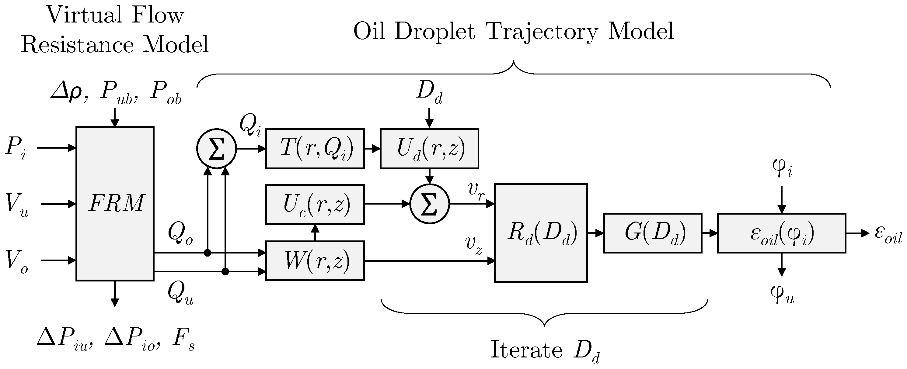
2. Hydrocyclone Model Framework

This section defines the framework of the developed hydrocyclone model. The proposed framework consists of a number of model blocks to differentiate between and identify the predominant system mechanisms. The combined model is illustrated in Figure 5 and executes the following steps:

• Estimate input and output flow rates based on the virtual flow resistance model ($FRM$).
• Estimate carry phase velocity fields.
• Estimate dispersed phase velocity fields.
• Iterate trajectories of dispersed phase.
• Evaluate rejection chance per dispersed phase size class.
• Estimate separation efficiency given inlet dispersed phase size distribution.

The combined model is based on previous work, where step 1 is described in [17], and steps 2–6 are described in [55] and further extended in [56].

The model is designed to estimate the hydrocyclone performance in a broad range of operating conditions. The model is designed to be suitable for:

• Test-bed for controller design.
• Preliminary training for machine learning models.
• Performance evaluation.
• Fault detection and diagnosis.
• Alarm reasoning.
• Root-cause analysis.

The relatively low computational cost enables the model to generate large quantities of training data for learning-based black-box models such as neural networks. As there are always modeling errors, the black-box models can be trained in two stages: (1) training on large amounts of data from the grey-box model and (2) training on data from the designated separation plant. This is especially valuable as running and implementation on the designated separation plant can be expensive and time-consuming. The model can be used as an indicator of the current separation performance, which can also be achieved by measuring the OiW concentration before and after the hydrocyclone. However, measuring real-time OiW concentration has limitations and might even prove to be unreliable, as described in [58]. This idea can be extended to fault detection and diagnosis, alarm reasoning, and root-cause analysis, as the model can be used to derive logical links between operating conditions and their corresponding expected performance.

To fulfill these requirements, the model mechanics are generally derived from first principles wherever computationally convenient, whereas the more complicated fluid dynamic behaviors are described via simplified mathematical equations.

2.1. Virtual Flow Resistance

The first part of the model structure in Figure 5 is a virtual flow resistance model. The principle is to define a simplified pressure drop network and solve it. The hydrocyclone is functionally decomposed into three virtual flow resistances or orifice equations. The decomposition is illustrated in Figure 6.

The main purpose of solving this pressure drop network is to achieve an estimate of $Q_u$ and $Q_o$ with respect to different opening degrees of the control valves $V_o$ and $V_u$. To solve the equations the upstream pressure, $P_i$, and downstream back pressures, $P_{ob}$ and $P_{ub}$, are provided by pressure transmitters. The unknown virtual flow permeability constants: $K_i$, $K_u$, and $K_o$ of the three virtual orifices: $R_i$, $R_u$, and $R_o$ in Figure 6 are obtained by regression on experimental data. The pressure drops are estimated as

$$\Delta P_{ij}=P_i-P_j=\frac{{(Q_u+Q_o)}^2}{K_i},$$

(11)

$$\Delta P_{ju}=P_j-P_u=\frac{Q_u^2}{K_u},$$

(12)

and

$$\Delta P_{jo}=P_j-P_o=\frac{Q_o^2}{K_o}.$$

(13)

Various different valve types and sizes are likely to exist on deoiling hydrocyclone systems, and to accommodate this, the valve equation in this model framework can be substituted by another valve system-specific model. The pressure difference over the valves are assumed as

$$P_u-P_{ub}=\frac{Q_u^2}{{\left(K_{V_u}{V}_u\right)}^2}$$

(14)

and

$$P_o-P_{ob}={\left(\frac{Q_o}{K_{V_{o}1}{V}_o^{\frac{1}{2}}}\right)}^2+\frac{Q_o^2}{K_{V_{o}2}^2}.$$

(15)

The pressure drop over $V_o$ is decomposed into two terms: a variable and a fixed orifice equation. The decomposition was done due to the relatively small diameter of the overflow pipe on the physical pilot plant. The virtual flow resistance model is not complete, with Equations (11)–(15) with the five unknowns: $Q_u$, $Q_o$, $P_j$, $P_u$, and $P_o$, where

$$Q_i=Q_u+Q_o.$$

(16)

An equation that solves $PDR$ can be formulated by substituting Equations (11)–(13), into Equation (8)

$$PDR=\frac{P_i-P_o}{P_i-P_u}=\frac{K_u{K}_o{Q}_i^2+K_u{K}_i{Q}_o^2}{K_u{K}_o{Q}_i^2+K_o{K}_i{Q}_u^2}.$$

(17)

This defines PDR to be monotonically increasing with $F_s$, which is a tendency also observed in literature [16,17].

2.2. Velocity Fields

With the flows and pressures defined, the spatial velocities can be estimated given known hydrocyclone geometry. These velocity fields are time-averaged, time-invariant, and assume rotational symmetric flow round the hydrocyclone’s center axis. The velocity at any point inside the hydrocyclone geometry can be described in three components: tangential, axial, and radial velocity, that are assumed as functions of axial, z, and radial, r, location. The $(r,z)$-coordinate system has $z=0$ at $Z_2$, z increasing towards the underflow, $r=0$ at the center axis, and r increasing radially cf. Figure 4. When convenient to do so, normalized radius will be used $\widehat{r}=r/R_z\left(z\right)$, where $R_z\left(z\right)$ is the inner wall radius. This work utilizes a pilot plant that includes a Colman/Thew-type hydrocyclone with the following dimensions; $D_n/D=0.5$, $D_s/D=0.25$, $D_i/D=0.175$, $D_o/D>0.05$, $L_1/D=1$, $L_3/D=15$, ${\beta }_1={20}^{\circ }$, ${\beta }_2={1.5}^{\circ }$.

2.2.1. Tangential Velocity

The tangential velocity, $T\left(r\right)$, describes how fast the fluid moves around the center axis and is estimated as a function of r. As there are no moving parts or pumps, this spinning motion originates from the fluid being introduced tangentially to the hydrocyclone body. The speed of the fluid at the inlet can be described by the inlet flow divided by the inlet area

$$v_i=\frac{4\frac{Q_i}{2}}{\pi D_i^2},$$

(18)

where $Q_i$ is divided by two, as the inlet flow enters through two rotational-symmetrically placed tangential pipes. The geometry of the pilot plant’s hydrocyclone is substituted into Equation (18) to become

$$v_i=\frac{4\frac{Q_i}{2}}{{0.35}^2\pi {\left(2R_z\left(0\right)\right)}^2}.$$

(19)

The swirling flow in a hydrocyclone can be characterized by a combination of two types of vortices: an inner forced vortex and an outer free/semifree vortex [57]. The modeling done by [57] proposes to model these two vortices by a modified Helmholz law,

$$T\left(r\right)=\frac{v_i\alpha {\left(2R_z\left(0\right)\right)}^n}{r^n},$$

(20)

where $n\in [-1,1]$ is a constant that describes how forced/free the vortex is, from −1 being forced to 1 being free, and $\alpha$ is a velocity loss coefficient due to imperfection.

Another approach is to define the swirling flow as a Rankine vortex, which describe the speed in the two regions, using a characteristic radius, $R_k$, to define the border between the two vortex regions:

$$T\left(r\right)=\left\{\begin{array}{cc}\frac{v_i\alpha \left(2R_z\left(0\right)\right)r}{R_k^2}\hfill & r\le R_k\hfill \\ \frac{v_i\alpha \left(2R_z\left(0\right)\right)}{r}\hfill & r>R_k\hfill \end{array}\right..$$

(21)

It should be noted that $T\left(r\right)$ of the free and forced vortex approach $v_i\alpha \left(2R_z\left(0\right)\right)/R_k$ when $r\to R_k$. An important note, regardless of whether using Helmholz law or Rankine vortex, is that the significant separation occurs in the outer vortex region [57]. Therefore, the model accuracy in the outer region is favored over accuracy near the axis center. It should be noted that Equations (20) and (21) are time-invariant simplifications of the reality, and that hydrocyclones might generate and maintain a proceeding vortex core during operation [59,60]. The proposed model utilizes Equation (20) for estimating $T\left(r\right)$ with its parameters defined in Section 4.

2.2.2. Axial Velocity

The axial velocity describes how fast the fluid moves towards the underflow. In normal operation, this velocity distribution is characterized by being positive near the inner wall where the fluid moves towards the underflow, and negative near the center axis where it moves towards the overflow. All cross-sections orthogonal to the center axis in $S_{2-4}$ have a circle with a specific radius where the axial velocity is zero. These cross-sections must have an equal net flow rate assuming incompressible flow, as the fluid is unable to accumulate. This extrudes the circles of zero axial velocity into a truncated cone or envelope of zero axial velocity. The radius of these circles of zero axial velocity is often referred to as the locus of zero axial velocity [61]. As $R_z\left(z\right)$ is a function of z, it is often convenient to define the axial velocity distribution in normalized radius; $\widehat{r}=r/R_z\left(z\right)$ [55]. An experimental approach is proposed by [57,62], that approximate the axial velocity distribution as a third order polynomial:

$$Y\left(\widehat{r}\right)={\theta }_1+{\theta }_2\widehat{r}+{\theta }_3{\widehat{r}}^2+{\theta }_4{\widehat{r}}^3,$$

(22)

where $\mathbf{\theta }=[{\theta }_1,{\theta }_2,{\theta }_3,{\theta }_4]$ is a set of constants. To get the axial velocity, W, at a given $\widehat{r}$, Equation (22) must be scaled with the net cross-sectional flow rate. In [57], one $\mathbf{\theta }$ is identified for a specific operation condition. However, it is clear that $\mathbf{\theta }$ changes dependent on operation conditions, which is proved by the case where either $V_u$ or $V_o$ closes, causing $F_s$ to change drastically and alter the velocity distributions. This incentivized [56] to propose an analytic solution to $\mathbf{\theta }$ based on four constraints:

• Maximum axial velocity at the inner wall:

  $$\frac{dY\left(\widehat{r}\right)}{d\widehat{r}}{|}_{\widehat{r}=1}=0,$$

  (23)

  constrains $Y\left(\widehat{r}\right)$ to have a local extremum at the hydrocyclone inner wall [56]. This assumes no boundary layer at the wall or that it is infinitesimal. In reality, this boundary layer exists as the fluid speed approaches zero when $\widehat{r}$ approaches one. The slow speed in the boundary layer enables "short-circuiting" of the oil droplets so that they creep along the wall towards the outlets without experiencing separation. However, accounting for the boundary layer in Equation (22) adds more complexity, which might introduce more problems/inaccuracies than it solves, as more constraints are required. Additionally, the effects of the boundary layer are likely insignificant compared to the separation that occurs in the remaining volume and not considered for this work.
• Minimum axial velocity at the center axis:

  $$\frac{dY\left(\widehat{r}\right)}{d\widehat{r}}{|}_{\widehat{r}=0}=0,$$

  (24)

  constrains $Y\left(\widehat{r}\right)$ to have a local extrema at the hydrocyclone center axis [56]. This assumes that the fluid shear stress, $\tau$, is proportional to $\widehat{r}$, such that ${lim}_{\widehat{r}\to 0}\tau =0$ [63]. Some cases have ${lim}_{\widehat{r}\to 0}\frac{dY}{d\widehat{r}}$ approximated as non-zero, as in [57], other cases have it approximated, simulated, or measured as zero [32,47,52,64]. The difference of these two methods is likely small for the droplet trajectory approach, as it mainly affect the velocity very close to the center axis, and becomes increasingly similar with $\widehat{r}$.
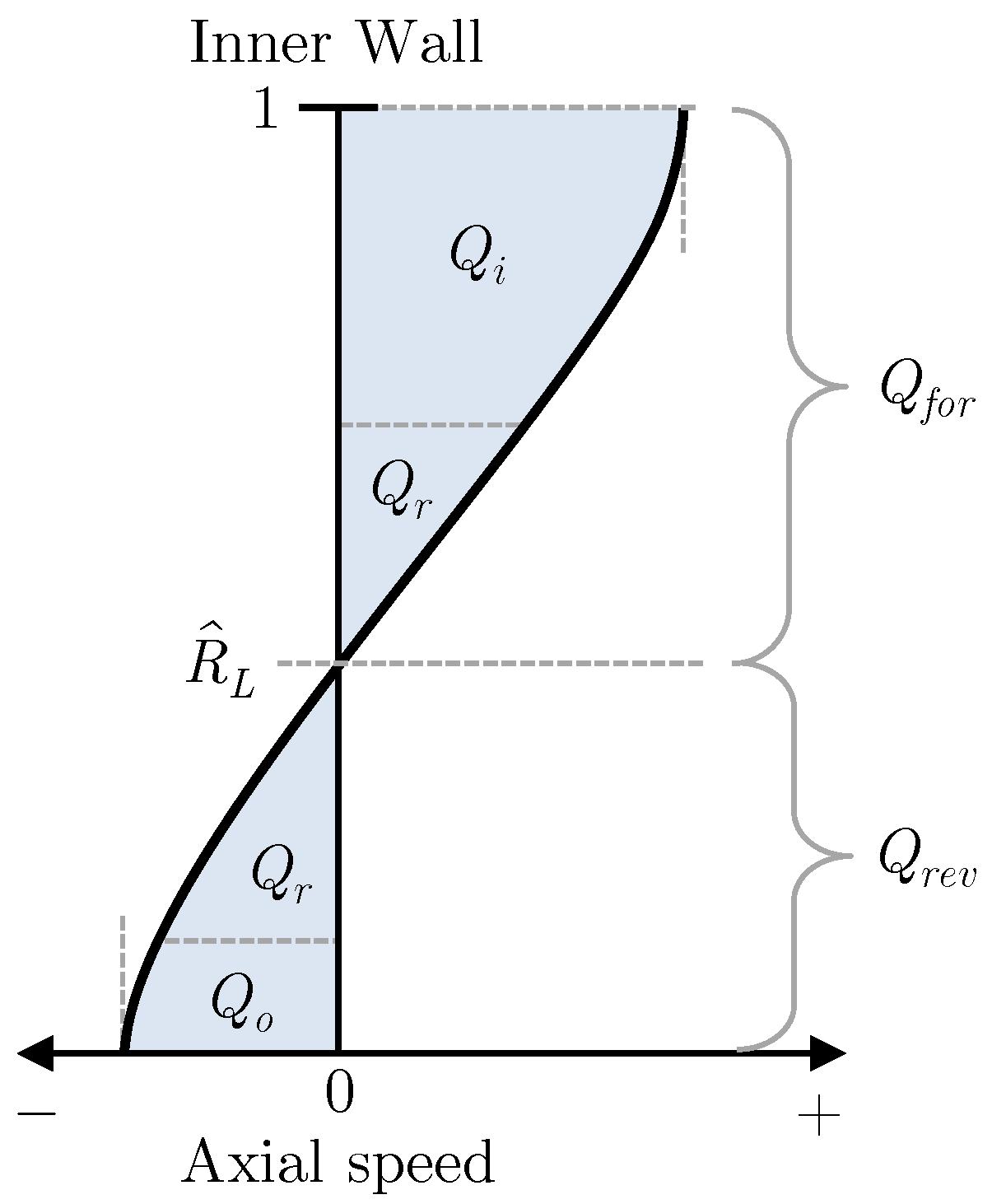
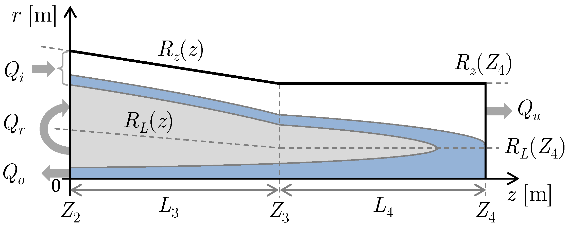
• Volume balance of the forward flow:

  $$Q_{for}=2\pi {\int }_{{\widehat{R}}_L}^{1}Y\left(\widehat{r}\right)\widehat{r}d\widehat{r},$$

  (25)

  where $Y\left({\widehat{R}}_L\right)=0$, $Q_{for}=Q_i+Q_r$, and ${\widehat{R}}_L=\frac{R_L}{R_z}$. This is a mass balance on the outer flow region which borders the envelope of zero axial velocity ($\widehat{r}={\widehat{R}}_L$) and the hydrocyclone inner wall ($\widehat{r}=1$), assuming incompressible flow. The forward flow is illustrated in Figure 7. The part of $Q_{for}$ that recirculates the hydrocyclone, $Q_r$, is also present in the reverse flow, $Q_{rev}$. The phenomenon of a recirculation flow region as well as short circuit flow and how it is reduced by the length of the vortex finder, are well described in [48,61,65].
• Volume balance of the reverse flow:

  $$Q_{rev}=-2\pi {\int }_0^{{\widehat{R}}_L}Y\left(\widehat{r}\right)\widehat{r}d\widehat{r},$$

  (26)

  where $Q_{rev}=Q_o+Q_r$, formulates a mass balance on the inner flow region contained to be inside the envelope of zero axial velocity and also illustrated in Figure 7. The minus sign converts the negative flow rate from integration into being positive, as a result of this work’s flow definitions. As flow across the envelope of zero axial velocity will be introduced later, these two mass balance constraints are only evaluated at $Z_2$, where $z=0$.

Axial mass balance is preserved with the 3rd and 4th constraint, such that

$$Q_u=Q_{for}-Q_{rev}=2\pi {\int }_0^{1}Y\left(\widehat{r}\right)\widehat{r}d\widehat{r},$$

(27)

as

$$Q_u=Q_i+Q_r-(Q_o+Q_r),$$

(28)

at all axial cross-sections. Additional to the four constraints is the definition of ${\widehat{R}}_L$ which implies

$$Y\left({\widehat{R}}_L\right)=0.$$

(29)

With the four constraints defined, the expressions can be simplified by reducing the number of equations and unknowns. As the 1st and 2nd constraint are assumed for all operating conditions, they can be substituted into Equation (22) to reduce the number of unknowns needed to be solved during operation. This implies that

$${\theta }_1=-{\theta }_4{\widehat{R}}_L^3+\frac{3}{2}{\theta }_4{\widehat{R}}_L^2,$$

(30)

$${\theta }_2=0,$$

(31)

and

$${\theta }_3=-\frac{3}{2}{\theta }_4,$$

(32)

such that Equation (22) becomes

$$Y\left(\widehat{r}\right)=-{\theta }_4{\widehat{R}}_L^3+\frac{3}{2}{\theta }_4{\widehat{R}}_L^2-\frac{3}{2}{\theta }_4{\widehat{r}}^2+{\theta }_4{\widehat{r}}^3.$$

(33)

The expression for $Y\left(\widehat{r}\right)$ is substituted into Equations (25) and (26).

Some studies state that $Q_r$ scales with $Q_i$ [48,57,61]. One reason for this scaling is likely due to the boundaries of the $Q_r$ volume, which is typologically similar to a torus, are exposed to friction from the speed of the surrounding fluid. In the approximations of [57], $Q_u$, $Q_o$, and $Y\left(\widehat{r}\right)$ are defined, such that a relationship between the flows can be calculated. The recirculation rate, $R_R$, is calculated in [56] to be

$$R_R=\frac{Q_r}{Q_i}=0.02,$$

(34)

which implies that

$$Q_{for}=(1+R_R)(Q_u+Q_o)$$

(35)

and

$$Q_{rev}=(1+R_R)Q_o+R_R{Q}_u.$$

(36)

Equations (35) and (36) are substituted into Equations (25) and (26), respectively. With these substitutions, Equations (25) and (26) remain with the two unknowns ${\theta }_4$ and ${\widehat{R}}_L$, which are solved in each prediction step during operation using $Q_u$ and $Q_o$ as inputs obtained from the virtual flow resistance model. After Equations (25) and (26) are solved, ${\theta }_4$ and ${\widehat{R}}_L$ are substituted into Equation (22) to get the axial velocity distribution for the current time step. As an example, Figure 8 shows how ${\widehat{R}}_L$ changes as the flow rates change and indicates that ${\widehat{R}}_L$ is proportional to $Q_o/Q_u$.

If computation time is too long, ${\widehat{R}}_L$ can be solved in a grid of flow combinations before operation, and then interpolated during operation. An example of this grid is shown in Figure 8.

The flow regions in $S_{3-4}$ are illustrated in Figure 9, vertical dashed line indicates the border between the two segments, horizontal dashed line is ${\widehat{R}}_L$ throughout the length of the segments.

The definition of these flow regions derives from Equation (16). The three grey arrows on the left in Figure 9 illustrate the mass balance in Equation (28). The total carry phase flow rate that crosses the envelope spanned by $R_L$ is

$$Q_L=Q_r+Q_o,$$

(37)

as $Q_r$ recirculates and $Q_o$ eventually exits the overflow. If $Q_L$ is zero, the axial velocity of the carry phase flow is

$$W(r,z)=\frac{Y\left(\frac{r}{R_z\left(z\right)}\right)}{R_z^2\left(z\right)},$$

(38)

which converts Y into absolute cylindrical coordinates of the $(r,z)$-plane. When $Q_L$ is non-zero, the contribution from $Q_r$ to the cross-sectional flow rate decreases with z, as illustrated as an infinitesimal cell in Figure 10.

Additionally, $Q_o$ is drained from $Q_{for}$ into $Q_{rev}$ near the underflow. If assuming $Q_{rev}$ eventually crosses the envelope spanned by $R_L$, then the average radial velocity of the flow at the envelope is,

$$V_L=\frac{Q_{rev}}{A_L},$$

(39)

where $A_L$ is the total area of the envelope spanned by $R_L$:

$$A_L=\pi {\widehat{R}}_L\left(L_3\left(\frac{D_n+D_u}{2}\right)+L_4{D}_u\right).$$

(40)

The draining does not only affect the flow fields at the envelope, and it is generalized to the rest of the volume to define a radial speed contribution due to draining:

$$U_L(r,z)=-V_L\frac{2\pi R_{L}dz}{2\pi rdz}\frac{{\int }_{\widehat{r}}^{1}2\pi \check{r}Y\left(\check{r}\right)d\check{r}}{Q_{for}}$$

(41)

where the accent ($\stackrel{ˇ}{}$) denotes a integration variable. Equation (41) is reduced to

$$U_L(r,z)=-V_L\frac{R_L}{r}\frac{{\int }_{\widehat{r}}^{1}2\pi \check{r}Y\left(\check{r}\right)d\check{r}}{Q_{for}},$$

(42)

which is a scaling of $V_L$ and illustrated in Figure 11, where the minus sign defines $U_L(r,z)$ to be negative, i.e., moving towards the hydrocyclone center axis.

When $r=R_L$ then $|U_L|=|V_L|$. When $r=R_z$ then $U_L=0$. If $|U_L(r,z)|$ increases then $\left|W\right(r,z\left)\right|$ must decrease, when assuming incompressible flow. To apply this effect to Equation (38), an axial speed scale due to the fluid moving across the envelope, $W_s$, is defined as:

$$W_s\left(z\right)=1-\frac{|V_{L}2\pi {\int }_0^z{R}_L\left(\check{z}\right)d\check{z}|}{Q_{for}},$$

(43)

where $W_s\in [0,1]$, such that Equation (38) becomes:

$$W(r,z)=W_s\left(z\right)\frac{Y\left(\frac{r}{R_z\left(z\right)}\right)}{R_z^2\left(z\right)}.$$

(44)

$W_s=1$ when $z=0$. $W_s$ decreases with z. The formulation of $W(r,z)$ is only valid for $r\ge R_L$. This concludes $W(r,z)$ at all points inside $S_3$ and $S_4$, where $r\ge R_L$.

2.2.3. Radial Velocity

It is common to estimate the radial velocity of the continuous phase as

$$U_w(r,z)=\frac{-r}{R_z\left(z\right)}W(r,z)\tan \left(\frac{{\beta }_2}{2}\right),$$

(45)

which accounts for ${\beta }_2$ of $S_3$ and satisfies continuity [35,56]. As the walls in $S_4$ are parallel, $U_w(r,z)=0$ everywhere in $S_4$. The resulting radial velocity of the carry phase becomes

$$U_c(r,z)=U_w(r,z)+U_L(r,z),$$

(46)

when accounting for the envelope drain. At the wall

$$U_c(R_z\left(z\right),z)=W(R_z\left(z\right),z)\tan \left(\frac{{\beta }_2}{2}\right),$$

(47)

and at the locus

$$U_c(R_L\left(z\right),z)=U_w(R_L\left(z\right),z)+V_L.$$

(48)

For all modeling purposes, the droplets follow the same velocity fields as the water, except for one additional radial component by from settling speed via Stokes law

$$U_d(r,D_d)=-\frac{\Delta \rho D_d^{2}T{\left(r\right)}^2}{18\mu r},$$

(49)

where the minus sign directs this speed towards the hydrocyclone center axis. The radial speed of oil droplets is then equal to $U_c+U_d$. The literature generally agrees that it is fair to assume that Equation (49) is the only velocity difference between the carry phase water and the dispersed oil droplets [23,57].

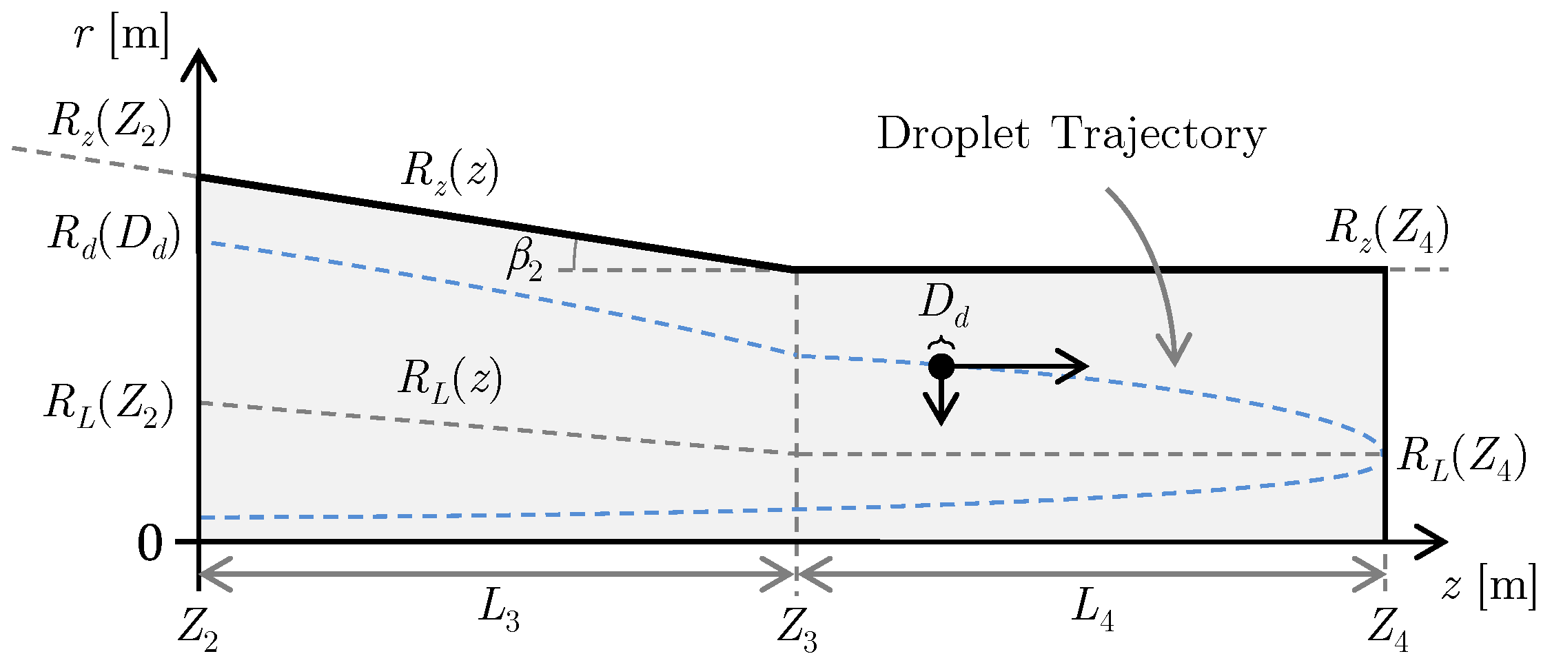
2.3. Droplet Trajectory

The combined velocity fields in tangential, axial, and radial direction for an oil droplet with size $D_d$ are summarized as

$$\left[\begin{array}{c}{v}_T\\ v_r\\ v_z\end{array}\right]=\left[\begin{array}{c}T\left(r\right)\\ U_c(r,z)+U_d(r,D_d)\\ W(r,z)\end{array}\right].$$

(50)

Computing the droplets trajectory following Equation (50) returns a helix-like line with varying radius. As the number of rotations a droplet experiences is insignificant information for evaluating whether the droplet leaves the underflow or overflow, angular position can be disregarded to reduce computation. This reduces the relevant velocities to be axial and radial in the $(r,z)$-plane:

$$\left[\begin{array}{c}{v}_r\\ v_z\end{array}\right]=\left[\begin{array}{c}{U}_c(r,z)+U_d(r,D_d)\\ W(r,z)\end{array}\right].$$

(51)

Droplet trajectories can now be computed given an initial position in the $(r,z)$-plane by updating the position using Equation (51) with appropriate time steps. A droplet is assumed to enter $S_3$ in the outer-most ring marked with $Q_i$ in Figure 9. A droplet is assumed separated and leaves the overflow if its radial position becomes less than $R_L\left(z\right)$ and assumed not separated if its axial position exceeds $L_3+L_4$. Based on this assumption, the critical trajectory of a specific droplet size is defined as the trajectory that crosses the point $(R_L\left(Z_4\right),Z_4)$ as shown in Figure 12. The critical trajectory has the starting radial position at $Z_2$ named $R_d\left(D_d\right)$.

It is assumed that a droplet with size $D_d$ that

• starts outside $R_d\left(D_d\right)$ will leave the underflow, or
• starts inside $R_d\left(D_d\right)$ will leave the overflow.

Some of the droplets will be separated by simply splitting the inlet flow. This is illustrated by the $Q_o$ region in Figure 9. This is relevant for definition of separation efficiency, as in Equations (9) and (10). $R_d\left(D_d\right)$ is found by computing the critical trajectory starting from $(R_L\left(Z_4\right),Z_4)$ using negative time steps. $R_d$ needs to be found for a range of droplet sizes, as droplet size is a distribution. This can be done by computing $R_d\left(0\right)$, and then increase the droplet size in discrete increments, until $D_{d_{100}}$ is found when $R_d\left(D_{d_{100}}\right)\ge R_z\left(Z_2\right)$. By this definition, droplets larger than $D_{d_{100}}$ will always be separated. As a result, trajectories with droplets larger than $D_{d_{100}}$ are not computed.

2.4. Grade Efficiency

It is convenient to utilize the definition of $R_d$ when estimating G, as $R_d\left(D_d\right)$ establishes the notion of whether a droplet becomes separated or not, given the droplets starting point. The remaining question becomes; what is the distribution of droplet trajectory starting positions? Some studies have the droplets to be uniformly distributed in the area of a hollow disk with minimum radius $R_L\left(0\right)$ and maximum radius $R_z\left(0\right)$ at the start of $S_3$ [57]. G is in that case a ratio between the area of the hollow disk from $R_d\left(D_d\right)$ to $R_z\left(0\right)$ and the area of the hollow disk from $R_L\left(0\right)$ to $R_z\left(0\right)$, such that

$$G_{area}\left(D_d\right)=\left\{\begin{array}{cc}\frac{\pi R_d{\left(D_d\right)}^2-\pi R_L{\left(0\right)}^2}{\pi R_z{\left(0\right)}^2-\pi R_L{\left(0\right)}^2}\hfill & \mathrm{if}{D}_d\le D_{d_{100}}\hfill \\ 1\hfill & \mathrm{otherwise}\hfill \end{array}\right..$$

(52)

However, consider a unit starting area that has twice the axial velocity of another unit starting area. This unit of area would then have twice the amount of fluid passing through. With the assumption that droplets are uniformly distributed in volume, Equation (52) must be updated to account for how the axial velocity is distributed across the hollow disk from $R_L\left(0\right)$ to $R_z\left(0\right)$:

$$G_{vol}\left(D_d\right)=1-\frac{2\pi {\int }_{\frac{R_d\left(D_d\right)}{R_z\left(0\right)}}^1\widehat{r}Y\left(\widehat{r}\right)d\widehat{r}}{Q_i}.$$

(53)

It should be noted that

$$G_{vol}\left(0\right)=1-\frac{Q_u}{Q_i}=\frac{Q_o}{Q_i}=F_s,$$

(54)

which represent the amount of droplets removed by simply splitting the flow. If ${\phi }_i$ is known, then ${\phi }_u$ can be found by

$${\phi }_u=G_{vol}{\phi }_i.$$

(55)

It should be noted that ${\phi }_u$ does not sum to one in Equation (55) but rather ${\epsilon }_{oil}$, which can be useful for performance evaluation purposes. The majority of ${\phi }_i$ is commonly 5–60 µ$\mathrm{m}$ [22,57].

2.5. Total Efficiency

The efficiency defined in Equations (9) and (10) depends on G and ${\phi }_i$. The total volumetric percentage of inlet oil that leaves the overflow can be calculated as

$${\epsilon }_{oil}={\int }_0^{\infty }{G}_{vol}\left(D_d\right){\phi }_i\left(D_d\right)d{D}_d.$$

(56)

As $G_{vol}=1\forall D_d>D_{d_{100}}$, Equation (56) can be divided into two terms

$${\epsilon }_{oil}={\int }_0^{D_{d_{100}}}{G}_{vol}\left(D_d\right){\phi }_i\left(D_d\right)d{D}_d+{\int }_{D_{d_{100}}}^{\infty }{\phi }_i\left(D_d\right)d{D}_d.$$

(57)

The downside of this estimation of ${\epsilon }_{oil}$ is that it requires a known ${\phi }_i$. In the cases where ${\phi }_i$ is not available, specific points on $G_{vol}$ can be used as a performance indicator, such as $D_{d_{50}}$ defined by

$$G_{vol}\left(D_{d_{50}}\right)=50\%,$$

(58)

which is the diameter of a droplet which has a 50% chance of leaving the overflow given the current operation conditions.

3. Hydrocyclone Model Parameters and Operation

The parameters for the model can be classified based on how they are obtained. These parameters are found once, as a part of the initialization, and are from: fluid properties, hydrocyclone design specifications, estimations, or empirical studies.

3.1. Geometrical Parameters

These parameters are either provided by the manufacturer of the hydrocyclone or directly measured. As these lengths are internal, they can be inconvenient to directly measure without disassembly. The geometrical parameters are: $D_{i,n,u}$, $L_{3,4}$, and ${\beta }_2$. These parameters are assumed to be constant throughout the operation. However, especially the diameters may change slowly over time due to sand erosion or sediment deposition.

3.2. Estimated Parameters

Some parameters require a data set of measured $P_{i,u,o,ub,ob}$ and any two measurements of $Q_{i,u,o}$ to be estimated. These parameters are from the virtual flow resistance model: $K_{i,u,o,V_u,V_{o}1,V_{o}2}$. It should be noted that the pressure measurements can also be fulfilled using pressure difference measurements over the valves and the hydrocyclone. Additionally, the structure of Equation (14) and (15) can be changed to accommodate valve characteristics, which for this work included the parameters: $K_{V_u,V_{o}1,V_{o}2}$.

3.3. Empirical Parameters

These parameters are used in estimating the velocity fields, and are: $\alpha$, n or $R_k$, and $R_R$. These parameters could be estimated, but they require either sophisticated simulation or intrusive measurements to be obtained. The complete list of model parameters is summarized in

Table 1. Summary of model parameters.

Symbol	Value	Unit	Source	Method
Fluid Parameters:
${\rho }_{oil}$	850	$\frac{\mathrm{kg}}{{\mathrm{m}}^3}$	-	Look-up
${\rho }_{water}$	999	$\frac{\mathrm{kg}}{{\mathrm{m}}^3}$	-	Look-up
${\mu }_{water}$	$1.002·{10}^{-3}$	$\frac{\mathrm{kg}}{\mathrm{m}·\mathrm{s}}$	[63]	Look-up
Geometrical Parameters:
$R_z\left(Z_2\right)$	10	$\mathrm{mm}$	-	Manufacturer
$R_z\left(Z_3\right)$	5	$\mathrm{mm}$	-	Manufacturer
${\beta }_2$	1.5	${}^{\circ }$	-	Manufacturer
$L_2$	0.382	$\mathrm{m}$	-	Manufacturer
$L_3$	0.6	$\mathrm{m}$	-	Manufacturer
Estimated Parameters:
$K_i$	437	$\frac{{\mathrm{L}}^2}{\mathrm{bar}·{\mathrm{s}}^2}$	[17]	Regression
$K_u$	4219	$\frac{{\mathrm{L}}^2}{\mathrm{bar}·{\mathrm{s}}^2}$	[17]	Regression
$K_o$	0.264	$\frac{{\mathrm{L}}^2}{\mathrm{bar}·{\mathrm{s}}^2}$	[17]	Regression
$K_{V_u}$	31.346	$\frac{{\mathrm{L}}^2}{\mathrm{bar}·{\mathrm{s}}^2}$	-	Regression
$K_{V_{o}1}$	1.842	$\frac{{\mathrm{L}}^2}{\mathrm{bar}·{\mathrm{s}}^2}$	-	Regression
$K_{V_{o}2}$	0.9856	$\frac{{\mathrm{L}}^2}{\mathrm{bar}·{\mathrm{s}}^2}$	-	Regression
Empirical Parameters:
$\alpha$	0.5	-	[57] with [23]	Laser Doppler anemometry
n	0.65	-	[57] with [23]	Laser Doppler anemometry
$R_R$	0.02	-	[56] with [57]	Mass balance

.

This concludes the model structure and its associated parameters.

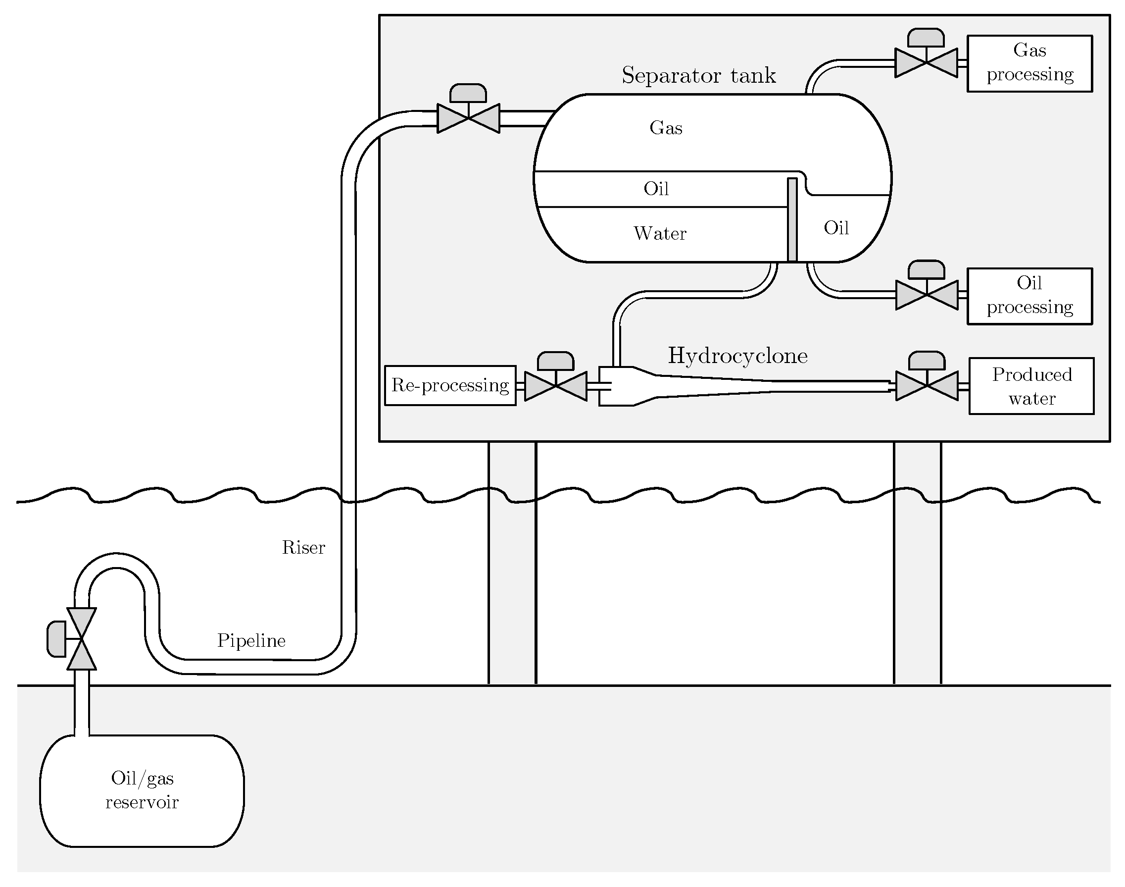
4. Experiment Facility

This section describes the experimental setup used for model validation. The testing facility used for this work is based on the pilot plant described in [66]. The hydrocyclone subsystem of the plant was modified to obtain better OiW concentration measurements by complying with good sampling practices compared to [67]. An illustration of the modified hydrocyclone subsystem of the pilot plant can be seen in Figure 13.

The modified subsystem is a commonly used hydrocyclone setup with underflow and overflow valves, with sidestreams located on the inlet and underflow stream. In this setup, each sidestream is equipped with two OiW monitors, a flow meter, and a control valve. The inlet sidestream is configurable to return the flow to the mainstream by opening $V_R$ and closing $V_D$ or to discard the flow to the supply tank by opening $V_D$ and closing $V_R$. In this subsystem, all control valves are Bürkert 8802-GD-I pneumatic valve systems. The feed pump, $WP$, is a Grundfos CRNE 5-9 centrifugal pump. Two Milton Roy Mixing HELISEM VRP3051S90 mixers continuously stir fluid in the supply tank, which consists of a non-detergent SAE30 Midland oil and filtered tap water emulsion. The critical measurements for this experiment include two Turner Design TD-4100XDC fluorescence-based OiW monitors at the sidestreams of the hydrocyclone inlet to measure $C_i$ and on the underflow to measure $C_u$. These monitors were used and calibrated similarly to [68]. Three Rosemount electromagnetic flow meters are located at the inlet and underflow as well as underflow sidestream to measure $Q_i$, $Q_u$, and $Q_{us}$. A Coriolis flow meter is used to measure $Q_{is}$ Pressure transmitters are deployed at various locations to measure all the relevant pressures of this system. Features gained from the subsystem modification includes:

• Vertical sampling.
• Facilitate flow or delta pressure control.
• Interchangeable sampling probes.
• Redundant OiW monitors.
• Short distance from the probes to the OiW monitors.

The lighter phase tends to settle at the top of horizontal pipes and will create a vertical concentration polarization, which may cause unfair sampling. This polarization effect is eliminated by vertical sampling. The manufacturer of the OiW monitors states that the sidestream flow rate must be maintained in the range of 1–3 $\mathrm{L}/\min$. To facilitate this, the sidestream valves $V_{is}$ and $V_{us}$ can be actuated by a controller using the measured sidestream flow rate from $Q_{is}$ and $Q_{us}$ as feedback. The control of the sidestream valves also enables the sidestream flow to be sampled isokinetically at the sample probe. Two OiW monitors were installed at each sidestream to have redundant comparable OiW concentration measurements. This is a desired feature, as several effects can cause an OiW monitor to become unreliable. As it is normal for fluid to travel at a much slower velocity in the sidestream compared to the mainstream, the length from the probe to the OiW monitor introduces significant delay. To reduce this effect, the OiW monitors are located immediately after the probes, such that the travel length from the probe to the first monitor is ∼20 $\mathrm{cm}$.

To enable flow through the sidestreams, the valves $V_i$ and $V_{ub}$ can be choked to generate delta pressure over the sidestreams. This delta pressure can be considered the operational cost of utilizing sidestreams. The inlet sidestream modes are:

• Return: this mode returns the flow to the mainstream and can be considered less intrusive as it does not subtract/drain flow from the mainstream. Delta pressure cost is high as a result of choking $V_i$.
• Discard: this mode discards the flow to the supply tank and is operationally cheaper as the pressure difference is sufficient and allows $V_i$ to be fully open. However, if the sampling is unfair, i.e., it extracts a higher or lower OiW concentration than the mainstream, the mainstream concentration will be affected.

5. Experiment Design

The purpose of the experiments was to validate the performance of the proposed hydrocyclone model. Different from [56], the experiment was specifically designed to avoid the flow dependencies of the OiW monitors, as described in [58]. The experiments are divided into three types, where the first type relates to deploying the OiW monitors, the second type relates to preparing the system for the circulation of the OiW mixture, and the third type relates to designing validation experiments for the proposed grey-box model.

5.1. Preparing Real-Time OiW Measurements

Online fluorescence-based OiW monitors were used for all the executed experiments to measure $C_i$ and $C_u$ to provide a real-time estimate of $\epsilon$. Good practices for general online monitoring of OiW are described in [69]. The four OiW monitors’ sensitivities were adjusted, such that half of the output range was ∼250 $\mathrm{ppm}$, which sets up the monitors to measure OiW concentrations from 0–500 $\mathrm{ppm}$. As the setup uses filtered tap water as the water phase, the four OiW monitors were calibrated using the filtered tap water, according to the manufacturer’s recommendations of using the carry phase as the blank sample. To identify the calibration curve, 18 points were collected by injecting six samples of known concentrations three times into each of the four OiW monitors. The known concentrations were $0,10,25,100,250,$ and 400 $\mathrm{ppm}$. The linear calibration curve that translates relative fluorescence units RFU into ppm was identified using least squares regression.

Previous works that investigated the performance of the OiW monitors concluded a set of operational variables that affect the concentration measurement of the chosen OiW monitor, without necessarily altering the mainstream OiW concentration and thus leads to unfair OiW measurements [58]. To avoid affecting the OiW measurement unfairly, the experiments are recommended to comply with these restrictions:

• Sidestream flow rates within manufacturer limits.
• Constant pump speed.
• Constant mainstream flow rate.

To comply with the first restriction, $V_{is}$ was manipulated by a controller that uses $Q_{is}$ as feedback to maintain a constant flow rate of $1.5$$\mathrm{L}/\min$. Similarly, $V_{us}$ was manipulated by a controller that uses $Q_{us}$ as feedback to maintain a constant flow rate of $1.5$$\mathrm{L}/\min$. Additionally, $V_i$ and $V_D$ were fully open and $V_R$ was fully closed to facilitate higher mainstream flow rates.

5.2. Preparing System Mixture

The purpose of this experiment was to prepare a mixture in the supply tank that emulates a realistic inlet concentration for deoiling hydrocyclones in normal operation. Oil was added to the supply tank, and continuously stirred by the mixers, while the system recycled the mixture. $V_o$ was closed to disable separation effects from the hydrocyclone. Experiment settings:

• $WP$ was running constantly at $100\%$ speed.
• $V_{ub}$ was manipulated by a controller that uses $P_{ub}$ as feedback to maintain a constant pressure of $2.75$$\mathrm{bar}$.
• $V_u$ was fully open.
• $V_o$ was closed to disable hydrocyclone separation effects.

This experiment was executed several times, with various durations between from 1–5 h, to investigate the long term variations of measured OiW concentration. To investigate the OiW concentration during different time scales, the OiW concentration was observed hourly and daily, after adding oil, and after periods of inactivity.

5.3. Model Performance Experiments

The purpose of this experiment was to compare the estimated ${\epsilon }_{oil}$ from measurements and the model. A short and long grid experiment were performed with a similar approach as in [17]. The purpose of the short grid experiment was to get an understanding of the OiW concentration measurements, the various settling times, and transient responses. The purpose of the long grid experiment was to get a higher resolution grid with a longer time allocated for initialization and the various valve steps. With these recommended operational constraints, the short grid experiment was designed such that:

• $WP$ was constantly running at $100\%$ speed.
• $V_{ub}$ was manipulated by a controller that uses $P_{ub}$ as feedback to maintain a constant pressure of $2.75$$\mathrm{bar}$.
• $V_u$ had a constant opening percentage during each segment.
• $V_o$ was stepped from $0.5\%$ to $97\%$ open with a total of 15 steps maintaining each step for 35 $\mathrm{s}$.
• The sensor outputs, from the last 10 $\mathrm{s}$ of each step, were averaged to obtain the steady state values.
• The first step was maintained for an additional 100 $\mathrm{s}$ to function as initialization that allows the system to reach steady state.
• Before and after the stepping time-window, $V_o$ was closed, and the hydrocyclone was bypassed for a time-window of 180 $\mathrm{s}$, where no separation occurs.

This stair-case-like segment was executed 11 times, each with a different opening of $V_u$ from $25\%$ open to $97\%$. The duration of one segment of this experiment was 180 $\mathrm{s}+100$$\mathrm{s}+15(35$$\mathrm{s})+180$ $\mathrm{s}=985$ $\mathrm{s}$. The long grid experiment was designed similarly, but with the following differences:

• The time-windows of no separation were 300 $\mathrm{s}$ instead of 180 $\mathrm{s}$.
• The first step was maintained for an additional 400 $\mathrm{s}$ instead of 100 $\mathrm{s}$.
• Each $V_o$ step was maintained for 40 $\mathrm{s}$ instead of 35 $\mathrm{s}$.
• 24 h prior to running the long grid experiment, additional oil was added, and the mixers engaged to continually stir at constant speed.

The duration of one segment of this experiment was 300 $\mathrm{s}+400$$\mathrm{s}+15(40$$\mathrm{s})+300$$\mathrm{s}=1600$$\mathrm{s}$.

6. Results

This section describes the results obtained from the designed experiments. The experiment results are divided into the same three types as the experiment design. Firstly, this section will describe calibrating the OiW monitors and validating the OiW monitors’ performance, then provide examples from running the system and observing how the measured OiW concentration changes, and finally, this section compares the model’s predictions to the experiment’s measurements.

6.1. Preparing Real-Time OiW Measurements

The obtained calibration curves based on data from injecting known OiW concentrations into the four OiW monitors can be seen in Figure 14.

Even though the four calibration curves are different, they align well with their individual data points, i.e., the same known injected concentration is likely to be read as four different RFU values, but four very similar ppm values.

6.1.1. Validate Calibration Curve

After running the system for a week with more than 20 h of recirculating the supply tank OiW mixture, it was of interest to validate the calibration by injecting a known OiW concentration into all of the four OiW monitors. To do this, the OiW monitors were removed from the flow loop and injected with a mixture of 0 $\mathrm{ppm}$ blank sample, followed by a mixture of 250 $\mathrm{ppm}$. The measured OiW concentrations during this experiment are shown in Figure 15.

The four monitors’ measured ppm were reasonable and similar for the injected mixtures. However, the output of $C_{i1}$ was less than the three others for the injected mixture of 250 $\mathrm{ppm}$. After flushing the sidestreams by fully opening $V_{is}$ and $V_{us}$, and closing $V_{ub}$, the low reading was no longer observed.

6.1.2. OiW Location Switching

During recirculation of the mainstream flow without separation effects by having $V_o$ closed, it is expected that the four OiW monitors output similar values. However, there was a significant discrepancy between the four OiW measurements, where the largest difference was between the inlet and the underflow OiW monitors.

To test if this was due to faulty calibration, two of the OiW monitors were physically switched, such that the monitor that measured $C_{i2}$ now measures $C_{u2}$ and vice versa. Figure 16 shows the four measured concentrations prior to and after physically switching the two monitors.

It should be noted that the experiment in Figure 15 was performed prior to switching, but after the experiment in Figure 16a. There was no addition nor removal of oil between the experiments in Figure 16a,b. It should also be noted that the post switching experiment was executed two days after the prior switching experiment.

6.2. Preparing System Mixture

This section is dedicated to preparing a fair inlet concentration to the hydrocyclone system.

6.2.1. Long Term Concentration Settling

A common observation from running this experiment was that, after adding oil to the mixture in the supply tank, the measured OiW concentration immediately increased to some value but then continued to decrease over time for up to 7 h before settling. To avoid unmixed oil to enter the sidestreams, and potentially foul the view cell, the mixture was recycled for 1 h using only the mainstream, while $V_{is}$ and $V_{us}$ remain closed. An example of how the OiW concentration decreased over time is shown in Figure 17, where the experiment started after 1 h of mainstream recirculation.

$V_o$ was toggled from fully open to fully closed every 100 $\mathrm{s}$ to investigate all four OiW concentrations during no separation when $V_o$ is closed, as well as introducing the OiW mixture to the overflow pipes.

6.2.2. Dead Volumes

Every T-junction that allows reconfiguration and every pipe section with dead ends creates unintentional volumes where the flow speed is zero. This potentially allows droplets to settle over time. A change in the mainstream flow rate can cause these dead volumes to either deposit or release resting oil, leading to unintentional correlation effects between flow rate and measured OiW concentration. Even though $V_o$ can be closed, the piping at the overflow could potentially deposit significant amounts of oil. To investigate this effect, a direct connection between the inlet and underflow was made and tested, as seen in Figure 18.

To ensure the same flow rate through both configurations, with $WP$ running at $100\%$ speed, $V_i$ was fully open when operating the hydrocyclone and $48\%$ open when bypassing the hydrocyclone. During this experiment, the measured inlet OiW concentration remained similar, while the measured underflow OiW concentration was generally 10 $\mathrm{ppm}$ lower when operating the hydrocyclone.

6.2.3. Common Sidestream

To test all four OiW monitors measuring the same OiW mixture, $C_{u1}$ and $C_{u2}$ were connected in series with $C_{i1}$ and $C_{i2}$. This was physically done by connecting a hose between the output of the monitor measuring $C_{i2}$ and the input of the monitor measuring $C_{u1}$. The measured OiW concentration from all four OiW monitors during this experiment is shown in Figure 19.

As the four monitors share a common sidestream, they are expected to measure identical OiW concentrations. It should be noted that the height difference between the start and end points of the hose connection is about $-1.5$$\mathrm{m}$, as a result of the facility’s design. During the experiment, $C_{i1}$ was similar to $C_{u2}$ and $C_{i2}$ was similar to $C_{u1}$. The observed difference between these two similarities is ∼10 $\mathrm{ppm}$. As the four OiW monitors are in series, the highest absolute pressure is at $C_{u1}$ and the lowest pressure at $C_{u2}$. Additionally, all four OiW monitors share the same sidestream flow rate. In terms of height, the monitors measuring $C_{i1}$ and $C_{u1}$ are equal and the monitors measuring $C_{i2}$ and $C_{u2}$ are equal.

6.3. Model Performance Experiments

This section compares the measured and predicted system variables. The first part presents the measured and predicted values of a segment in the short grid experiment by observing time series, and the last part presents the measured and predicted steady state values of the long grid experiment.

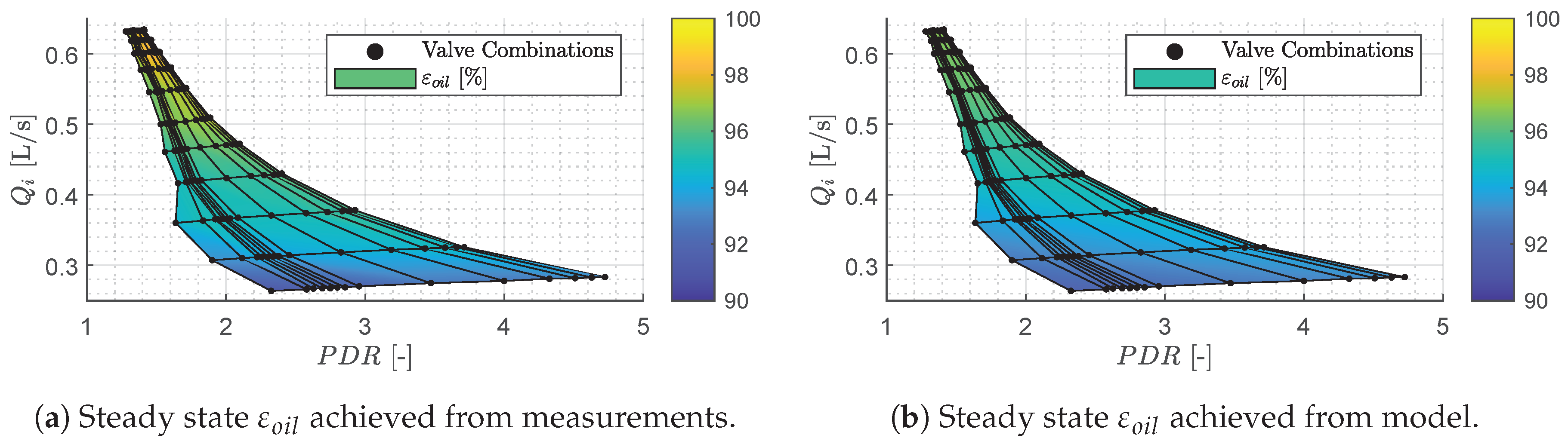
6.3.1. Short Grid Experiment

An abrupt change in $C_u$ is observed when the hydrocyclone is toggled to be bypassed at 180 $\mathrm{s}$ and 805 $\mathrm{s}$, as seen in Figure 20. This indicates that separation occurs inside the hydrocyclone and that this requires a positive non-zero opening of $V_o$. At the no separation time-windows from 0–180 $\mathrm{s}$ and from 805–985 $\mathrm{s}$, all of the OiW monitors should ideally output identical ppm values. In these time-windows, the underflow concentration measurements are ∼25 $\mathrm{ppm}$ higher than the inlet measurements. During the $V_o$ stepping time-window from 280–805 $\mathrm{s}$, there is only a small 10 $\mathrm{ppm}$ change in measured underflow OiW concentration, as seen in Figure 21, and the largest difference in measured underflow OiW concentration occur from zero to the smallest non-zero $V_o$ opening.

It should be noted that the mean inlet droplet size has a considerable impact on the model’s estimated ${\epsilon }_{oil}$. If a small mean droplet diameter causes ${\epsilon }_{oil}$ to be reduced, and implicitly, a larger mean droplet size causes the model’s estimated ${\epsilon }_{oil}$ to be increased. Therefore, it is not the absolute value of ${\epsilon }_{oil}$ that should be compared, but rather, the trends.

In conclusion, the OiW monitors’ output agreed in pairs, i.e., the two inlet measurements are similar, and the two underflow measurements are similar. The measured OiW concentrations in the system have significant long term settling, that must be addressed or accounted for when using these measurements.

6.3.2. Long Grid Experiment

The measured flow rate at the inlet and overflow, during the long grid experiment, are shown in Figure 22a,b, respectively.

$Q_i$ was observed to be significantly dependent on $V_u$, and that both $V_u$ and $V_o$ affect $Q_o$. The $PDR$ from the three pressure measurements $P_i$, $P_u$, and $P_o$ are shown in Figure 23.

The estimated ${\epsilon }_{oil}$ from measurements can be seen in Figure 24a and is generated using

$${\epsilon }_{oil}=1-\frac{\frac{C_{u1}+C_{u2}}{2}{Q}_u}{\frac{C_{i1}+C_{i2}}{2}{Q}_i},$$

(59)

with measurements from the six sensors: $C_{i1}$, $C_{i2}$, $C_{u1}$, $C_{u2}$, $Q_u$, and $Q_o$. It should be noted that the first step of the 11 segments, was discarded due to the actual opening of $V_o$ being inconsistent at openings <$0.6\%$, rendering the resulting grid 11-by-14.

Notably, this estimation does not require the knowledge of droplet size distributions, as it is based on measured OiW concentrations. The time periods before and after the stepping time-window were used to find the average offset between the OiW concentration measurements at the inlet and underflow of each segment. This offset was applied to the underflow OiW concentration measurements, such that inlet and underflow OiW concentrations were similar during no separation.

The highest ${\epsilon }_{oil}$ from measurements appears as if it has a maximum, as observed in Figure 24a. This does not occur with the model as seen in Figure 24b, where ${\epsilon }_{oil}$ approaches a plateau as $V_u$ increases.

Estimated ${\epsilon }_{oil}$ from measurements and the model can also be compared as a function of $Q_i$ and $PDR$ as shown in Figure 25.

Every valve combination from the long grid experiment is represented by black dots and the color-indicator presents the ${\epsilon }_{oil}$ in Figure 25. Generally, the measurements and the model share similar tendencies, with $Q_i$ being an important variable for ${\epsilon }_{oil}$. There is also a slight tendency that higher $PDR$ leads to higher ${\epsilon }_{oil}$, but this trend is significantly weaker than the effect of $Q_i$ on ${\epsilon }_{oil}$.

7. Discussion

This section discusses the results obtained from the designed experiments and the model’s performance. This discussion is divided into three parts. Firstly, this section will discuss the use and calibration of the OiW monitors, then the issues related to the OiW mixture in the system, and finally the model’s prediction performance.

7.1. OiW Measurement Considerations

A general and comprehensive overview of the issues related to measuring OiW concentration using fluorometry is described in detail in [58]. This section will address the calibration and validation thereof.

As observed in Figure 14, the variation in RFU of each standard OiW concentration is relatively small for each individual monitor, with the main difference being the slope, which is a result of the position of each OiW monitor’s sensitivity screw. As the obtained calibration curves translate RFU into ppm, their respective RFU values are allowed to be different, as long as the RFU of injected standard OiW samples cause the OiW monitors to output the same ppm value.

In order to validate the calibration, the monitors were injected with filtered tap water followed by an OiW sample of 250 $\mathrm{ppm}$. The output of $C_{i2}$, $C_{u1}$, and $C_{u2}$, are close to the 250 $\mathrm{ppm}$, while $C_{i1}$ is ∼30 $\mathrm{ppm}$ below the target as seen in Figure 15. However, this OiW monitor did reach 0 $\mathrm{ppm}$ when the blank was injected, which could indicate that its view cell was in a cleaner state than the others. The lower reading of $C_{i1}$ could also be due to sample uncertainty of the produced 250 $\mathrm{ppm}$ sample. In other experiments, $C_{i1}$ and $C_{i2}$ are generally in good agreement, such as in Figure 19.

Figure 16a shows that the measured inlet OiW concentration is higher than the underflow during the experiment. The difference in the measured OiW concentrations are likely due to the effects listed in Section 7.2, as the OiW monitors had been proven capable of outputting similar OiW concentrations in Figure 15. To obtain additional validation of calibration, the monitors measuring $C_{i2}$ and $C_{u2}$ were physically switched and then tested, as seen in Figure 16b. During this experiment, the two underflow OiW monitors are in good agreement, but they are now higher than the measured inlet OiW concentrations. The concentration from the two inlet monitors has dropped ∼100 $\mathrm{ppm}$ between the two experiments, and the underflow OiW concentration measurement has increased 20–30 $\mathrm{ppm}$. These differences are very likely due to a combination of the effects listed in Section 7.2. However, as the inlet and underflow OiW monitors agree in pairs, the calibrations are deemed acceptable.

7.2. Preparing System Mixture

Multiple effects have been considered to affect the OiW measurements in the experimental setup other than the separation effects of hydrocyclone, such as

• Oil accumulating or being freed from surfaces.
• Oil accumulating or being freed from dead volumes.
• Fouling and cleaning of the OiW monitors’ view cell.
• The natural separation versus forced mixing in the supply tank.
• The effects of using T-junctions as sidestream sampling probes.
• Variations in shearing causing variations in droplet size distribution.
• Contamination and microbiological growth.

These listed effects may cause the measured OiW concentrations of the sidestreams to diverge from the true OiW concentrations of the mainstream. In Figure 17, the measured OiW concentration slowly decreases and has not settled after more than 3 h plus 1 h of mainstream circulation. The OiW concentration in the underflow, when $V_o$ is open, remains constant at ∼30 $\mathrm{ppm}$ during the experiment in Figure 17, which indicates that a significant portion of the oil leaves through the overflow. The slow OiW concentration decline could indicate that the oil is slowly being deposited in the system until an equilibrium is reached at the given flow rate. The deposit of oil could potentially be on all system surfaces in contact with the mixture and in the dead volumes of the system’s flow loop. It should also be noted that the measured underflow OiW concentration is higher compared to the inlet during the periods of no separation, which is suspected to be caused by the OiW monitors’ different states of fouling. In Figure 18 the difference between the direct connection to the underflow and using the hydrocyclone with closed $V_o$ is seen. The inlet concentrations are relatively steady at ∼270 $\mathrm{ppm}$ while the concentration measured at the underflow drops ∼10 $\mathrm{ppm}$ whenever the hydrocyclone is used compared to the hose, which could indicate that the closed-off overflow pipe section could be considered as a dead volume. In Figure 19, all four OiW monitors have been connected in series with a hose connecting $C_{i2}$ to $C_{u1}$. In this experiment, the OiW monitors agree in pairs, but this time $C_{i1}$ is similar to $C_{u2}$ and $C_{i2}$ similar to $C_{u1}$, where the difference between the two groups is 10 $\mathrm{ppm}$. The monitors generally agree, which indicates that the general tendency of the measured underflow concentration being higher than the inlet, could be caused by the system and not the OiW monitor view cell fouling state.

During all the experiments, the flow was turbulent in the vertical pipe segments where the sidestream flow is extracted. However, there are sampling issues related to using T-junctions to extract the sidestream flow. Isokinetic sampling probes could be valuable to investigate for future experiments to reduce the effect of sample extraction related issues. The effects of natural separation versus forced mixing in the supply tank, droplet size changes, contamination, and microbiological growth are all likely to affect the OiW measurements and also relevant for future measurement sensitivity investigations.

7.3. Grey-Box Model Performance

This section discusses the experimental validation of the grey-box model. The tested model substructure essentially transforms $Q_u$, $Q_o$, and ${\phi }_i$ into ${\epsilon }_{oil}$. This part of the model, in its current form, is independent of the previous time-step, which enables it to be simplified into a static function and valuable in situations with minimal computation power. However, hydrocyclones have both very fast dynamics, like how pressure relates to flow rate, and very slow dynamics with parameters varying slowly from long-term changes in oil composition and wear [70]. The hydrocyclone models will likely benefit from being updated during operation [70]. Another intermediate time scale is how the proceeding vortex core renders the velocity fields time-dependent, which might yield fluctuations in the separation performance [23,60]. To investigate and validate the inner velocity profiles, laser-Doppler anemometry can be used in future works, similar to what is done in [14,44,45,65,71,72]. The valves in the virtual flow resistance model contain the only dynamics for the entire proposed model, which is convenient from an operational point of view, as the valves are controllable inputs. Additionally, the inlet droplet size distribution may be considered a varying uncontrollable input. One significant limitation of the model is that ${\epsilon }_{oil}$ is calculated based on $G_{vol}$ and ${\phi }_i$, the model prediction performance suffers from the same uncertainties as ${\phi }_i$. To reduce these uncertainties, it is recommended to use $G_{vol}$ as the performance metric as it is independent of inlet droplet size. Alternatively, ${\phi }_i$ can be estimated or measured using methods like microscopy or laser light scattering as in [22]. The model assumes no interaction between the oil droplets and is based on settling speed using Stokes Law, which is increasingly inaccurate for larger droplet sizes, especially in high radial acceleration regions [23].

It is important to note that neither the measurements nor the model yield the absolute true value. However, the OiW concentration trends of the measurements and the model are very similar, which is a good indication that the real system and model have similar sensitivities.

8. Conclusions

Benchmarking a hydrocyclone, using real-time OiW monitors, requires extensive and meticulous preparations. Most of the issues are caused by the mixture being a two-phase dispersion that naturally settles over time and the fact that the dispersed oil phase is known to stick to all surfaces the mixture touches over time. Other issues arise from the low OiW concentration that calls for very sensitive OiW monitors that heavily relies on proper calibration. Furthermore, two immiscible liquids can provoke the sampling to be unrepresentable when utilizing sidestreams.

This paper collected and elaborated on a combined hydrocyclone model composed of a virtual flow resistance model with an extended trajectory model. The performance of the trajectory model was experimentally compared to the measured hydrocyclone performance on a scaled pilot plant and yielded good similarities. However, as the real droplet size distribution was unknown, the predicted performance used a mean droplet size of 15–20 µ$\mathrm{m}$. Measuring and benchmarking the model against various droplet sizes are advised for future investigations. The largest observed differences between the model and the experimental results appeared in Figure 24a,b, where the model predicted ${\epsilon }_{oil}$ approached a plateau and the ${\epsilon }_{oil}$ obtained from measurements reached a maximum. This effect could be due to how changes in the mainstream flow rate affect the inlet droplet size distribution, which is not considered by the model.

With the good estimation of performance, the model is deemed valuable for purposes, such as a test-bed for controller designs and generating data for preliminary machine learning models, in the overarching pursuit for better general operational performance.

References

- EIA. International Energy Outlook 2019: World Energy Projection System Plus. Available online: www.eia.gov/aeo (accessed on 10 July 2020).
- Nel. An Introduction to Produced Water Management. Available online: http://www.tuvnel.com/site2/download/an_introduction_to_produced_water_management (accessed on 10 July 2020).
- Coca-Prados, J.; Gemma, G.-C. Treatment of Oily Wastewater. In Water Purification and Management; NATO Science for Peace and Security Series C: Environmental Security; Springer: Dordrecht, The Netherlands, 2011; Volume 119, pp. 1–55. [Google Scholar] [CrossRef]
- Schubert, M.F.; Skilbeck, F.; Walker, H.J. Liquid Hydrocyclone Separation Systems. In Hydrocyclones; Springer: Berlin/Heidelberg, Germany, 1992; pp. 275–293. [Google Scholar] [CrossRef]
- Choi, M. Hydrocyclone Produced Water Treatment for Offshore Developments. In Proceedings of the SPE Annual Technical Conference and Exhibition, New Orleans, LA, USA, 23–26 September 1990; Society of Petroleum Engineers: Richardson, TX, USA, 1990; pp. 473–480. [Google Scholar] [CrossRef]
- Husveg, T.; Johansen, O.; Bilstad, T. Operational Control of Hydrocyclones During Variable Produced Water Flow Rates—Frøy Case Study. SPE Prod. Oper. 2007, 22, 294–300. [Google Scholar] [CrossRef]
- OSPAR-Commission. North Sea Manual on Maritime Oil Pollution Offences; OSPAR: London, UK, 2012. [Google Scholar]
- Jepsen, K.L. Modeling and Control of Membrane Filtration Systems for Offshore Produced Water Treatment. Ph.D. Thesis, Aalborg University, Aalborg, Denmark, 2019. [Google Scholar]
- Kharoua, N.; Khezzar, L.; Nemouchi, Z. Hydrocyclones for De-oiling Applications—A Review. Pet. Sci. Technol. 2010, 28, 738–755. [Google Scholar] [CrossRef]
- Sinker, A.; Humphris, M.; Wayth, N. Enhanced Deoiling Hydrocyclone Performance without Resorting to Chemicals. In Proceedings of the Offshore Europe Oil and Gas Exhibition and Conference, Aberdeen, UK, 7–10 September 1999; Society of Petroleum Engineers: Rishardson, TX, USA; pp. 1–9. [Google Scholar] [CrossRef]
- Husveg, T.; Rambeau, O.; Drengstig, T.; Bilstad, T. Performance of a deoiling hydrocyclone during variable flow rates. Miner. Eng. 2007, 20, 368–379. [Google Scholar] [CrossRef]
- Nowakowski, A.; Cullivan, J.; Williams, R.; Dyakowski, T. Application of CFD to modelling of the flow in hydrocyclones. Is this a realizable option or still a research challenge? Miner. Eng. 2004, 17, 661–669. [Google Scholar] [CrossRef]
- Georgie, W. Effective and Holistic Approach to produced Water Management for Offshore Operation. In Proceedings of the Offshore Technology Conference, Houston, TX, USA, 6–9 May 2002; pp. 1–13. [Google Scholar] [CrossRef]
- Rajamani, R.K.; Milin, L. Fluid-flow model of the hydrocyclone for concentrated slurry classification. In Hydrocyclones; Springer: Berlin/Heidelberg, Germany, 1992; pp. 95–108. [Google Scholar]
- Chhabra, R.P. Bubbles, Drops, and Particles in Non-Newtonian Fluids, 2nd ed.; CRC Press: Boca Raton, FL, USA, 2006. [Google Scholar]
- Meldrum, N. Hydrocyclones: A Solutlon to Produced-Water Treatment. SPE Prod. Eng. 1988, 3, 669–676. [Google Scholar] [CrossRef]
- Bram, M.V.; Hansen, L.; Hansen, D.S.; Yang, Z. Grey-Box modeling of an offshore deoiling hydrocyclone system. In Proceedings of the 1st Annual IEEE Conference on Control Technology and Applications, CCTA 2017, Mauna Lani, HI, USA; pp. 94–98. [CrossRef]
- Yang, Z.; Pedersen, S.; Durdevic, P. Cleaning the produced water in offshore oil production by using plant-wide optimal control strategy. Oceans St. John’s 2014. [Google Scholar] [CrossRef]
- Plitt, L.R. A Mathematical Model of The Hydrocyclone Classifier. Miner. Process. 1976, 69, 114–123. [Google Scholar] [CrossRef]
- Colman, D.; Thew, M. Correlation of separation results from light dispersion hydrocyclones. Chem. Eng. Res. Des. 1983, 61, 233–240. [Google Scholar]
- Svarovsky, L.; Svarovsky, J. A New Method of Testing Hydrocyclone Grade Efficiencies. In Hydrocyclones; Springer: Berlin/Heidelberg, Germany, 1992; pp. 135–145. [Google Scholar] [CrossRef]
- Young, G.; Wakley, W.; Taggart, D.; Andrews, S.; Worrell, J. Oil-water separation using hydrocyclones: An experimental search for optimum dimensions. J. Pet. Sci. Eng. 1994, 11, 37–50. [Google Scholar] [CrossRef]
- Colman, D. The Hydrocyclone for Separating Light Dispersions. Ph.D. Thesis, University of Southampton, Southampton, UK, 1981. [Google Scholar]
- Yoshioka, N.; Hotta, Y. Liquid Cyclone as a Hydraulic Classifier. Chem. Eng. 1955, 19, 632–641. [Google Scholar] [CrossRef] [Green Version]
- Nageswararao, K. Reduced efficiency curves of industrial hydrocyclones-An analysis for plant practice. Miner. Eng. 1999, 12, 517–544. [Google Scholar] [CrossRef]
- Ortega-Rivas, E.; Svarovsky, L. Effect of solids feed grade on the separation of slurries in hydrocyclones. In Hydrocyclones; Springer: Berlin/Heidelberg, Germany, 1992; pp. 147–175. [Google Scholar]
- Horsley, R.R.; Tran, Q.K.; Reizes, J.A. The effect of rheology on the performance of hydrocyclones. In Hydrocyclones; Springer: Berlin/Heidelberg, Germany, 1992; pp. 215–227. [Google Scholar]
- Thew, M. Hydrocyclone Redesign for Liquid-Liquid Separation. Chem. Eng. Lond. 1986, 17–23. [Google Scholar]
- Bradley, D. The Hydrocyclone, 1st ed.; Pergamon Press: Oxford, UK, 1965; Volume 4, p. 330. [Google Scholar]
- Murthy, Y.R.; Bhaskar, K.U. Parametric CFD studies on hydrocyclone. Powder Technol. 2012, 230, 36–47. [Google Scholar] [CrossRef]
- Motin, A.; Bénard, A. Design of liquid–liquid separation hydrocyclones using parabolic and hyperbolic swirl chambers for efficiency enhancement. Chem. Eng. Res. Des. 2017, 122, 184–197. [Google Scholar] [CrossRef] [Green Version]
- Kyriakidis, Y.N.; Silva, D.O.; Barrozo, M.A.S.; Vieira, L.G.M. Effect of variables related to the separation performance of a hydrocyclone with unprecedented geometric relationships. Powder Technol. 2018, 338, 645–653. [Google Scholar] [CrossRef]
- Liu, Y.; Yang, Q.; Qian, P.; Wang, H.L. Experimental study of circulation flow in a light dispersion hydrocyclone. Sep. Purif. Technol. 2014, 137, 66–73. [Google Scholar] [CrossRef]
- Tang, B.; Xu, Y.; Song, X.; Sun, Z.; Yu, J. Numerical study on the relationship between high sharpness and configurations of the vortex finder of a hydrocyclone by central composite design. Chem. Eng. J. 2015, 278, 504–516. [Google Scholar] [CrossRef]
- Kelsall, D.F. A Study of the Motion of Solid Particles in a Hydraulic Cyclone. Chem. Eng. Res. Des. 1952, 30, 87–108. [Google Scholar]
- Rietema, K. Performance and design of hydrocyclones—I: General considerations. Chem. Eng. Sci. 1961, 15, 298–302. [Google Scholar] [CrossRef]
- Thew, M.T. Cyclones for Oil/Water Separations. In Encyclopedia of Separation Science; Elsevier: Amsterdam, The Netherlands, 2000; pp. 1480–1490. [Google Scholar] [CrossRef]
- Amini, S.; Mowla, D.; Golkar, M. Developing a new approach for evaluating a de-oiling hydrocyclone efficiency. Desalination 2012, 285, 131–137. [Google Scholar] [CrossRef]
- Rietema, K. The mechanism of the separation of finely dispersed solids in cyclones. In Cyclones in Industry; Rietema, K., Verver, C., Eds.; Elsevier: Amsterdam, The Netherlands, 1961; Chapter 4; pp. 46–63. [Google Scholar]
- Svarovsky, L.; Marasinghe, B. Performance of hydrocyclones at high feed solids concentrations. In 1st International Conference on Hydrocyclones; Priestley, G., Stephens, H., Eds.; Bhra Fluid Engineering: Cambridge, UK, 1980; pp. 127–142. [Google Scholar]
- Bloor, M.; Ingham, D. On the efficiency of the industrial cyclone. Trans. Inst. Chem. Eng 1973, 51, 173–176. [Google Scholar]
- Davidson, M.R. Similarity solutions for flow in hydrocyclones. Chem. Eng. Sci. 1988, 43, 1499–1505. [Google Scholar] [CrossRef]
- Holland-Batt, A. A bulk model for separation in hydrocyclones. Inst. Min. Metall. 1982, 91, C21–C25. [Google Scholar]
- Hsieh, K.T.; Rajamani, R.K. Mathematical model of the hydrocyclone based on physics of fluid flow. AIChE J. 1991, 37, 735–746. [Google Scholar] [CrossRef]
- Rajamani, K.; Hsieh, K. Hydrocyclone model: A fluid mechanic approach. In SME Annual Meeting; Smith, S.G.D., Ed.; Society of Mining Engineers of AIME: Luxembourg, 1988; Number 88. [Google Scholar]
- Ma, L.; Fu, P.; Wu, J.; Wang, F.; Li, J.; Shen, Q.; Wang, H. CFD Simulation Study on Particle Arrangements at the Entrance to a Swirling Flow Field for Improving the Separation Efficiency of Cyclones. Aerosol Air Qual. Res. 2015, 15, 2456–2465. [Google Scholar] [CrossRef]
- Bhaskar, K.U.; Murthy, Y.R.; Raju, M.R.; Tiwari, S.; Srivastava, J.; Ramakrishnan, N. CFD simulation and experimental validation studies on hydrocyclone. Miner. Eng. 2007, 20, 60–71. [Google Scholar] [CrossRef]
- Dlamini, M.F.; Powell, M.S.; Meyer, C.J. A CFD simulation of a single phase hydrocyclone flow field. J. S. Afr. Inst. Min. Metall. 2005, 105, 711–717. [Google Scholar]
- Motin, A. Theoretical and Numerical Study of Swirling Flow Separation Devices for Oil-Water Mixtures. Ph.D. Thesis, Michigan State University, Lansing, MI, USA, 2015. [Google Scholar]
- Bram, M.V.; Hassan, A.A.; Hansen, D.S.; Durdevic, P.; Pedersen, S.; Yang, Z. Experimental modeling of a deoiling hydrocyclone system. In Proceedings of the 20th International Conference on Methods and Models in Automation and Robotics (MMAR), Miedzyzdroje, Poland, 24–27 August 2015; Number 1. pp. 1080–1085. [Google Scholar] [CrossRef]
- Durdevic, P.; Pedersen, S.; Bram, M.V.; Hansen, D.; Hassan, A.; Yang, Z. Control Oriented Modeling of a De-oiling Hydrocyclone. IFAC PapersOnLine 2015, 48, 291–296. [Google Scholar] [CrossRef]
- Amini, S.; Mowla, D.; Golkar, M.; Esmaeilzadeh, F. Mathematical modelling of a hydrocyclone for the down-hole oil-water separation (DOWS). Chem. Eng. Res. Des. 2012, 90, 2186–2195. [Google Scholar] [CrossRef]
- Das, T.; Jäschke, J. Modeling and control of an inline deoiling hydrocyclone. IFAC PapersOnLine 2018, 51, 138–143. [Google Scholar] [CrossRef]
- Das, T.; Heggheim, S.J.; Dudek, M.; Verheyleweghen, A.; Jäschke, J. Optimal Operation of a Subsea Separation System Including a Coalescence Based Gravity Separator Model and a Produced Water Treatment Section. Ind. Eng. Chem. Res. 2019, 58, 4168–4185. [Google Scholar] [CrossRef]
- Bram, M.V.; Hansen, L.; Hansen, D.S.; Yang, Z. Hydrocyclone Separation Efficiency Modeled by Flow Resistances and Droplet Trajectories. IFAC PapersOnLine 2018, 51, 132–137. [Google Scholar] [CrossRef]
- Bram, M.V.; Hansen, L.; Hansen, D.S.; Yang, Z. Extended Grey-Box Modeling of Real-Time Hydrocyclone Separation Efficiency. In Proceedings of the 18th European Control Conference (ECC), Naples, Italy, 25–28 June 2019; pp. 3625–3631. [Google Scholar] [CrossRef]
- Wolbert, D.; Ma, B.F.; Aurelle, Y.; Seureau, J. Efficiency estimation of liquid-liquid Hydrocyclones using trajectory analysis. AIChE J. 1995, 41, 1395–1402. [Google Scholar] [CrossRef]
- Hansen, D.S.; Jespersen, S.; Bram, M.V.; Yang, Z. Uncertainty Analysis of Fluorescence-Based Oil-in-Water Monitors for Oil & Gas Produced Water. Sensors 2020, 20, 4435. [Google Scholar] [CrossRef]
- Dabir, B.; Petty, C.A. Measurements of mean velocity profiles in a hydrocyclone using laser doppler anemometry. Chem. Eng. Commun. 1986, 48, 377–388. [Google Scholar] [CrossRef]
- Derksen, J.J.; Van den Akker, H.E.A. Simulation of vortex core precession in a reverse-flow cyclone. AIChE J. 2000, 46, 1317–1331. [Google Scholar] [CrossRef]
- Spottiswood, D.J.; Kelly, E. Introduction to Mineral Processing; Wiley: New York, NY, USA, 1982; p. 491. [Google Scholar]
- Ma, B.F. Purification of Waste Waters from Petroleum Industry by Hydrocyclone. Development of a New Three-Phase Hydrocyclone. Ph.D. Thesis, INSA Toulouse, Toulouse, France, 1993. [Google Scholar]
- Munson, B.R.; Okiishi, T.H.; Huebsch, W.W.; Rothmayer, A.P. Fundamentals of Fluid Mechanics, 7th ed.; Wiley: Hoboken, NJ, USA, 2012. [Google Scholar]
- De Araújo, C.; Scheid, C.; Loureiro, J.; Klein, T.; Medronho, R. Hydrocylone for oil-water separations with high oil content: Comparison between CFD simulations and experimental data. J. Pet. Sci. Eng. 2020, 187, 106788. [Google Scholar] [CrossRef]
- Motin, A.; Tarabara, V.V.; Petty, C.A.; Bénard, A. Hydrodynamics within flooded hydrocyclones during excursion in the feed rate: Understanding of turndown ratio. Sep. Purif. Technol. 2017, 185, 41–53. [Google Scholar] [CrossRef]
- Hansen, D.S.; Jespersen, S.; Bram, M.V.; Yang, Z. Human Machine Interface Prototyping and Application for Advanced Control of Offshore Topside Separation Processes. In Proceedings of the IECON 2018—44th Annual Conference of the IEEE Industrial Electronics Society, Washington, DC, USA, 21–23 October 2018; pp. 2341–2347. [Google Scholar] [CrossRef]
- Durdevic, P.; Yang, Z. Application of H∞ Robust Control on a Scaled Offshore Oil and Gas De-oiling Facility. Energies 2018, 11, 287. [Google Scholar] [CrossRef] [Green Version]
- Hansen, D.S.; Bram, M.V.; Yang, Z. Efficiency investigation of an offshore deoiling hydrocyclone using real-time fluorescence- and microscopy-based monitors. In Proceedings of the 1st IEEE Conference on Control Technology and Applications (CCTA), Mauna Lani, HI, USA, 27–30 August 2017; pp. 1104–1109. [Google Scholar] [CrossRef]
- Yang, M. Measurement of Oil in Produced Water. In Produced Water; Lee, K., Neff, J., Eds.; Springer: New York, NY, USA, 2011; Number 1; Chapter 2; pp. 57–88. [Google Scholar] [CrossRef]
- Luo, Q.; Xu, J.R. The Effect of the Air Core on the Flow Field within Hydrocyclones. In Hydrocyclones; Springer: Berlin/Heidelberg, Germany, 1992; pp. 51–62. [Google Scholar]
- Walker, K.J.; Veasey, T.; Moore, I. A parametric evaluation of the hydrocyclone separation of drilling mud from drilled rock chippings. In Hydrocyclones; Springer: Berlin/Heidelberg, Germany, 1992; pp. 121–132. [Google Scholar]
- Dabir, B. Mean Velocity Measurement in a 3 Inches Hydrocyclone Using Laser Doppler Anemometry. Ph.D. Thesis, Michigan State University, Lansing, MI, USA, 1983. [Google Scholar]