Article

Numerical Modeling of Equal and Differentiated Gas Injection in Ladles: Effect on Mixing Time and Slag Eye

by
Luis E. Jardón-Pérez
1,
Carlos González-Rivera
1,
Marco A. Ramirez-Argaez
1 and
Abhishek Dutta
2,*
1
School of Chemistry, National Autonomous University of Mexico (UNAM), C.P. Mexico City 04510, Mexico
2
Department of Materials (MTM), KU Leuven, Kasteelpark Arenberg 44 bus 2450, B-3001 Heverlee-Leuven, Belgium
*
Author to whom correspondence should be addressed.
Processes 2020, 8(8), 917; https://doi.org/10.3390/pr8080917
Submission received: 10 July 2020 / Revised: 28 July 2020 / Accepted: 30 July 2020 / Published: 2 August 2020
(This article belongs to the Special Issue Process Modeling in Pyrometallurgical Engineering)

Abstract

:
Ladle refining plays a crucial role in the steelmaking process, in which a gas stream is bubbled through molten steel to improve the rate of removal of impurities and enhance the transport phenomena that occur in a metallurgical reactor. In this study, the effect of dual gas injection using equal (50%:50%) and differentiated (75%:25%) flows was studied through numerical modeling, using computational fluid dynamics (CFD). The effect of gas flow rate and slag thickness on mixing time and slag eye area were studied numerically and compared with the physical model. The numerical model agrees with the physical model, showing that for optimal performance the ladle must be operated using differentiated flows. Although the numerical model can predict well the hydrodynamic behavior (velocity and turbulent kinetic energy) of the ladle, there is a deviation from the experimental mixing time when using both equal and differentiated gas injection at a high gas flow rate and a high slag thickness. This is probably due to the insufficient capture of the velocity field near the water–oil (steel–slag) interface and slag emulsification by the numerical model, as well as the complicated nature of correctly simulating the interaction between both gas plumes.

1. Introduction

Secondary refining in steelmaking consists of removing impurities from liquid steel through desulfurization, deoxidation and inclusion removal [1]. All aspects of refinement require agitation of the steel in its molten liquid form to accelerate steel–slag exchanges and mixing phenomena. Liquid steel is agitated by injecting gas through porous plugs located in the bottom of the ladle, which produces a movement of recirculation in the liquid steel, causing homogenization of thermal and chemical gradients, acceleration of metal–slag reactions, removal of gaseous species and flotation/precipitation of non-metallic inclusions present in the molten metal towards the slag to be removed [2]. A ladle usually has a cylindrical or truncated cone shape with a metal casing, covered inside with refractory brick. At the bottom is the porous plug, where inert gas (Ar) is injected. It usually also has graphite electrodes on top to maintain the temperature of the liquid mixture. It also has a hopper for the addition of alloys, mainly ferroalloys, and a powder injection system for the processes that require it. The slag layer plays a decisive role in refining the steel in the ladle. It is used to perform the desulfurization reaction, as well as to prevent oxidation of the metal and reduce heat dissipation. As the key to obtaining low sulfur containing steel, the efficiency and productivity of the desulfurization process depend largely on: (a) the consecutive kinetic steps, which consist of two main processes, namely, the chemical reactions at the interface and interphase mass transfer of sulfur from metal to slag phase, and (b) mixing within steel–slag phases. The efficiency of these physicochemical processes depends largely on the mixing degree of the molten steel by gas injection; thus, mixing time has been used extensively as a measure of the efficiency of the process. As the ladle is agitated by gas injection, the argon bubbles break up the slag layer, exposing a certain area of liquid metal to the atmosphere, called the slag eye or open eye. This phenomenon is harmful, because it is a site for reoxidation and nitrogen pickup in the bath. During ladle operation, this can be envisaged by the reaching of low mixing times using violent gas stirring. However, large gas flow rates lead to big slag eye areas as well. The behavior of the slag layer and mixing phenomena in the ladle are highly influenced by the argon stirring rates, the number of nozzles and their configuration. Thus, there is a balance needed for the ladle refining process which requires high mixing times but low slag eye areas [3,4].
Mixing time is a parameter that measures the mixing efficiency of the primary phase (liquid steel) in a bath. Mathematically, it is defined as the time at which there is a chemical homogeneity of 95% in the steel [5]. Mixing time helps to quantify the degree of agitation needed to homogenize the liquid contents after a step change in the composition inside a ladle. Researchers [6,7] have studied the mixing time of a two-phase system using central gas injection. Joo and Guthrie [8] concluded that the more a nozzle is moved from the center towards the mid-radius position, the more the mixing time decreases, which was confirmed by Krishnapisharody et al. [9]. It is important to note that both these research groups injected a tracer above the plume area to measure mixing time. Khajavi and Barati et al. [10] stated that an overlying slag layer has a significant effect on mixing time. In the case of dual gas injection, Chattopadhyay et al. [11] identified all possible dual purging locations that produced the least mixing time and compared their result with single purging experiments. They concluded that dual purging can reduce mixing time to a great extent even in the lower flowrate range. The promising results obtained initially by Liu et al. [12] and Haiyan et al. [13], showing the possibility of improving the mixing in a ladle by performing differentiated gas blowing, raised interest in the study of the effects of different gas blown modes for dual injection (equal and differentiated) on the ladle performance. Tang et al. [14] found both the ladle mixing and its exposed slag eye area are remarkably affected by the bottom gas blowing modes. In most cases, the differentiated mode can decrease the mixing time and slag eye area under given gas flowrates, compared with the equal gas blown mode. They also found that, generally, a relatively small angle between the porous plugs and a small radial position is beneficial to a decrease in the mixing time, whereas a relatively far plug radial position leads to a smaller slag eye. Jardón-Pérez et al. [15] used a physical model of a gas-stirred ladle with dual plugs to study the effect of gas flow ratio (equal or differentiated), gas flow rate, and slag thickness on mixing time and open eye area, using particle image velocimetry (PIV) to reveal the flow structure and using planar laser-induced fluorescence (PLIF) to determine the mixing time. They also performed a multi-objective optimization using a genetic algorithm, similar to Mazumdar et al. [16]. Their results revealed that the differentiated injection ratio significantly changes the flow structure and greatly influences the behavior of the system regarding mixing time and open eye area. Their results suggest that for optimal performance the ladle must be operated using a differentiated flow ratio. Liu et al. [17] recently made a comprehensive review of the variables considered in the study of mixing time in ladle metallurgy in the last three decades. Among all the variables, they found that the gas flow rate is by far the most important variable affecting the mixing time. In general terms, the effect of increasing the gas flow rate increases the slag eye area and an increase in the slag thickness decreases the slag eye area.
The dynamics of gas–liquid interaction in a metallurgical reactor such as a ladle furnace is similar to a bubble column reactor [17], although it is more complex, since the process is a triphasic system. Gathering experimental data in such high temperature environment is quite complex; thus, researchers use scaled down water (physical) models and numerical models using computational fluid dynamics (CFD) to understand the hydrodynamics and mixing processes [5]. Li et al. [18] developed a CFD model to analyze the transient three phase flow in an argon-stirred ladle with one and two off-centered porous plugs. The effect of the argon gas flow rate on the spout height and slag eye area was discussed. The slag layer behavior and the interface phenomena were also analyzed. Haiyan et al. [13] found that the use of different flowrates can significantly reduce the mixing time, compared with the mixing time reached when using the same flow rate. They performed a validation of their CFD model, which suggests that the difference in mixing time arises due to the different flow behavior and the associated changes in stirring energy dissipation, which in turn could explain the observed decrease in mixing time. In the case of differentiated flows, the simulation showed that the eyes of the loops of the two plumes are not located at the same height. This is due to the difference in the gas flow rates injected at each plug (i.e., the strong plume forms a larger circulation loop stirring most of the ladle, whereas the weak plume forms a smaller circulation loop). Using a coupled Eulerian–Lagrangian model, Conejo et al. [
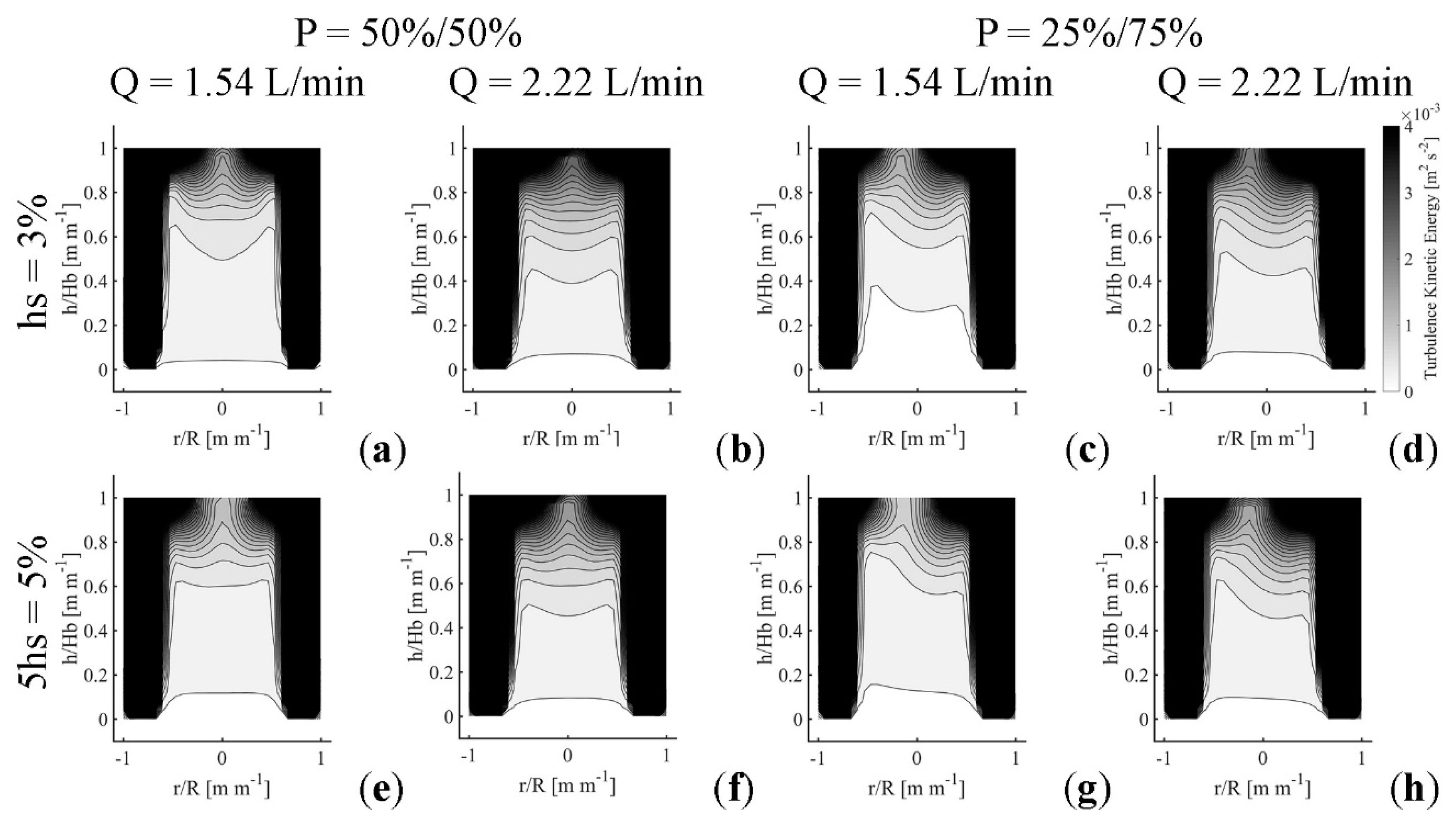
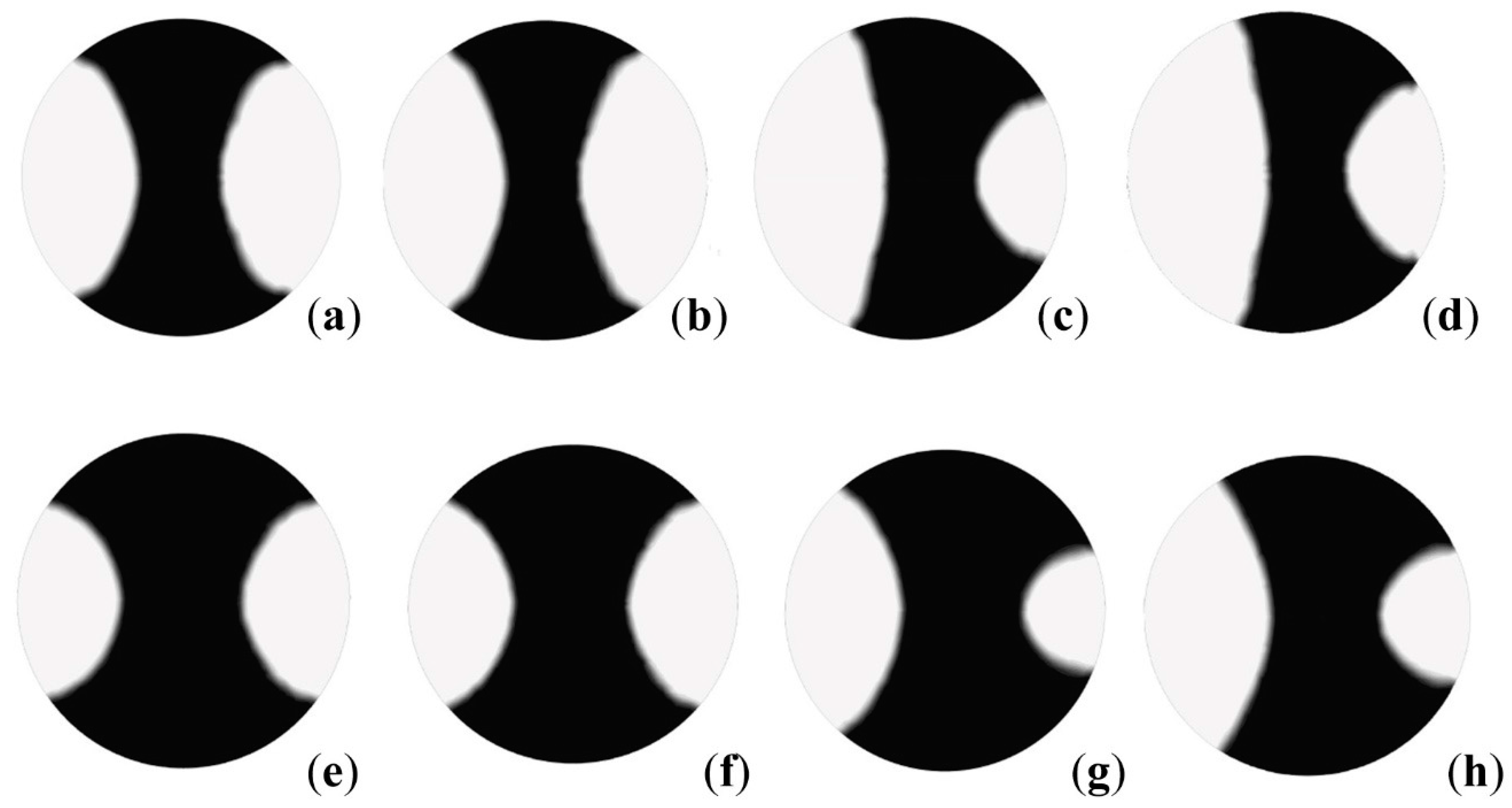
19] studied mixing time and slag eye area fitted with dual plugs as a function of operating variables, namely, gas flow rate, radial nozzle position, separation angle between nozzles and partitioning flow rate. They suggested that if mixing time is the parameter of primary interest then nozzle configuration with equal flow partitioning (50%:50%) between the nozzles should suffice for both low and high gas flow rates, whereas if slag eye is the parameter of primary interest then a configuration with non-equal flow partitioning (25%:75%) between the nozzles should be preferred. Villela-Aguilar et al. [20] performed a multiphase numerical simulation to analyze the effects of the gas flow rate, radial position and angle between plugs and differentiated flows in two plugs on the mixing time in a secondary refining ladle. They found that the angle of separation between the plugs is the most relevant variable to reduce mixing time. They also found that it is possible to reduce the mixing time by using a good differentiated configuration in both gas flow and location of the porous plugs. According to a review by Liu et al. [17], there is still room for further improvement of the numerical model regarding the representation of the turbulence and the slag–steel interactions. One of the least studied variables, in the case of dual gas injection points, is the effect of the use of different gas flow rates in each plug (i.e., a gas blowing ratio different from 50%:50%).
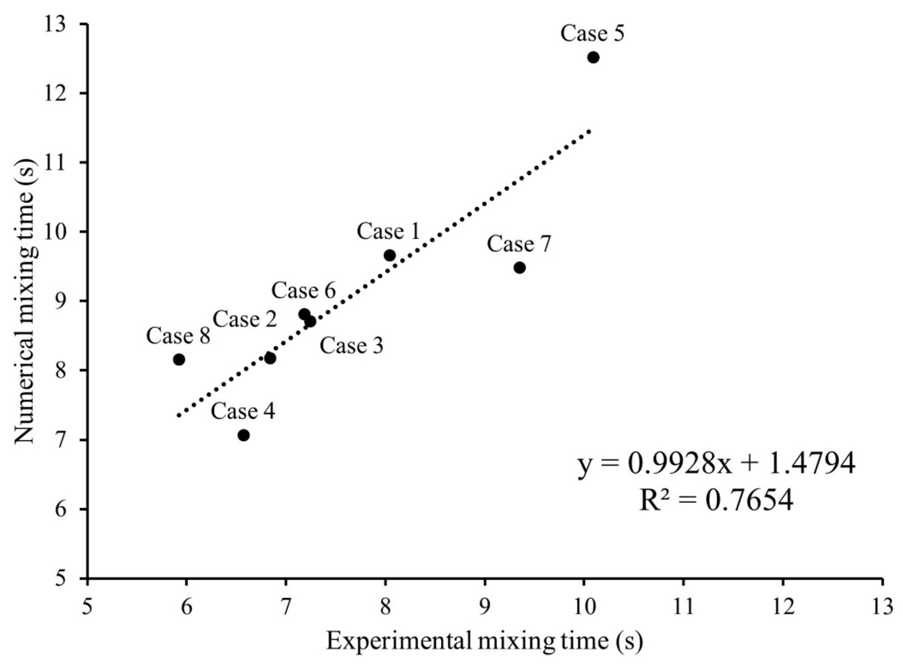
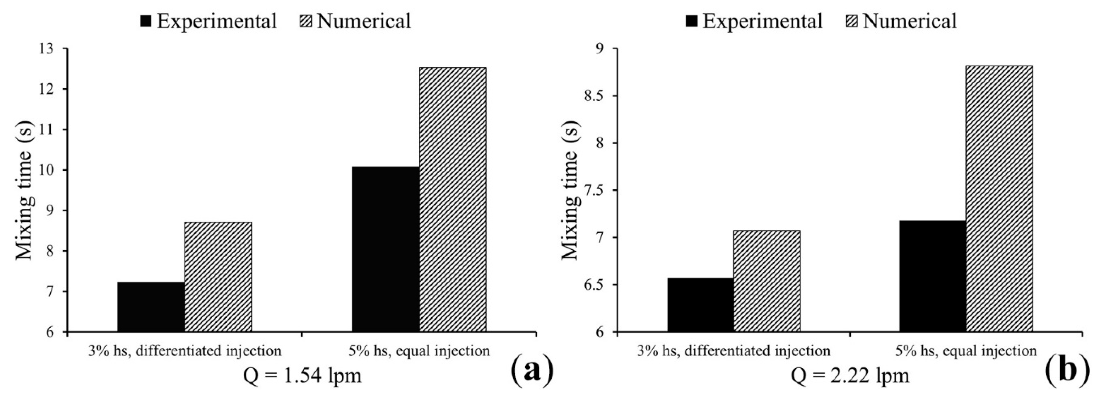
In the present study, the effect of gas injection in equal (50%:50%) and differentiated (75%:25%) flows, along with the gas flow rate and slag thickness, on mixing time and slag eye were studied using a numerical model of a ladle and were compared with previously-obtained experimental data based on PIV measurements of the hydrodynamics and PLIF measurements of mixing time for model validation. This study aims to improve the mixing time in a secondary refining ladle and to identify a balanced compromise between mixing time and slag eye, while improving numerical modeling practices using experimental data on differentiated dual gas injection modes in ladles.

2. Methodology: Numerical Model Development

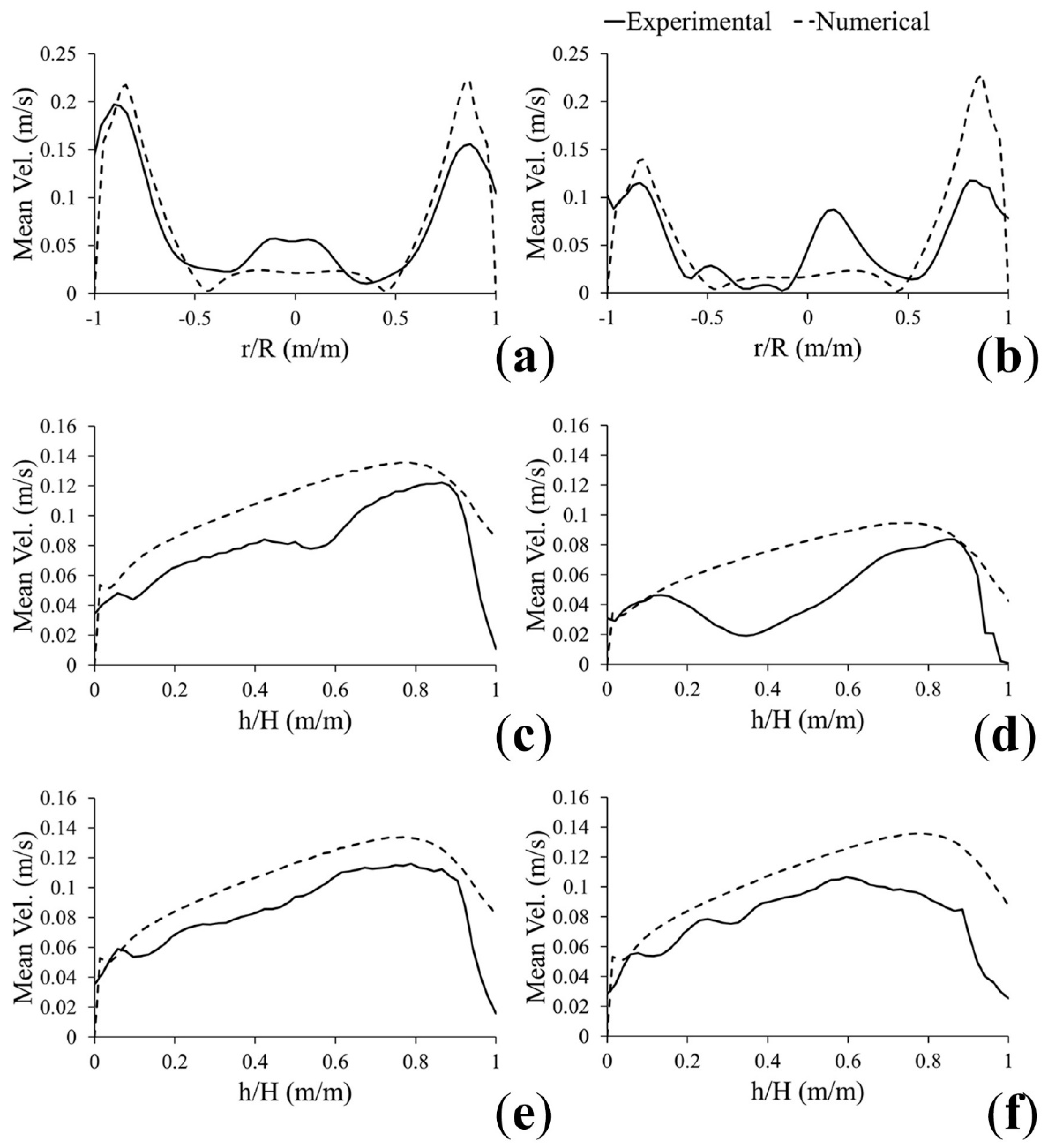
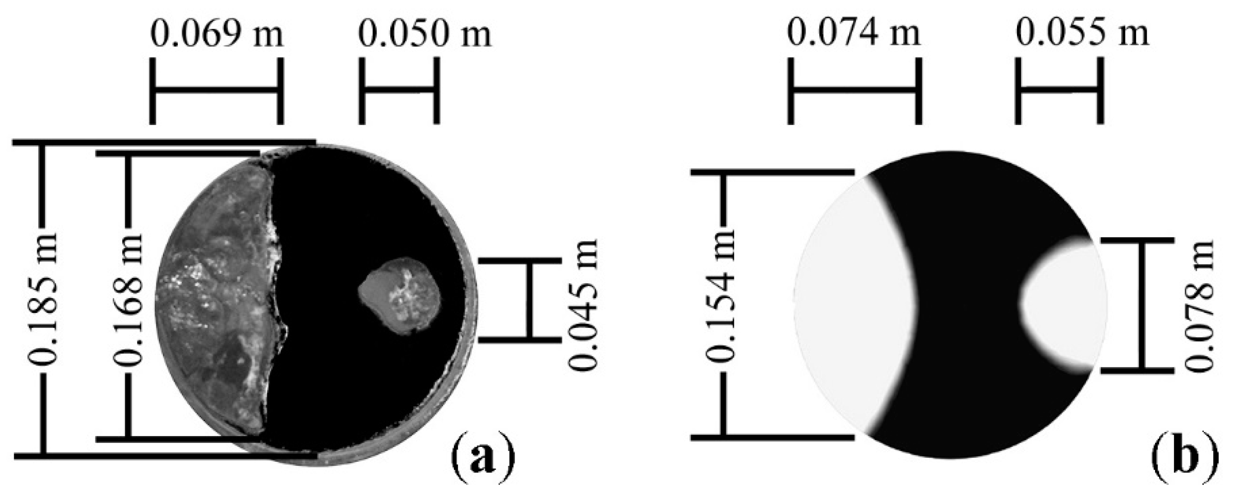
A Eulerian multi-phase mathematical model simulating the physical model described in this study was developed under the following assumptions: (i) steady state, (ii) a symmetry plane is considered for the dual gas injection system and thus only half of the ladle is solved; (iii) Newtonian and incompressible fluids for both liquids and gas phases; (iv) isothermal flow and (v) constant bubble diameter of 0.01 m. The latter is certainly an oversimplification, by neglecting bubble disintegration and coalescence phenomena under real dynamic bubble size distributions. However, using the Eulerian model most regions of the ladle are fairly well predicted, as presented in Section 3.1, both in turbulence and velocity magnitude, except for the water-oil-bubble open eye regions. Governing equations for the 3D Eulerian-Eulerian multi-phase algorithm include mass conservation equation, Navier–Stokes equations and the k- ε realizable turbulence model for the water phase.
The volume of the q-phase, V q , is given by the volume integral:
V q = V q d V
where q is the volume fraction of phase q, and the sum of volume fractions must be equal to one according to:
q = 1 n q = 1
The continuity equation for each q-phase is:
· ( q ρ q v q ) = 0
where ρ q and v q are the density and velocity vector of the q-phase, respectively.
The momentum conservation equation for the q-phase is:
· ( q ρ q v q v q ) = q P + · ( q μ e f , q ( v q + ( v q ) T ) ) + q ρ q g + F T
For the water phase:
μ e f , l = μ l a m , l + μ t , l
For other phases:
μ e f , q = μ l a m , q
where P , μ e f , q , g are the pressure, effective viscosity of the q-phase and the gravity acceleration, respectively. The effective viscosity for the water phase is the sum of the molecular viscosity ( μ l a m , l ) and the turbulent viscosity ( μ t , l ) defined by the turbulence model employed. For the other phases μ l a m , q is only the laminar viscosity of every fluid, and the subscripts l and l a m stand for water and laminar, respectively. The term F T is the contribution of all interphase forces. The only force considered is the drag force, and the virtual mass, lift and turbulent dispersion forces are neglected.
In this study, a sensitivity analysis was performed to choose the best turbulence model that predicts correctly the turbulence measured in the ladle. From all the models tested, the best option is the realizable k - ε turbulence model [21]. This model solves two additional conservation equations applicable only to the water liquid phase, one of these equations being the conservation of turbulent kinetic energy, k :
· ( α l ρ l k v l ) = · ( α l ( μ l a m , l + μ t , l σ k ) k ) + α l G k , l + α l G b α l ρ l ε + α l ρ l π k , l
The conservation equation for the dissipation of the turbulent kinetic energy, ε :
· ( α l ρ l ε v l ) = · ( α l ( μ l a m , l + μ t , l σ ε ) ε ) + α l C 1 ( ε k G b C 3 ) α l ρ l C 2 ε 2 k + ε μ l a m , l ρ l + α l ρ l π ε , l
C 1 , C 2 , C 3 , σ k and σ ε are constants of the model, with values of 1.44, 1.92, 1.3, 1.0 and 1.2 respectively. G k is the production of turbulent kinetic energy due to the mean velocity gradients of the water phase and G b is the additional turbulent kinetic energy produced by the bubbles. π k , l and π ε , l are the turbulent interaction terms defined by Troshko-Hassan [22] as:
π k , l = C k e p = 1 m K g l | v g v l | 2
π ε , l = C t d 3 C A | v g v l | 2 d g π k , l
where C k e and C t d are model constants with values of 0.75 and 0.45, respectively. K g l is the covariance of the velocities of the continuous phase l and the disperse phase g . d g is the bubble diameter; the velocity difference between the gas and liquid phase, ( v g v l ) , is defined as the relative velocity, v r e l ; whereas C A is the drag coefficient determined through a sensitivity analysis (not mentioned in this study) performed that revealed the best option was the well-known symmetric model:
C A = { 24 ( 1 + 0.15 R e 0.687 ) R e   R e 1000 0.44   R e > 1000
where R e is the Reynolds number.
The interphase forces, F T are limited to the drag force, F A as follows:
F T = F A = 3 α g α l ρ l C A 4 d g ( v g v l )
Finally, to compute mixing time in the water phase l , a single conservation equation for a tracer chemical species i is solved in transient mode with initial conditions of zero concentration of solute everywhere except for the pulsed tracer injected at the free surface above the plume of high flow, as follows:
t ( ρ l w i , l ) + · ( ρ l u l w i , l ) = · ( ρ l D i , l + μ t , l S c t ) w i , l
The geometry of the water (physical) model that was used in PIV experiments is made in 3D using ANSYS Design Modeler 19.0 (Ansys Inc., Canonsburg, PA, USA) for the numerical model. The diameter and height of the cylindrical ladle are 0.185 m and 0.214 m (0.17 m liquid level), respectively, similar to that of the physical model [15] that corresponds to a 1:17 scale ratio of an industrial-size ladle of 200-ton capacity. 
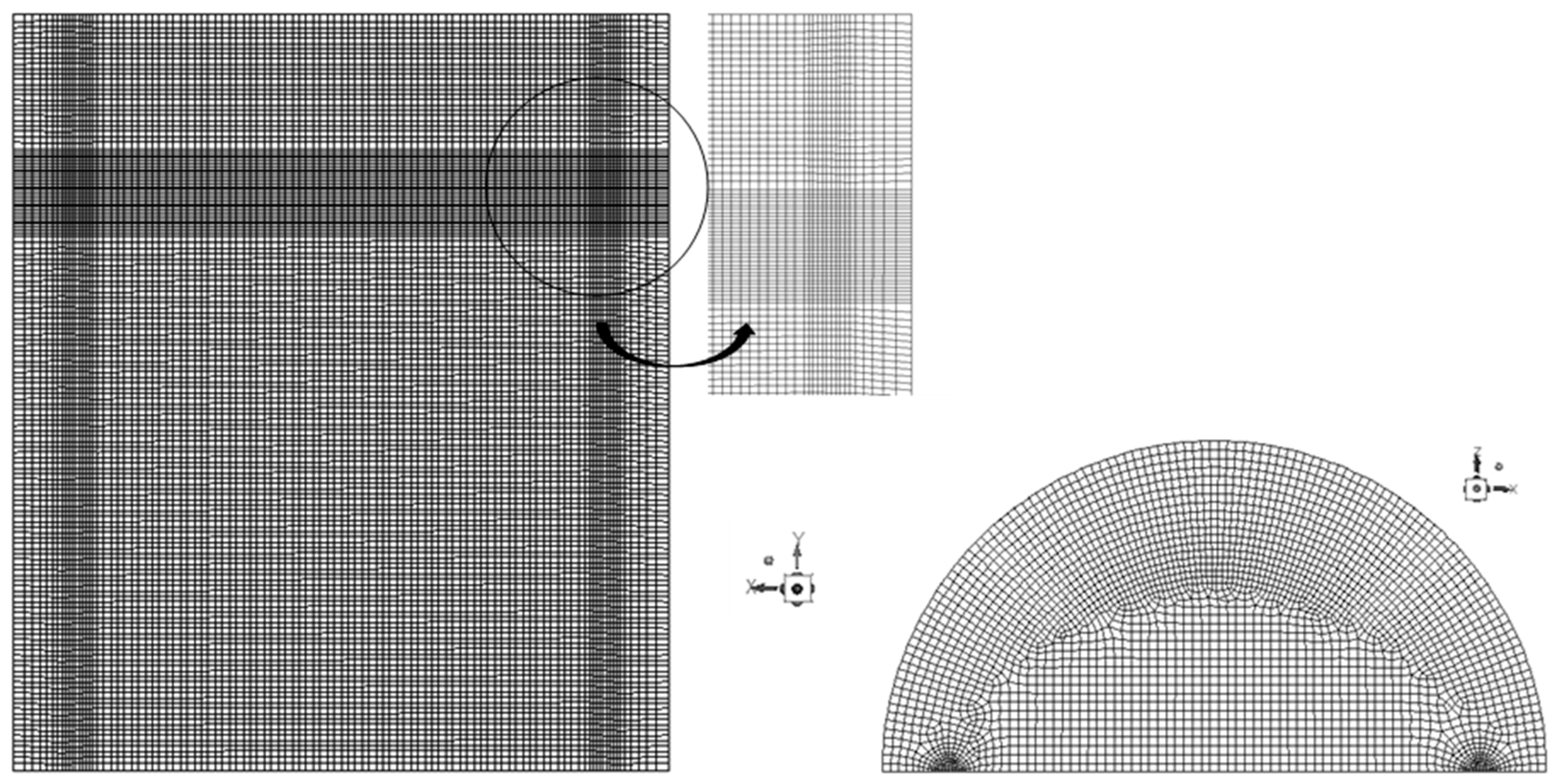
Figure 1 shows an illustration of the mesh built with approximately 350,000 elements with average orthogonality, skewness and aspect ratios of 0.98, 0.1 and 1.99, respectively. The choice of the mesh elements was based on a sensitivity analysis using approximately 200,000 and 500,000 mesh elements.
Non-slip boundary conditions at the bottom and lateral walls have been used, whereas the standard wall functions have been used to connect the turbulent core of the fluid with the laminar flow near the walls. The gas injection inlets at the nozzle positions and an open boundary to the atmosphere at the top of the system allow the outflow of the gas phase. The complete set of boundary conditions can be found in Table 1.
The system of partial differential equations was numerically solved and the solution in pseudo-transient mode was considered to be converged when the residuals of all conservation equations were below 1 × 10⁻³. Approximately 1200 iterations were required to get the convergence in around 36 h of CPU time in a computer with 8 MB in RAM with an Intel Core® i7-3770 processor of 3.4 GHZ. Table 2 lists all the numerical simulations performed in this study which is based on a full factorial experimental design at two levels with the three variables, namely, gas flow rate, dual gas injection ratio and (slag) oil thickness, as mentioned in Jardón-Pérez et al. [15].

3. Results and Discussion

3.1. Model Validation

Figure 2 shows the flow patterns obtained through the PIV technique reported in Jardón-Pérez et al. [15] at different operating conditions listed in Table 2, whereas Figure 3 shows the flow patterns obtained with the numerical model presented in this study. As seen in these figures, a reasonable agreement is observed between experimental and numerical results for all the cases. For equal (50%:50%) dual gas injection, two symmetric toroids are formed at each side of the plume, whereas for unequal (25%:75%) injection, symmetry vanishes and the high flow rate circulation expands at the expense of the low flow rate circulation loop. An increase in the gas flow rate increases the expansion of the plume in general, and for unequal injection further expands the high-flow rate circulation loop. The increment in (slag) oil thickness mitigates the inertia of the plumes, reducing the velocities of the liquid, and diminishes the loop expansions. An increase in (slag) oil thickness lowers the velocity of the liquid in the vicinity of the oil layer at the top of the ladle. In general, the experimental results were predicted successfully with the model, but some differences were also perceived. The numerical predictions using CFD do not account for the expansion of the bigger loop for unequal injection as occurs in PIV-measured flow patterns. As an illustration, Figure 4 shows measured (a) and calculated (b) streamlines obtained for experiment b (see Table 2) under equal dual gas injection, showing good agreement between both predicted and measured streamlines; however, under unequal dual gas injection for experiment g (see Table 2), calculated (d) streamlines do not capture the expansion of the strong plume and the contraction of the small loop as seen in the measured (c) streamlines. In general, the magnitudes of the liquid velocity were slightly underestimated. Mean value was overestimated (see Table 3), but the distribution is quite different, especially in differentiated injection, since the model does not accurately predict the interaction of the plumes. In the case of differentiated dual gas injection, the interaction between the recirculation loops was not observed. This is probably due to the drag effect, which was not successfully implemented, and represents a challenging issue in numerical modeling, from the hydrodynamic point of view, of the more complex multiple differentiated dual gas injections, compared to the traditional equal dual gas injection. Despite the differences, the numerical model of the ladle furnace in steady state showed good results, with a reasonable agreement with the experimentally measured liquid flow patterns reported in Jardón-Pérez et al. [15]. A more quantitative validation is shown in Figure 5 by comparing experimental (continuous line) and numerical (dotted line) mean velocity radial profiles at h/H = 0.8 for experiments b (a) and g (b); axial profiles at r/R = −0.75 for experiments b (c) and g (d); and axial profiles at r/R = 0.75, for experiments b (e) and g (f). In all these cases, a good agreement between prediction and measurement is achieved, with, in general, the numerical velocity profiles slightly over-predicting the measured results, but with the simulations capturing the measured liquid motion in the plumes.

3.2. Turbulence Modeling

Figure 6 shows the simulated profiles of turbulent kinetic energy (k) at the same operating conditions of Figure 2 (see Table 2 for the sequence of the experiments). A reasonable agreement can be seen in Table 4 between the experimental and numerical results of turbulence, showing that the k-ε realizable turbulence model was an appropriate choice to represent turbulence in the three-phase fluid flow system implemented in this study. Due to the turbulence promoted by the bubbles, high turbulence zones corresponding to the two plume zones were observed. By increasing the gas flow rate (Figure 6b,d) the values of turbulent kinetic energy k in the circulation loops increase. A thicker slag reduces turbulence and the interaction between the loops. Although the magnitudes of the turbulent kinetic energy k in the plane overestimated the experimental results in almost all cases (in comparison with Figure 4 of Jardón-Pérez et al. [15]), the above-mentioned main effects of the three variables on k were successfully predicted with the numerical model. However, some features were not captured by the model, such as the drag effect (comparing Figure 2h with Figure 3h), where the smaller plume zone was not attracted to the center due to the influence of the loop.

3.3. Slag Eye Modeling

Tang et al. [14] compared the change in slag eye area between equal and differentiated flows at various gas injection parameters, including the angle between the dual plugs from 45° to 180° and its radial position from r/R = 0.5 to r/R = 0.7 and the gas flow rate. They found that in most cases the proportion of slag eye in the differentiated flow system is smaller than that in the equal flow system. Their results show that the proportion of slag eye in differentiated flow first decreases and then increases with the increasing relative angle of plugs at the same flowrate, and the exposed areas of the slag eyes of the two modes generally decrease with plug position from 0.55R to 0.70R, apparently due to the obstacle of the ladle wall and its absorption of the stirring energy. The slag eye is the smallest at 0.7R–90° and 0.7R–135°. Conejo et al. [19] measured the change in the slag eye area between equal and differentiated flows for two nozzle radial positions (0.7R/0.7R and 0.7R/0.5R) and two angles (45° and 90°). Their results show that the use of differentiated flow increases the area of slag eye for an angle of 45° and equal plug positions, whereas there is a decrease in the eye when using unequal plug positions and an angle between plugs of 90°. From these results, it can be seen that the change in slag eye becomes rather complex in the presence of multiple variables.
Figure 7 presents the time-averaged predicted slag eye of the eight experiments (see Table 2) using the developed numerical model. The effect of the three variables, namely, gas flow rate, dual gas injection ratio and (slag) oil thickness on the size of the slag eye was predicted. As seen in the experiment, an increase in gas flow rate increases the extent of slag eye area in all cases, whereas the opposite effect is obtained with an increase of (slag) oil thickness. A good agreement between the experimental results (see Figure 5 of Jardón-Pérez et al. [15]) and the numerical results can be seen in Table 5, with slag eye area as a percentage of the total surface. Again, the drag effect generated with a differentiated gas injection was not captured completely by the model, i.e., the smaller slag eye is not attracted to the center as observed in the experimental results, but the shapes of the slag eye were correctly predicted. For example, for the case with 5% (slag) oil thickness and differentiated 2.22 L/min gas flow rate, presented in Figure 8, the numerical size of the big eye is slightly under-predicted, whereas the small eye is over-predicted, when compared against the measured eyes. As mentioned earlier, the velocity field near the water–oil (steel–slag) interface and the slag eye size features are not properly captured by the numerical model, which opens an opportunity for improvement of the physical description of the interaction between the two phases through the modification of forces such as drag and surface tension.

3.4. Mixing Time Modeling

Mixing phenomena in metallurgical steel ladles by bottom gas injection involve three phases, namely, liquid molten steel, liquid slag and gaseous argon. Mixing time is the time needed for an established constant flow field to disperse an injected non-reactive tracer until the required mixing criterion is achieved. This criterion is generally set to 95%, although 99% and 99.5% [23,24] can be used as well. Typically, the mixing efficiency of a ladle is qualified as the mixing time ( τ m ) and is an important indicator for the hydrodynamic performance to quantify the degree of agitation, which influences secondary refining treatment in a ladle through desulphurization. Lou and Zhu [25] modeled desulfurization and inclusion removal in a ladle with multiple nozzle configurations. They concluded that dual nozzle configurations have a higher desulfurization rate than single nozzle configurations for the same flow rate. Zhu et al. [26] investigated the mixing phenomena in argon-stirred ladles with six types of tuyere arrangement. They concluded that mixing time is greatly influenced by the position of the tracer, and that mixing time decreases with increasing gas flow rate, although the effect is not so remarkable. Haiyan et al. [13] studied the effect of gas flow rate on the mixing phenomenon in a bottom-stirring ladle with dual plugs. They found that compared with the same flowrate for the two plugs, the mixing time is lower with different flow rates when the plug positions are located at 0.64R. This is mainly due to the strong gas plume, which produces a larger circulation flow to stir the ladle. A weaker plume forms a smaller one, which weakens the interference and collision from the two plumes, thus reducing the mixing time. Recently, Ramasetti et al. [27] calculated the mixing time of tracer addition into the metal bath of a ladle, which decreased when the argon flow rate was increased.
Nunes et al. [28] were among the earliest to use a dye tracer to determine the mixing time in a ladle, thus eliminating the dependence on the monitoring position. For the measurement of mixing time, techniques such as using a pH meter or conductivity meter are the most common, although more recently dye tracers and laser-induced fluorescence (LIF) have been used. To measure the time needed to reach a stable state, usually a criterion of ± 5% of variation of property is used, which can be measured by pH in a pH meter, conductivity in a conductivity meter, and tracer concentration and luminescence in LIF. In the experimental study of Jardón-Pérez et al. [15], mixing time in a gas-stirred ladle was measured by means of the novel technique of planar laser-induced fluorescence (PLIF) that uses Rhodamine 6G as a tracer. PLIF determinations were performed at two different planes and pH probe determinations were performed at two different locations. The results were then compared, which showed not only the accuracy of the PLIF method, but also that it is less sensitive to the location of the measurement than the pH probe method. A detailed explanation of the technique can be found in Jardón-Pérez et al. [29]. Ascanio [30] does not recommend the technique for highly aerated flows, because the presence of bubbles complicates the calibration and the measurement of the obtained concentration contour.
From the experimental study of Jardón-Pérez et al. [15], it was found that all cases gave smaller mixing times with the same conditions of (slag) oil thickness and dual gas injection ratio. The increase in the thickness gave slightly higher mixing times. The numerical model of the mixing time presented in this study gave very similar results to the experimental mixing time for both 50%:50% equal flow and 25%:75% dual differentiated flow. As with the experimental study, the effect of a 25%:75% dual injection ratio is slightly less significant with conditions of high gas flow rate (2.22 L/min) as compared with conditions of low gas flow rate (1.54 L/min) for 3% (slag) oil thickness than with 5% (slag) oil thickness (see Table 6). The deviation from the experimental mixing time was found to be the greatest for 25%:75% dual differentiated flow at a high gas flow rate (2.22 L/min), whereasthe deviation was found to be the lowest for 25%:75% dual differentiated flow at low gas flow rate (1.54 L/min) both at 5% oil thickness. The difference between experimental and predicted mixing times can be explained by comparing the experimental (Figure 2) and numerical (Figure 3) flow patterns. As can be seen, the area of the low-velocity zone with dual injection is higher for the numerical model than the physical model, mainly due to the difficulty of simulating the interaction between both the gas plumes, especially when a differentiated injection is used. This is because the interaction between the low-injection and the high-injection plumes (see Figure 3c,d,g,h) shows a large deformation in both plume structures due to the drag force that the high-injection plume exerts on the low-injection plume.
Figure 9 shows the trend in the model predictions and the experimental results reported in Jardón-Pérez et al. [15] based on all the cases implemented in this study. In this Figure, it is seen that the model is able to capture the more important issues regarding the behavior of the system under different experimental conditions. Considering that differences between predicted and experimental measurements increase for differentiated gas injection and high slag thickness (Cases 7 and 8 in Figure 9 and Table 2), the results suggest that these are places in which to seek improvements in the numerical model, especially in high slag thickness. This is probably because with a higher slag thickness the influence of slag emulsification on mixing time becomes prominent, since the numerical model does not consider the emulsified droplets. This is also shown clearly in Figure 10, which depicts the difference in the model prediction compared with the experimental results reported in Jardón-Pérez et al. [15] for the cases of low gas flow rate (Figure 10a) and high gas flow rate (Figure 10b), thus exploring the ability of the numerical model to capture the two limit cases analyzed in this study.
In both figures, the best match is obtained for the case of low gas flow rate and low slag thickness. At a high flow rate, the differences between experimental and predicted results increase for all cases (see Table 6) and these differences are bigger for differentiated gas injection, independently of the gas flow rates. The results suggest that modeling efforts must be focused on the improvement of the turbulence model, as well as finding approaches to simulate the effect of the slag layer (mainly the slag emulsification) on the flow dynamics of the stirred melt and to simulate changes in the flow plume linked to the change in the mode of gas injection.
However, even if numerical values of both slag eye area and mixing time show differences between numerical and experimental values (see Table 5 and Table 6), the effect of the studied variables is correctly predicted by the mathematical model, i.e., an increase in gas flow rate causes an increase in the exposed area and a decrease in the mixing time, an increase in slag height causes a decrease in the slag eye area and an increment in the mixing time, and finally, the use of differentiated gas injection causes a slight increment in the exposed area but also a decrement in the mixing time compared with equal injection. Therefore, the CFD numerical model could be used to study the main effects of operation variables on both mixing time and slag eye area.

4. Conclusions

In the numerical study of the effect of dual gas injection using equal (50%:50%) and differentiated (75%:25%) flows and variable (slag) oil thickness compared with the experimental results obtained previously, the following conclusions can be made:
  • The numerical model using CFD predicts the hydrodynamic behavior of the ladle well, in comparison with the physical model. Turbulent kinetic energy is adequately and qualitatively predicted, although it is somewhat overestimated. It can be said that the model qualitatively predicts the influence of the gas flow, the distribution of the flows and the level of slag on the distribution of velocities and turbulence.
  • The predicted slag eye shows a good agreement with the experimental results with slag eye area as a percentage of the total surface. However, due to the interphase interaction, the slag eye from differentiated gas injection is not captured completely by the model.
  • The numerical model does not fully predict the effect of differentiated gas injection, since the drag model used does not exactly simulate the interaction between both recirculation zones, hence predicting a smaller area of low-velocity zones.
  • There is a deviation in predicted mixing time from experimental mixing time for both equal and differentiated gas injection, which becomes significant at a high gas flow rate and a high slag thickness.
The anomaly in the observations is attributed to the insufficient capture of the hydrodynamic behavior near the water–oil (steel–slag) interface, probably caused by the emulsification of slag, which might also influence changes in the gas plumes, linked to the change in the mode of gas injection. This is coupled with the difficulty of accurately predicting the complex interaction between the gas plumes, especially in differentiated injection, which causes a variation in the predicted values of mixing time and slag eye area, although the effect of the variables (gas flow rate, slag height and injection mode) can be studied with an in-depth understanding of the mathematical model presented.

Author Contributions

Conceptualization, M.A.R.-A. and A.D.; methodology, L.E.J.-P.; software, L.E.J.-P. and A.D.; validation, L.E.J.-P. and C.G.-R.; formal analysis, C.G.-R.; investigation, L.E.J.-P. and C.G.-R.; resources, L.E.J.-P.; writing—original draft preparation, L.E.J.-P.; writing—review and editing, A.D. and C.G.-R.; supervision, A.D.; funding acquisition, M.A.R.-A. All authors have read and agreed to the published version of the manuscript.

Funding

This research was funded by [DGAPA UNAM] grant number [PAPIIT IN115619] and L.E.J.-P. received PhD scholarship by [CONACYT] grant number [CVU 624968].

Conflicts of Interest

The authors declare no conflict of interest.

References

  1. Ghosh, A. Secondary Steelmaking: Principles and Applications; CRC Press LLC: Boca Raton, FL, USA, 2001. [Google Scholar]
  2. Du, S. Improving process design in steelmaking. In Fundamentals of Metallurgy; Elsevier Inc.: Amsterdam, The Netherlands, 2005; pp. 369–398. [Google Scholar]
  3. Mazumdar, D.; Evans, J.W. Macroscopic Models for Gas Stirred Ladles. ISIJ Int. 2004, 44, 447–461. [Google Scholar] [CrossRef] [Green Version]
  4. Amaro-Villeda, A.M.; Ramírez-Argáez, M.A.; Conejo, A.N. Effect of Slag Properties on Mixing Phenomena in Gas-stirred Ladles by Physical Modeling. ISIJ Int. 2014, 54, 1–8. [Google Scholar] [CrossRef] [Green Version]
  5. Hoang, Q.N.; Ramírez-Argáez, M.A.; Conejo, A.N.; Blanpain, B.; Dutta, A. Numerical Modeling of Liquid–Liquid Mass Transfer and the Influence of Mixing in Gas-Stirred Ladles. JOM 2018, 70, 2109–2118. [Google Scholar] [CrossRef]
  6. Asai, S.; Okamoto, T.; He, J.-C.; Muchi, I. Mixing Time of Refining Vessels Stirred by Gas Injection. Trans. Iron Steel Inst. Jpn. 1983, 23, 43–50. [Google Scholar] [CrossRef] [Green Version]
  7. Sano, M.; Mori, K. Fluid flow and mixing characteristics in a gas-stirred molten metal bath. Trans. Iron Steel Inst. Jpn. 1983, 23, 169–175. [Google Scholar] [CrossRef]
  8. Joo, S.; Guthrie, R.I.L. Modeling flows and mixing in steelmaking ladles designed for single- and dual-plug bubbling operations. MTB 1992, 23, 765–778. [Google Scholar] [CrossRef]
  9. Krishnapisharody, K.; Irons, G.A. An Analysis of Recirculatory Flow in Gas-Stirred Ladles. Steel Res. Int. 2010, 81, 880–885. [Google Scholar] [CrossRef]
  10. Khajavi, L.T.; Barati, M. Liquid Mixing in Thick-Slag-Covered Metallurgical Baths—Blending of Bath. Met. Mater. Trans. B 2010, 41, 86–93. [Google Scholar] [CrossRef]
  11. Chattopadhyay, K.; Sengupta, A.; Ajmani, S.K.; Lenka, S.N.; Singh, V. Optimisation of dual purging location for better mixing in ladle: A water model study. Ironmak. Steelmak. 2009, 36, 537–542. [Google Scholar] [CrossRef]
  12. Liu, H.; Qi, Z.; Xu, M. Numerical Simulation of Fluid Flow and Interfacial Behavior in Three-phase Argon-Stirred Ladles with One Plug and Dual Plugs. Steel Res. Int. 2011, 82, 440–458. [Google Scholar] [CrossRef]
  13. Haiyan, T.; Xiaochen, G.; Guanghui, W.; Yong, W. Effect of Gas Blown Modes on Mixing Phenomena in a Bottom Stirring Ladle with Dual Plugs. ISIJ Int. 2016, 56, 2161–2170. [Google Scholar] [CrossRef] [Green Version]
  14. Tang, H.; Liu, J.; Zhang, S.; Guo, X.; Zhang, J. A novel dual plugs gas blowing mode for efficient ladle metallurgy. Ironmak. Steelmak. 2019, 46, 405–415. [Google Scholar] [CrossRef]
  15. Jardón-Pérez, L.E.; González-Morales, D.R.; Trápaga, G.; González-Rivera, C.; Ramírez-Argáez, M.A. Effect of Differentiated Injection Ratio, Gas Flow Rate, and Slag Thickness on Mixing Time and Open Eye Area in Gas-Stirred Ladle Assisted by Physical Modeling. Metals 2019, 9, 555. [Google Scholar] [CrossRef] [Green Version]
  16. Mazumdar, D.; Dhandapani, P.; Sarvanakumar, R. Modeling and Optimisation of Gas Stirred Ladle Systems. ISIJ Int. 2017, 57, 286–295. [Google Scholar] [CrossRef] [Green Version]
  17. Liu, Y.; Ersson, M.; Liu, H.; Jönsson, P.G.; Gan, Y. A Review of Physical and Numerical Approaches for the Study of Gas Stirring in Ladle Metallurgy. Met. Mater. Trans. B 2018, 50, 555–577. [Google Scholar] [CrossRef] [Green Version]
  18. Li, B.; Yin, H.; Zhou, C.Q.; Tsukihashi, F. Modeling of Three-phase Flows and Behavior of Slag/Steel Interface in an Argon Gas Stirred Ladle. ISIJ Int. 2008, 48, 1704–1711. [Google Scholar] [CrossRef] [Green Version]
  19. Conejo, A.N.; Mishra, R.; Mazumdar, D. Effects of Nozzle Radial Position, Separation Angle, and Gas Flow Partitioning on the Mixing, Eye Area, and Wall Shear Stress in Ladles Fitted with Dual Plugs. Met. Mater. Trans. B 2019, 50, 1490–1502. [Google Scholar] [CrossRef]
  20. Villela-Aguilar, J.D.J.; Ramos-Banderas, J.Á.; Hernández-Bocanegra, C.A.; Urióstegui-Hernández, A.; Solorio-Díaz, G. Optimization of the Mixing Time Using Asymmetrical Arrays in Both Gas Flow and Injection Positions in a Dual-plug Ladle. ISIJ Int. 2020, 60, 1172–1178. [Google Scholar] [CrossRef] [Green Version]
  21. Shih, T.-H.; Liou, W.W.; Shabbir, A.; Yang, Z.; Zhu, J. A new k-ϵ eddy viscosity model for high reynolds number turbulent flows. Comput. Fluids 1995, 24, 227–238. [Google Scholar] [CrossRef]
  22. Troshko, A.A.; Hassan, Y.A. A two-equation turbulence model of turbulent bubbly flows. Int. J. Multiph. Flow 2001, 27, 1965–2000. [Google Scholar] [CrossRef]
  23. Krishnakumar, K.; Ballal, N.B.; Sinha, P.K.; Sardar, M.K.; Jha, K.N. Water Model Experiments on Mixing Phenomena in a VOD Ladle. ISIJ Int. 1999, 39, 419–425. [Google Scholar] [CrossRef]
  24. González-Bernal, R.; Solorio-Diaz, G.; Ramos-Banderas, A.; Torres-Alonso, E.; Hernández-Bocanegra, C.A.; Zenit, R. Effect of the Fluid-Dynamic Structure on the Mixing Time of a Ladle Furnace. Steel Res. Int. 2018, 89, 1700281. [Google Scholar] [CrossRef]
  25. Lou, W.; Zhu, M. Numerical Simulation of Slag-metal Reactions and Desulfurization Efficiency in Gas-stirred Ladles with Different Thermodynamics and Kinetics. ISIJ Int. 2015, 55, 961–969. [Google Scholar] [CrossRef] [Green Version]
  26. Zhu, M.-Y.; Inomoto, T.; Sawada, I.; Hsiao, T.-C. Fluid Flow and Mixing Phenomena in the Ladle Stirred by Argon through Multi-Tuyere. ISIJ Int. 1995, 35, 472–479. [Google Scholar] [CrossRef]
  27. Ramasetti, E.; Visuri, V.-V.; Sulasalmi, P.; Fabritius, T.; Saatio, T.; Li, M.; Shao, L. Numerical Modeling of Open-Eye Formation and Mixing Time in Argon Stirred Industrial Ladle. Metals 2019, 9, 829. [Google Scholar] [CrossRef] [Green Version]
  28. Nunes, R.P.; Pereira, J.A.M.; Vilela, A.C.F.; Laan, F.T.V. Visualisation and analysis of the fluid flow structure inside an elliptical steelmaking ladle through image processing techniques. J. Eng. Sci. Technol. 2007, 2, 139–150. [Google Scholar]
  29. Jardón-Pérez, L.E.; Amaro-Villeda, A.; González-Rivera, C.; Trápaga, G.; Conejo, A.N.; Ramírez-Argáez, M.A. Introducing the Planar Laser-Induced Fluorescence Technique (PLIF) to Measure Mixing Time in Gas-Stirred Ladles. Met. Mater. Trans. B 2019, 50, 2121–2133. [Google Scholar] [CrossRef]
  30. Ascanio, G. Mixing time in stirred vessels: A review of experimental techniques. Chin. J. Chem. Eng. 2015, 23, 1065–1076. [Google Scholar] [CrossRef]
Figure 1. Computational domain of the ladle used for the numerical simulations presented in this study. The two vertical sections indicating the gas injection inlets and the top horizontal section indicating the slag layer are comparatively denser than the remaining mesh domain. The inset shows the mesh density for the slag zone which is different from the melt zone. The top portion of the mesh (half along the symmetry plane) is shown separately.
Processes 08 00917 g001
Figure 2. Flow patterns of the eight case studies obtained with the experimental model (particle image velocimetry (PIV) technique) in the longitudinal plane. (a) through (h) are the experiments described in Table 2.
Processes 08 00917 g002
Figure 3. Flow patterns of the eight case studies obtained with the numerical model and shown along the same longitudinal plane. (a) through (h) are the experiments described in Table 2. The cases presented in this study are in the same order as in the experimental study of Jardón-Pérez et al. [15].
Processes 08 00917 g003
Figure 4. Streamlines obtained for experiment b (Table 2), measured (a) and calculated (b); and for experiment g (Table 2), measured (c) and calculated (d).
Processes 08 00917 g004
Figure 5. Comparison of experimental (continuous line) and numerical (dotted line) mean velocity radial profiles at h/H = 0.8 for experiments b (a) and g (b); axial profiles at r/R = −0.75 for experiments b (c) and g (d); and axial profiles at r/R = 0.75 for experiments b (e) and g (f).
Processes 08 00917 g005
Figure 6. Contours of turbulent kinetic energy (k) of the eight case studies obtained with the numerical model and shown along the same longitudinal plane. (a) through (h) are the experiments described in Table 2. The cases presented in this study are in the same order as in the experimental study of Jardón-Pérez et al. [15].
Processes 08 00917 g006
Figure 7. Time-averaged prediction of slag eyes at different operating conditions obtained with the numerical model. (a) through (h) are the experiments described in Table 2. The cases presented in this study are in the same order as in the experimental study of Jardón-Pérez et al. [15].
Processes 08 00917 g007
Figure 8. Comparison of the time-averaged photograph of the slag eye obtained with the (a) experimental model (operating condition of differentiated dual gas injection with 5% (slag) oil thickness and 2.22 L/min gas flow rate) and the corresponding time-averaged (b) numerical model prediction. Dimensions of measured and predicted open slag eyes are also indicated.
Processes 08 00917 g008
Figure 9. Comparison between the model prediction (dotted line) and experimental mixing time (black dots) obtained by Jardón-Pérez et al. [15].
Processes 08 00917 g009
Figure 10. Effect of the gas flow rate on the mixing time predicted by the model and experimental measurements for (a) low gas flow and (b) differentiated gas flow.
Processes 08 00917 g010
Table 1. Boundary conditions used in the numerical model presented in this study.
BoundaryMass Transport ConditionMomentum Transport Condition
Inletsvelocity inlet of air with turbulent intensityvelocity inlet of air with turbulent intensity
Outletpressure outlet with air backflowpressure outlet with air backflow
bottom wallimpermeable boundaryno slip with standard wall functions
lateral wallimpermeable boundaryno slip with standard wall functions
Table 2. Design of experiment with high and low values of the three variables, namely, gas flow rate, dual gas injection ratio and (slag) oil thickness for the eight case studies presented in this study.
Cases Experiment Number(Slag) Oil Thickness (hs) (%)Gas Flow Rate (Q) (L/min)Dual Gas Injection Ratio (P) (%/%)
1a31.5450/50
2b32.2250/50
3c31.5425/75
4d32.2225/75
5e51.5450/50
6f52.2250/50
7g51.5425/75
8h52.2225/75
Table 3. Mean values of velocity v (× 10−2 m/s) for the experimental and numerical model along the longitudinal plane (symmetry plane) for the eight cases presented in this study.
Low 1.54 L/min Gas Flow Rate (Q)High 2.22 L/min Gas Flow Rate (Q)
(Slag) Oil Thickness (hs)50%:50% Dual Gas Injection Ratio25%:75% Dual Gas Injection Ratio50%:50% Dual Gas Injection Ratio25%:75% Dual Gas Injection Ratio
3% oil thickness
experimental4.36 ± 2.615.33 ± 3.174.18 ± 2.724.53 ± 3.16
numerical4.91 ± 4.945.98 ± 6.015.03 ± 5.245.91 ± 6.14
difference (%)12.8112.1320.4630.37
5% oil thickness
experimental4.62 ± 2.864.74 ± 3.093.60 ± 2.274.53 ± 2.77
numerical5.07 ± 5.155.30 ± 5.384.68 ± 5.005.52 ± 5.87
difference (%)9.8511.8730.0722.01
Table 4. Mean values of turbulent kinetic energy k (× 10−3 m2/s2) for the experimental and numerical model along the longitudinal plane (symmetry plane) for the eight cases presented in this study.
Low 1.54 L/min Gas Flow Rate (Q)High 2.22 L/min Gas Flow Rate (Q)
(Slag) Oil Thickness (hs)50%:50% Dual Gas Injection Ratio25%:75% Dual Gas Injection Ratio50%:50% Dual Gas Injection Ratio25%:75% Dual Gas Injection Ratio
3% oil thickness
experimental0.74 ± 0.511.18 ± 0.750.83 ± 0.551.05 ± 0.75
numerical0.78 ± 1.021.15 ± 1.441.00 ± 1.371.24 ± 1.66
difference (%)5.862.5619.8818.73
5% oil thickness
experimental0.97 ± 0.611.11 ± 0.720.60 ± 0.390.78 ± 0.57
numerical0.91 ± 1.171.14 ± 1.430.89 ± 1.231.11 ± 1.49
difference (%)6.641.9846.8741.88
Table 5. Slag eye area as a percentage of the total surface area for different operating conditions experimentally obtained through image analysis from both experimental and numerical models.
Low 1.54 L/min Gas Flow Rate (Q)High 2.22 L/min Gas Flow Rate (Q)
(Slag) Oil Thickness (hs)50%:50% Dual Gas Injection Ratio25%:75% Dual Gas Injection Ratio50%:50% Dual Gas Injection Ratio25%:75% Dual Gas Injection Ratio
3% oil thickness
experimental39.40 ± 2.2745.40 ± 3.5351.47 ± 1.4958.35 ± 1.97
numerical45.3549.7549.8455.21
difference (%)15.109.593.175.38
5% oil thickness
experimental34.13 ± 1.7934.21 ± 2.9643.99 ± 2.0649.88 ± 3.03
numerical30.0738.3133.8938.93
difference (%)11.9011.9922.9521.94
Table 6. Mixing time in seconds for different operating conditions experimentally (obtained through the planar laser-induced fluorescence (PLIF) method) and compared with the numerical model.
Low 1.54 L/min Gas Flow Rate (Q)High 2.22 L/min Gas Flow Rate (Q)
(Slag) Oil Thickness (hs)50%:50% Dual Gas Injection Ratio25%:75% Dual Gas Injection Ratio50%:50% Dual Gas Injection Ratio25%:75% Dual Gas Injection Ratio
3% oil thickness
experimental8.04 ± 0.577.24 ± 0.806.84 ± 0.266.57 ± 0.40
numerical9.678.718.187.07
difference (%)20.2820.3119.567.67
5% oil thickness
experimental10.09 ± 1.049.35 ± 1.137.18 ± 0.625.92 ± 0.45
numerical12.539.498.828.16
difference (%)24.151.4722.7937.85

