Experimental Study on Pressure Distribution and Flow Coefficient of Globe Valve

Abstract

In this study, the pressure distribution and flow coefficient of a globe valve are investigated with a series of experiments conducted in a flow test loop. The experiments are performed on a three-inch model test valve from an eight-inch ANSI (American National Standards Institute) B16.11—Class 2500# prototype globe valve with various pump speeds and full range of valve openings. Both inherent and installed flow characteristics are measured, and the results show that the flow coefficient depends not only on the valve geometry and valve opening but also on the Reynolds number. When the Reynolds number exceeds a certain value, the flow coefficients are stable. In addition, the pressures at different positions in the upstream and the downstream of the valve are measured and compared with recommendation per ANSI/ISA-75.01 standard. The results show that, in single-phase flow, the discrepancies in pressure between different measurement locations within close range of 10 nominal diameter from the valve are inconsiderable.

1. Introduction

Globe valves are widely used in ships and offshore structures to regulate the flow of fluids in piping systems. During operation, the valves could be endangered by various phenomena such as cavitation and flashing due to the complex geometry of the valve, which causes a high pressure drop [1].

There are several experimental and numerical studies on the hydrodynamic characteristics of the flow inside globe valves. Cho et al. [2] performed a series of experiments and computational fluid dynamics (CFD) analysis of the pressure distribution and forces acting on the top and bottom planes of the valve plug. Cho concluded that the most crucial parameter in the force balance relationship of the valve actuator was the actual pressure difference between the top and bottom of the valve plug instead of the conventional pressure drop from the upstream side to the downstream side. Based on a numerical investigation on a stop valve, Yang et al. [3] showed that the main pressure drop occurred along the valve throat because the circulation area diminished when the fluid flows through the valve throat. Chern et al. [4] took advantage of CFD into designing cages to reduce the damage to the valve plug due to cavitation. The results showed that the valve flow coefficient can be modified by changing the cross-sectional area of the cages. Monsen [5] stated the difference between the inherent characteristic and the installed characteristic of a control valve and, hence, proposed to select an equal percentage characteristic valve for the application where the pipeline was long with lots of piping elements and choosing a linear valve for the other pipe systems.

The hydraulic performance of a control valve is characterized by its flow coefficient ($K_v)$, but other devices, such as safety relief valves, are characterized by the discharge coefficient ($C_d)$. Several researchers have developed methodologies to predict different types of coefficients related to valves and orifices based on the International Society of Automation (ISA, Durham, N.C., USA) standard [6,7] and the American Petroleum Institute (API, Washington, D.C., USA) standard [8]. In 1972, the ISA recommended the ISA-S39.1 standard [6] for sizing control valves. Today, its updated standard ANSI/ISA-75.01 [7] has been widely used in sizing a valve. Rahmeyer and Driskell [9] compared the differences between the two versions of ISA standards. ANSI/ISA-75.01 considered of the pipe friction between the pressure tap positions in calculating the pressure drop through the valve. Meanwhile, ISA-S39.1 did not include that friction loss in their measurement guide. Davis and Stewart [10,11] used the axisymmetric numerical model to predict the inherent characteristic of the globe control valve, and the simulation results were validated by experimental procedure guided by ANSI/ISA-75.01. With the objective to develop a methodology for the parametric modelling of the flow rate in hydraulic valve systems, Valdes et al. [12] suggested that the discharge flow coefficient should be expressed as a function of Reynolds number (Re) rather than using a constant coefficient for whole range of Re. Hollingshead et al. [13] studied the discharge coefficient of venturi, orifice plate, V-cone, and wedge flow meters at low Reynolds numbers. The result showed that the venturi, V-cone and wedge flow meters have nearly constant discharge coefficients for moderate to high Reynolds number range applications. Mu et al. [14] found that the discharge coefficient of a butterfly flowmeter valve reached a stable value when Reynolds exceeded a certain number. This phenomenon was not affected by pipe diameter and fluid media, given the same Reynolds number. Ferreira et al. [15] calculated the head loss coefficient of a ball valve from laminar to turbulent flow conditions and indicated that the ball valve loss coefficient was strongly dependent on the Reynolds number. Wu [16] investigated the loss and flow coefficient characteristics of a wedge-type double disk parallel gate valve and the result showed that the loss coefficient decreased, but the flow coefficient increased with the increasing Reynolds number. When the Reynolds number reached a certain value, the variation of the flow coefficient decreased, but the loss coefficient almost remained the same. Rahmeyer [9] also stated that pipe flow above the Reynolds number of ${10}^5$ would have minor influence of viscosity and, hence, have a constant flow coefficient.

Although globe valves are available in a broad spectrum of sizes and materials, there were few investigations focusing on the relationship between the flow inside the valve and its pressure characteristics around the valve, which would be critical to improve their performances and to reduce possible damage. In this study, a series of experiment in flow loop test was performed with measurements of flow rate through a globe valve and pressure distributions along the pipeline connected to the valve. The inherent flow coefficient was obtained in the experiments while keeping the pressure drop constant for full range of opening, and installed flow coefficient was obtained with various pump speeds to figure out the relationship between the Reynolds number and the valve flow coefficient. Pressure distributions along the upstream and the downstream of the globe valve were measured and compared to the reference pressure tap positions recommended by the ANSI/ISA-75.01-2012 standard [17].

2. Experimental Setup and Experimental Conditions

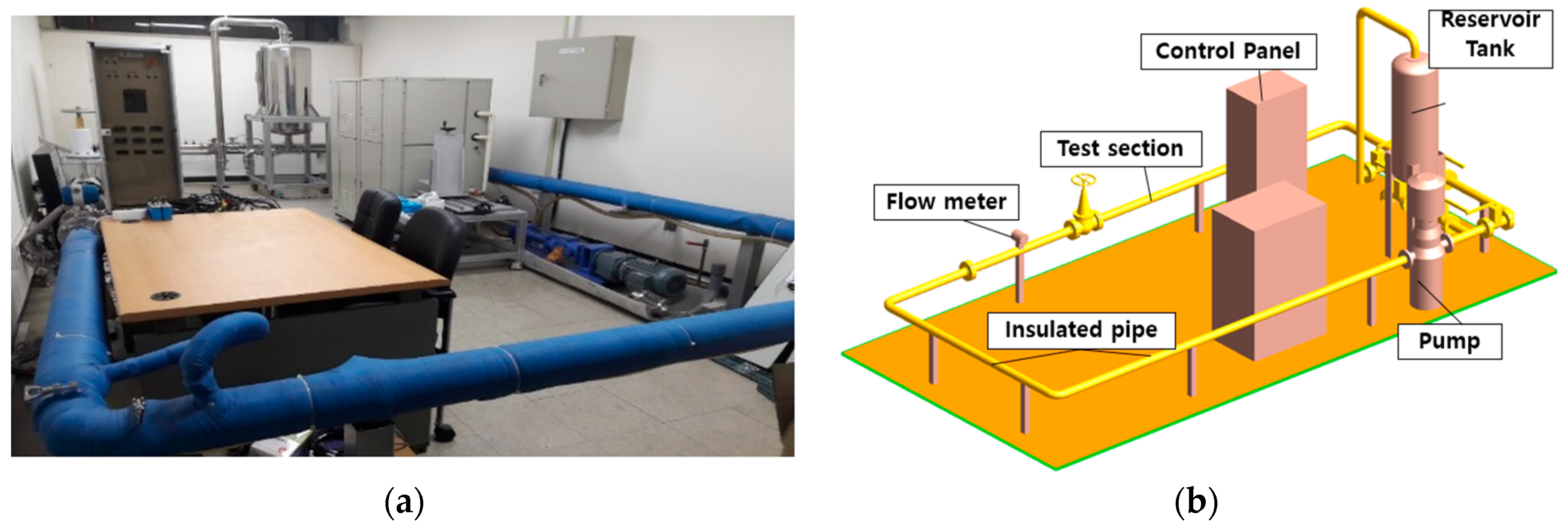
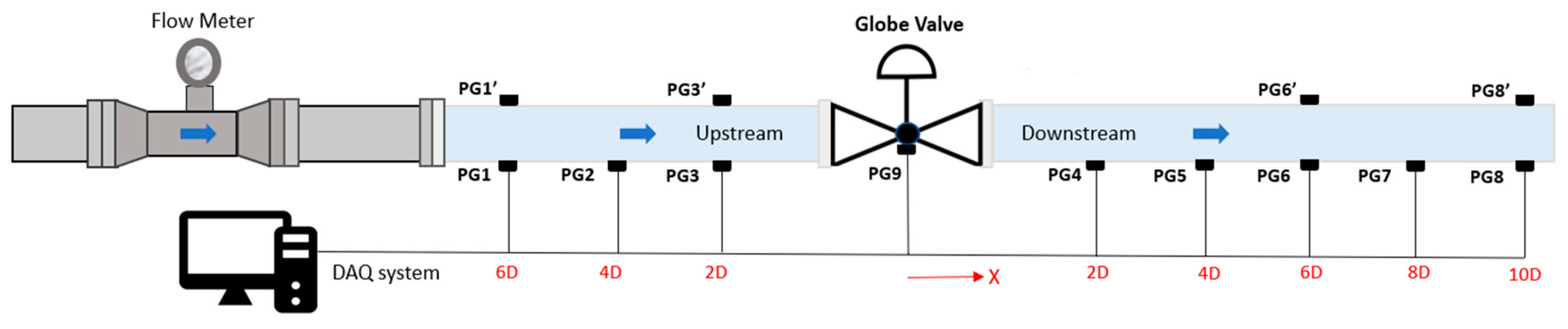
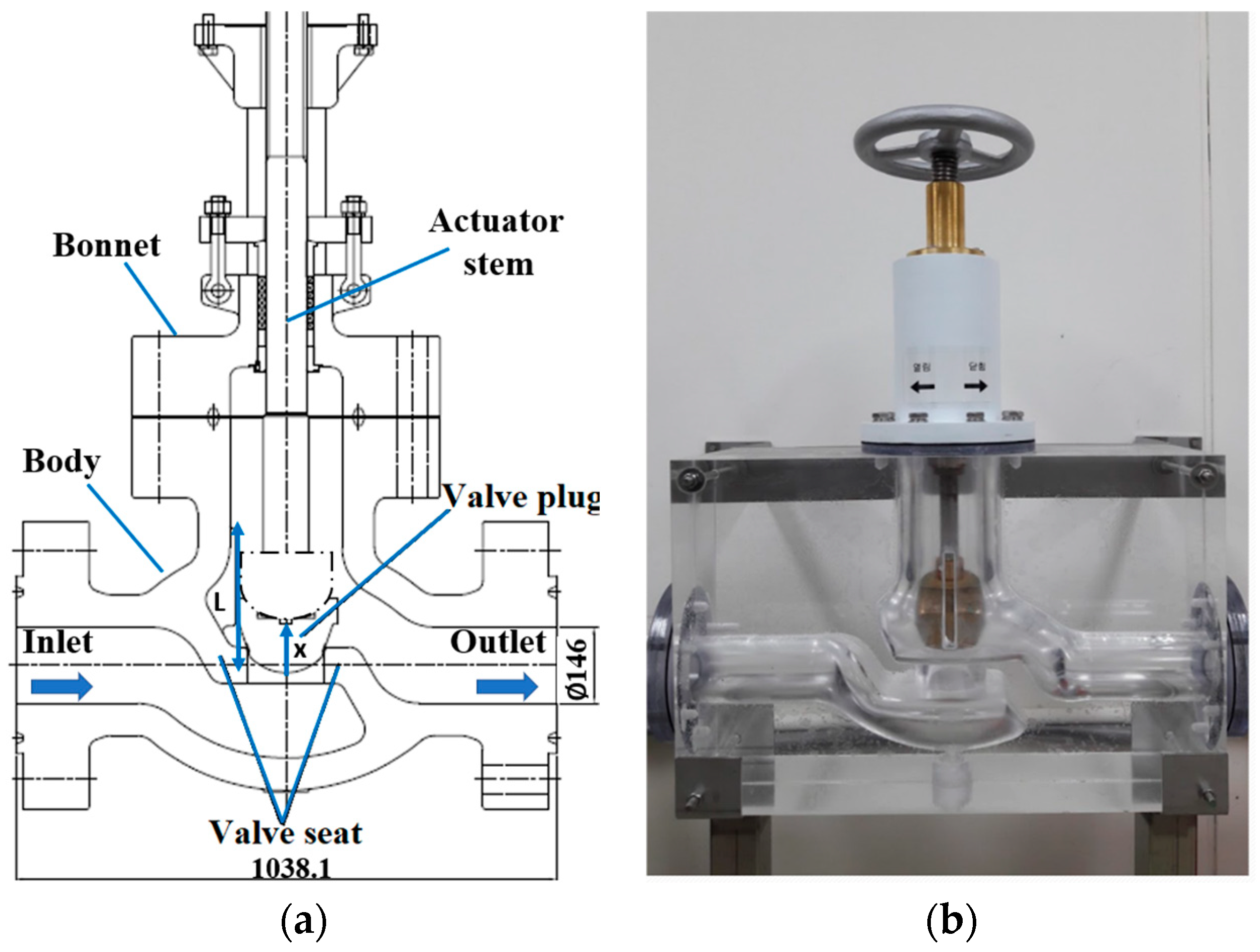
2.1. Experimental Setup

The experiments were conducted in the flow loop which is located at Pusan National University (Figure 1). This loop consists of a reservoir tank, pump, flow meter, and a test section with a three-inch nominal diameter pipeline and total length of 18 m. The flow rate for the flow loop was generated by a multi-stage centrifugal pump with the maximum pump speed of 3500 RPM.

Table 1. Specification of flow loop test facilities.

Reservoir Tank	Net Volume of $20{ \mathrm{m}}^3$
Pump	5.5 kWh, Motor speed: 0–3500 RPM
Total length	18 m, stainless steel pipe
Test section	4 m, acrylic plastic pipe
Pipe diameter	3″

summarizes the specification of the facilities.

The test section is a 4-m acrylic pipe. A series of Kistler 4043A2 piezo-resistive pressure gauge were equally spaced along the bottom of pipeline from the upstream to the downstream of the valve (Figure 2). Four pressure gauges were installed on the top of pipeline to investigate the distribution of pressure difference between the top and the bottom of the same cross-section. Note that the pressure gauge 3 (PG3) at 2D (D: nominal diameter) inlet and PG6 at 6D outlet are the pressure tap positions recommended by the ANSI/ISA-75.01-2012 standard [17].

The sampling frequency was selected at 1000 Hz for pressure measurement and a vortex-type flow meter was installed 10D away from the valve inlet. The specifications of the pressure sensor and the flow meter are listed in

Table 2. Specification of the pressure sensor and flow meter.

	Pressure Sensor	Flow Meter
Sensor	KISTLER 4043A2	KTV-700
Type	Piezo-resistive	Vortex
Range	0–2 bar (abs)	10–100 (${\mathrm{m}}^3/\mathrm{h}$)
Sampling rate	1000 Hz	50 Hz

. The pressure and flow rate were obtained in five minutes and there was one minute of relaxation time before the measurements for the flow to be stable after the valve opening and pump speed change.

The valve model used in the experiment is a straight pattern (Z-shaped body) globe valve which has nominal diameter of 3 inches. The prototype is an eight-inch sized globe valve designed according to ANSI B16.11—Class 2500#, which has scale ratio of 2.7:1 (Figure 3).

2.2. Experimental Conditions

The globe valve was tested at various valve openings, which indicate how far the valve plug was moved relative to its maximum travel [10].

$$\alpha =\frac{x}{L}\times 100\%$$

(1)

where $\alpha$ denotes the valve opening (%), $x$ is the valve travel from the fully closed position, and $L$ is the maximum valve travel (Figure 3a). The valve model used in this study has the plug movement in the range of 0~5 cm, and the valve opening increments is 0.5 cm.

The test investigates the flow coefficient, which builds the flow characteristic of a valve. The flow characteristics of a valve can be referred as inherent characteristics if the pressure drop across the valve is kept constant. Otherwise, they can be referred as installed characteristics if the pressure drop is influenced by the varying process conditions. There are three most common flow characteristics of a valve which are called quick (fast) opening type, linear type and equal percentage type [18].

• Quick opening type produces a large increase in flow rate for initial increase in valve opening and is usually used for safety or cooling systems where the instant large flow is required.
• Linear type has a linear relationship between the flow rate and the valve opening that is commonly used in liquid level control applications.
• Equal percentage type provides a small increase in flow rate with the initial valve openings and a significant rise with the greater openings and is widely found in pressure control and heat transfer processes.

The relationship between valve opening and flow rate through the valve is described quantitively as Equation (2) [17].

$$K_v=Q\sqrt{\frac{SG}{\Delta P}}$$

(2)

where $Q$ and $\Delta P$ are the flow rate $\left({\mathrm{m}}^3/\mathrm{h}\right)$ and the pressure drop (bar) through the valve, and $SG$ is the specific gravity. The pressure drop was measured between pressure gauge PG3 and PG6, which are 2D from the upstream and 6D from the downstream of the valve (Figure 2). It is noted that the $K_v$ in the valve data sheet provided by valve manufacturers is the inherent flow coefficient where the test is performed in constant pressure drop condition [19]. However, when valves are installed in a piping system, the pressure drop across the valve is not a constant as in laboratory condition due to the interactions between the valve and pumps, elbows, and other pressure-consuming components. The installed characteristics include the effects of piping loss and the pump characteristics that cause the different pressure drop in comparison with the inherent flow coefficient of the valve [5]. In this study, both kinds of the flow coefficients were measured and compared with different experimental conditions for each characteristic as shown in

Table 3. Experimental conditions for measurement of flow coefficients.

Valve Opening	Inherent Characteristic	Installed Characteristic
		Pump Speed
10–100% (every 10%)	Constant pressure drop	1000–2000 rpm
	0.069 bar (1 psi); 0.1 bar; 0.13 bar	(every 100 rpm)

.

3. Results and Discussion

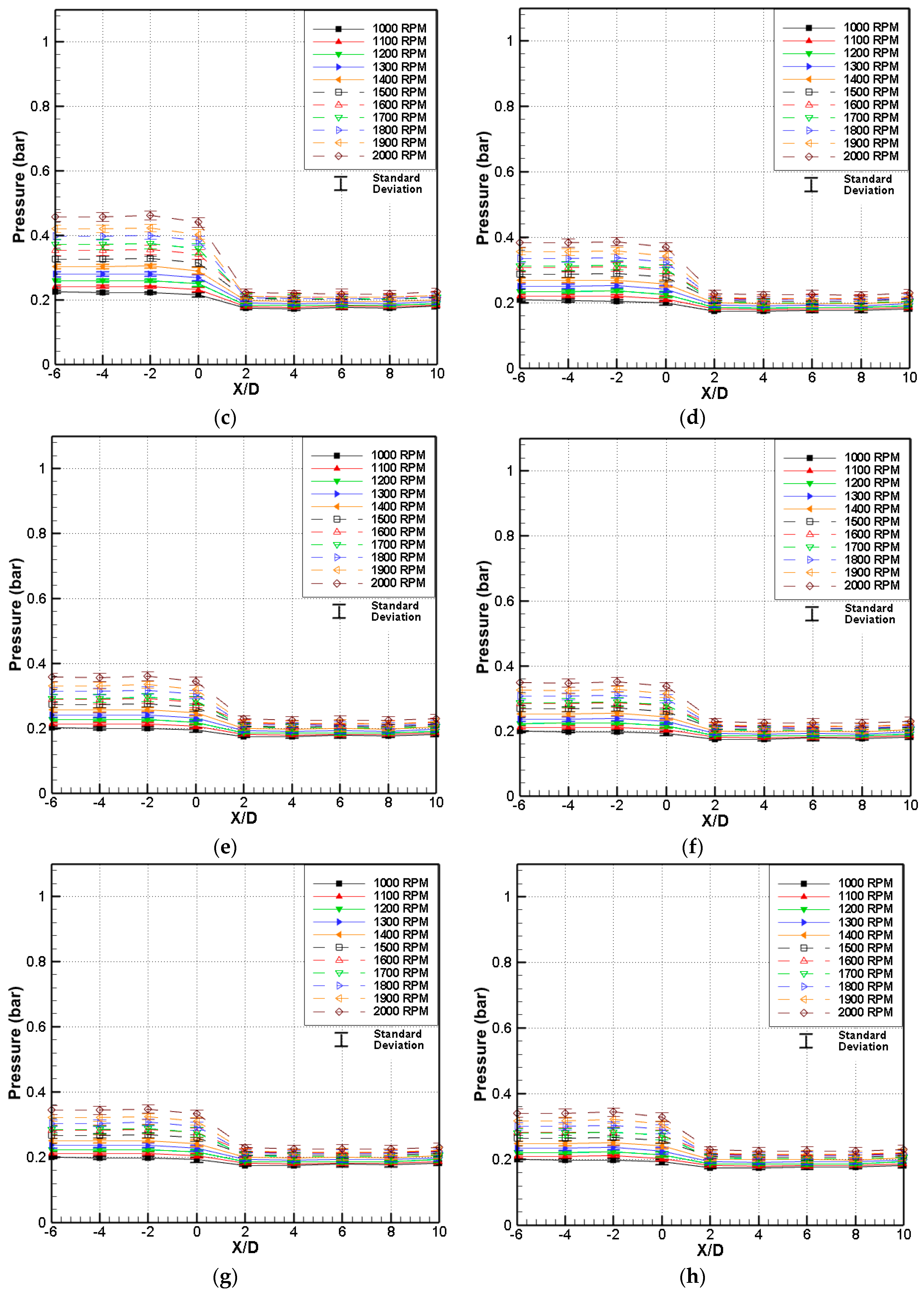
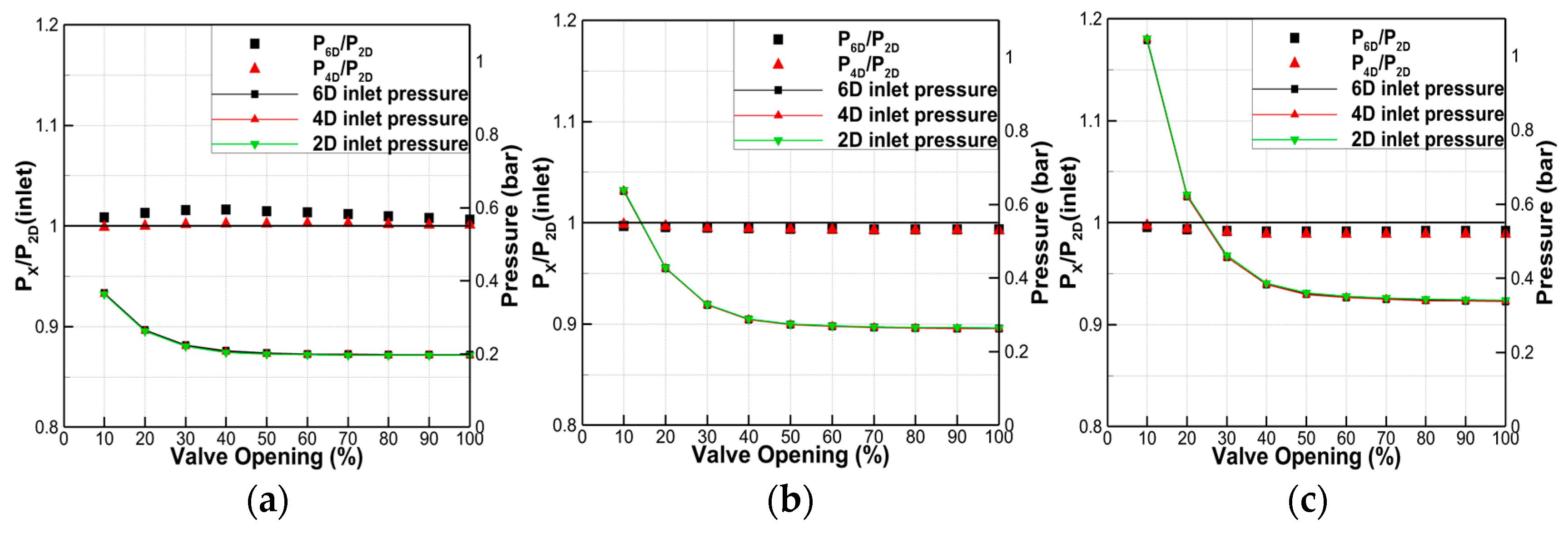
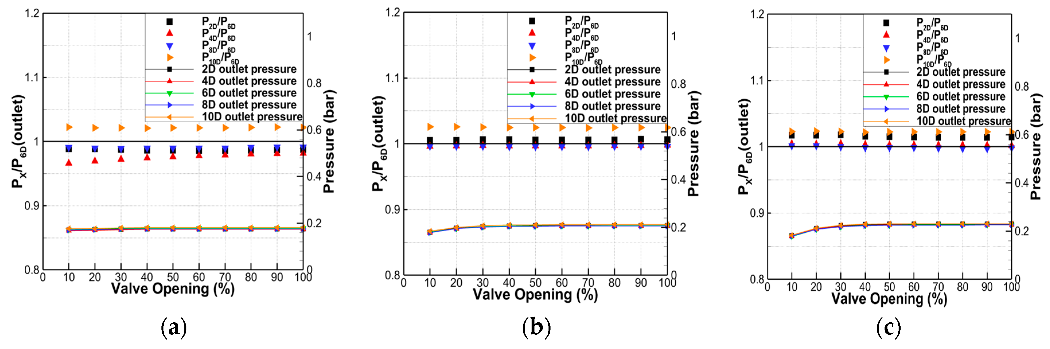
3.1. Pressure Distribution

Figure 4 shows the pressure distributions along the pipeline during the operation with various pump speeds (from 1000 RPM to 2000 RPM) and valve openings (from 10% to 100%). The pressures are presented as the averaged values of five minutes measurement, and the error bars mean the standard deviation of 95% of confidence interval.

In Figure 4, the pressures obtained in the upstream of the valve (from −6 of X/D to −2) show similar magnitudes along the pipe and starts to drop at the bottom of valve (X/D = 0). The pressures rapidly decrease after the plug of the valve and level off along the measurement positions in the downstream of the pipeline (from 2 of X/D to 10). The amount of pressure drop is significant with 10% (Figure 4a) and 20% (Figure 4b) of valve opening due to the relatively small orifice inside the valve. The pressure drop reaches the maximum at the highest pump speed (2000 RPM) with the largest magnitude of the standard deviation due to the complex interaction between the water flow and the globe valve.

Figure 5 shows the pressure drops at the globe valve with various valve opening degrees and pump speeds. The pressure drops in the experiments are the differences between the averaged pressure measured at 2D away from valve inlet (PG3) and 6D away from valve outlet (PG6) based on the recommendation of ANSI/ISA-75.01-2012 standards [17]. It is observed that the pressure drops at the globe valve have a exponentially descending pattern with the linear increase of the valve opening and are proportional with the pump speed. The pressure drops level off from the valve opening of 50%, which represented the quick opening characteristic valve that has been discussed in Section 2.2.

To investigate the effect of pressure measurement positions on the pressure drop term in calculation of flow coefficient (Equation (2)), the pressures at various positions in the upstream and downstream of the valve were measured synchronously, and compared in Figure 6 and Figure 7. Figure 6 correlates the averaged pressures at the upstream and its ratio to the 2D from the valve inlet (PG3), where the ANSI/ISA-75.01 standard [17] recommended, with various pump speeds (1000, 1500, and 2000 RPM). Figure 7 compares the pressures along the downstream, at 6D from the valve outlet (PG6). The ratios of the measured pressures at the recommended locations by ANSI/ISA-75.01 increase slightly with the increasing distance between the measurement position and the reference position. Besides, the ratios vary with the change of the pump speed, which show larger ratios with smaller pump speeds. The largest magnitude of the ratio is at 10D from the valve outlet, when the pump speed is 1000 RPM. Except this measurement, the differences between the measured pressures at various locations and the reference pressures were lower than 4%. Meanwhile, the magnitude of the ratios is almost 1 for all valve openings and pump speeds. This means that there are no considerable effects of the pressure measurement position on the calculation of pressure drop of the valve, if the positions are within 6D from the valve inlet and 10D from the valve outlet.

Figure 8 shows the comparison of the averaged pressures measured at the top and bottom of the same cross-sections along the pipeline. The averaged pressures measured at the upstream of the pipeline are almost similar, but the differences in pressure increase along the downstream of the pipeline and have the maximum difference at the 10D from the valve outlet. The differences might be caused by the circulation of the flow passing the globe valve [3]. The water is obstructed when it flows in the throat path between the valve plug and valve seat, but the flow is not able to change its direction suddenly and, as a consequence, the back flow appeared near the throat path. The vortex affects the similar pressures on the top and bottom of the pipeline in the region adjacent to the valve. As the circulation gets weaker passing through along the pipeline, the discrepancy in pressure at two sides of the pipeline increased.

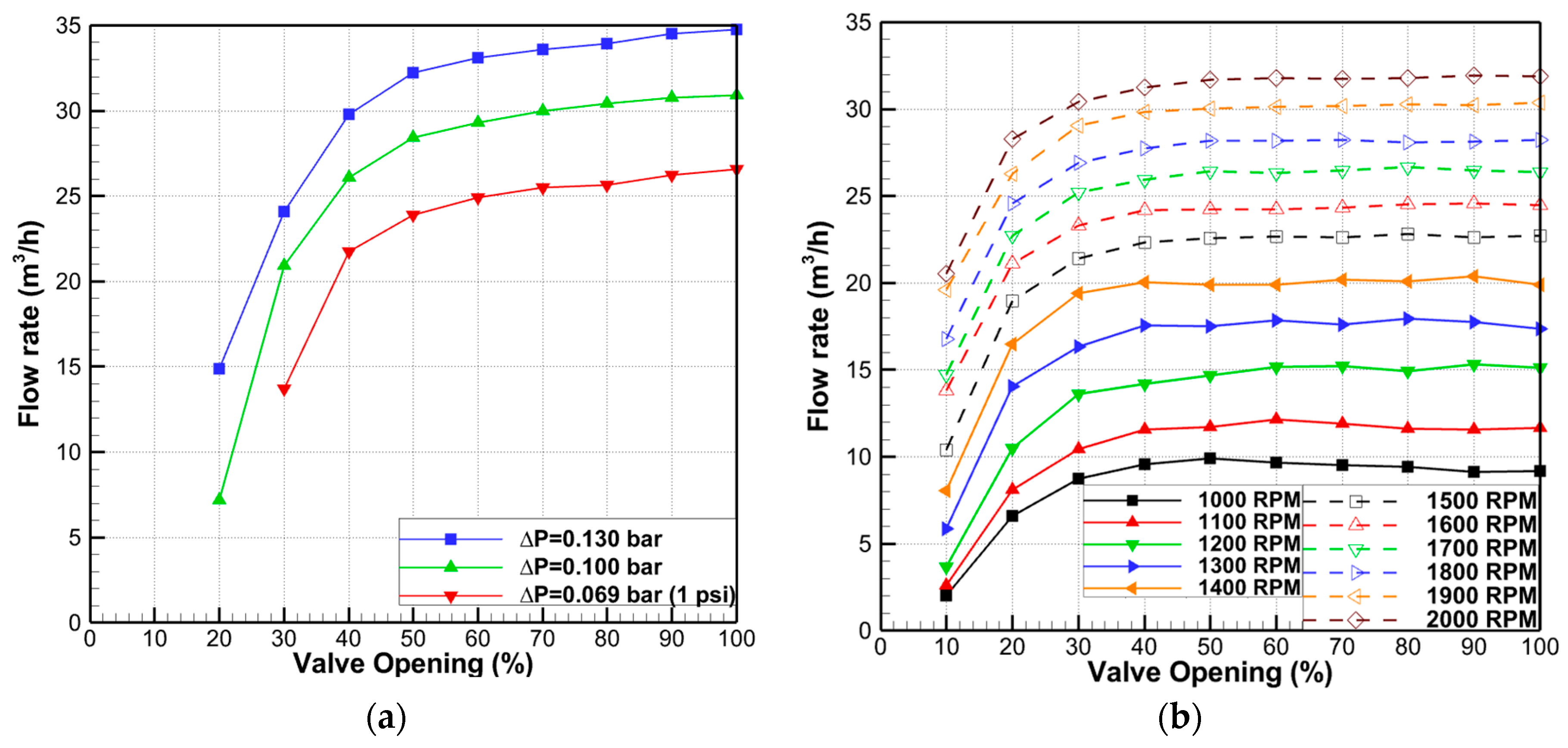
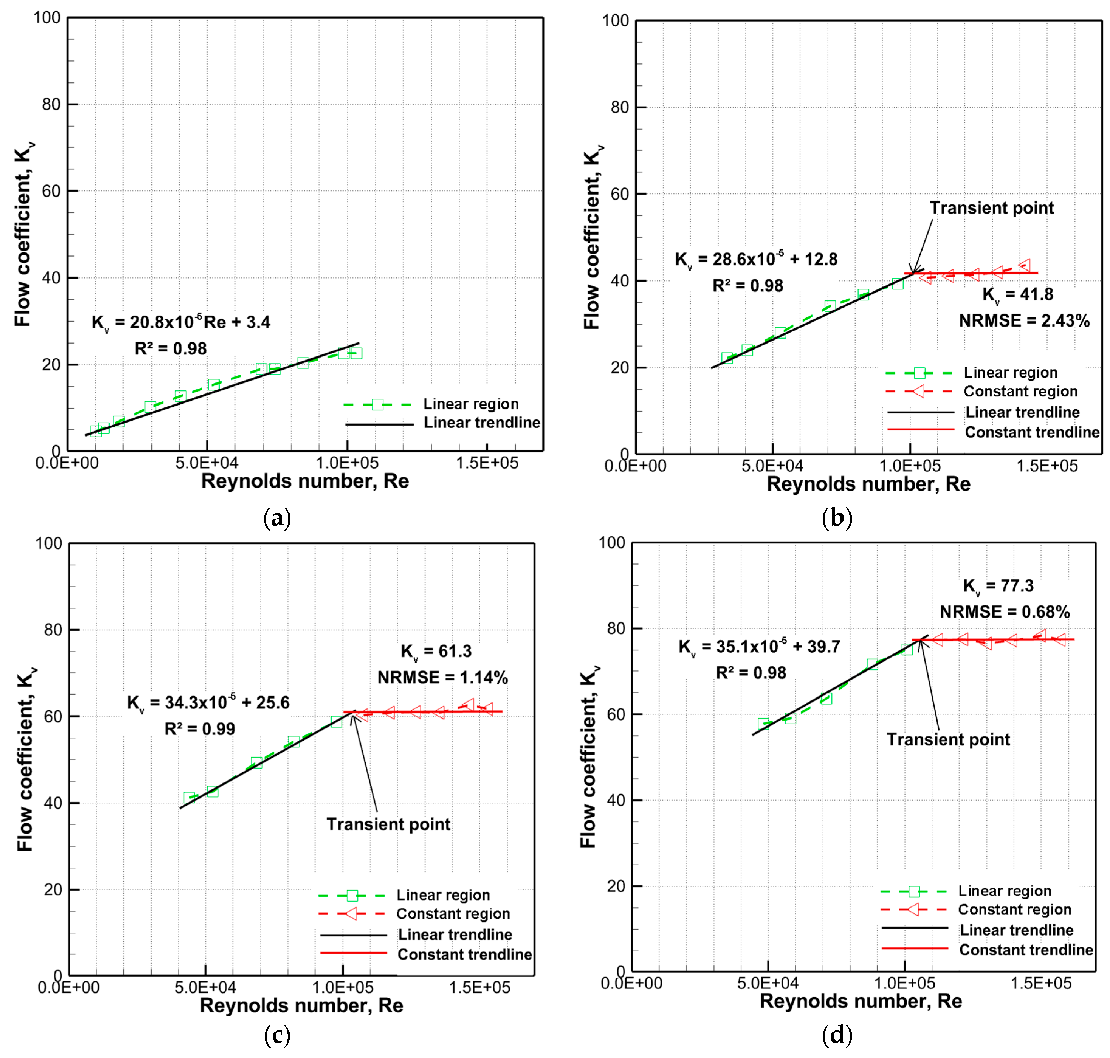
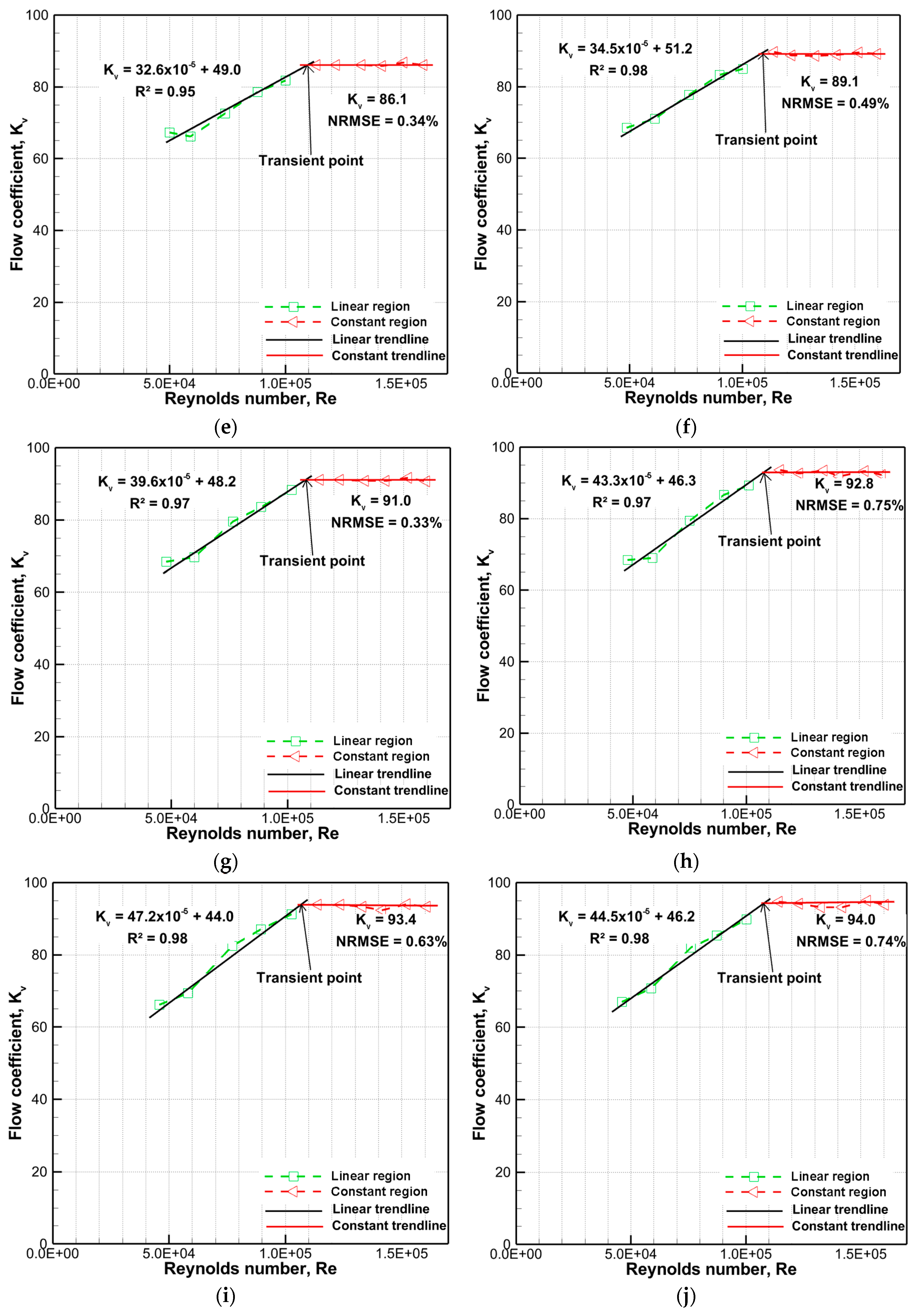
3.2. Flow Characteristics and Flow Coefficient

It is essential to understand various types of flow characteristics and the difference between inherent and installed characteristics in order to choose the proper valve for the system. Figure 9 presents the measured inherent flow characteristics under three different constant pressure drop (Figure 9a) and installed flow characteristics with changing the pump speed (Figure 9b). The inherent flow characteristic showed that the globe valve used in the study has quick opening property which gets more than 80% of maximum flow rate with initial 40% of valve opening. With the pressure drops of 0.069 bar (red line), 0.1 bar (green line), and 0.13 bar (blue line), the flow rates increase but the shape of flow characteristic is flat as in the quick opening condition. This fact hints and confirms that the flow characteristics can be determined from the valve geometry [19].

The quick opening characteristic is also observed in the measurement of the installed condition that reflects the effect of the piping system including the pump and the pipeline layout which causes the pressure loss due to friction. Note that the flow rates in the inherent condition continuously increase with the increasing valve opening (Figure 9a), but the flow rates in the installed condition almost reach the maximum value at 40% valve opening (Figure 9b). The discrepancy between these two flow characteristics is focused in Figure 10. As the valve flow rate is a function of both the valve characteristics and the pressure drop across the valve, conducting inherent flow characteristic test at a constant pressure drop provides a systematic way of comparing one valve characteristic design to another. Meanwhile, the installed characteristic reflects the real response of flow through the valve with a specific system. Figure 10 shows a shift in flow characteristics of an inherent quick opening valve (green line) to an even more quick characteristic of the installed one (red line). There is a significant discrepancy between the inherent characteristic and the installed characteristic of the valve even though they might show the same characteristic as the quick opening characteristic of the valve in this study.

Figure 11 presents the flow coefficients of the globe valve in inherent flow condition (∆P = constant) regarding to the valve opening and the Reynolds number,

$$Re=\frac{VD}{\nu }$$

(3)

where $V$ and $D$ are the average velocity of the flow and the pipe diameter, and $\nu$ is the dynamic viscosity of the fluid. The flow coefficients with changing valve opening in inherent flow condition (Figure 11a) show the convergent tendency with various pressure drops, except the flow coefficients in red circles, which have the corresponding Reynolds number lower than ${10}^5$ as shown in Figure 11b. The flow coefficients seem to level off for Re greater than ${10}^5$.

The convergent tendency of flow coefficients at high Reynolds number is also observed in installed condition with numerous data points at each valve openings as shown in Figure 12. This tendency is similar with the characteristic of the friction factor in Moody diagram [20] and the loss coefficient with respect to Re [21]. Valdes [12] also suggested that the discharge coefficient with respect to Reynolds number has the following trend: a linear increase with Re for purely viscous flow and an asymptotical increase in the transient regime towards the constant value. In this study, the flow coefficient curves at each valve opening (11 data points for each curve) are divided into two regions of linear-trend and constant-trend by the red line shown in Figure 12b. Data fitting based on the linear least squares method is conducted for the linear region, and the coefficient of determination $R^2$ as Equation (4) is used to evaluate the linearity. For the constant region, the horizontal lines crossing the averaged values of the data points are generated, and the differences are evaluated by the Normalized Root Mean Square Error (NRMSE) as Equation (5).

$$R^2=1-\frac{{{\displaystyle \sum }}_i{(y_i-f_i)}^2}{{{\displaystyle \sum }}_i{(y_i-\overline{y})}^2}$$

(4)

$$NRMSE=\frac{1}{\overline{y}}\sqrt{\frac{{\displaystyle \sum }{\left(y_i{-f}_i\right)}^2}{N}}$$

(5)

$$\overline{y}=\frac{1}{N}{\displaystyle \sum }_{i=1}^N{y}_i$$

(6)

where N is the number of data points (N = 11 in this study), $y_i$ is the measured data points and $f_i$ is the regression prediction points. Then, the transients points are determined that are the intersection between the two trendlines.

Table 4. Linearity and constant characteristics of flow coefficient with Reynolds number.

Valve Opening	Linear Trendline		Constant Trendline
	Slope	${\mathit{R}}^2$	${\mathit{K}}_{\mathit{v}\mathit{a}}*$	NRMSE(%)	$\mathit{R}{\mathit{e}}_{\mathit{T}\mathit{P}}*$
10	$20.8\times {10}^{-5}$	0.98
20	$28.6\times {10}^{-5}$	0.99	41.8	2.43	$1.01\times {10}^5$
30	$34.3\times {10}^{-5}$	0.99	61.3	1.14	$1.04\times {10}^5$
40	$35.1\times {10}^{-5}$	0.98	77.3	0.68	$1.07\times {10}^5$
50	$32.6\times {10}^{-5}$	0.95	86.1	0.34	$1.14\times {10}^5$
60	$34.5\times {10}^{-5}$	0.98	89.1	0.49	$1.10\times {10}^5$
70	$39.6\times {10}^{-5}$	0.97	91.0	0.33	$1.08\times {10}^5$
80	$43.3\times {10}^{-5}$	0.97	92.8	0.75	$1.07\times {10}^5$
90	$47.2\times {10}^{-5}$	0.98	93.4	0.63	$1.05\times {10}^5$
100	$44.5\times {10}^{-5}$	0.98	94.0	0.74	$1.08\times {10}^5$

* $K_{va}$ is the average flow coefficients of the constant regions and $R{e}_{TP}$ is the Reynolds number of the transient points.

summaries the data fitting results in which the $R^2$ and $\mathit{NRMSE}$ show the good measurements for linear trendlines and constant trendlines, respectively. Figure 13 shows the linear regions, the transient points and the constant regions of the flow coefficients at each valve opening. All transient points have the Reynolds number between $1.00\times {10}^5$ and $1.15\times {10}^5$. The flow coefficient at 10% valve opening only shows the linear characteristic for the fact that all its data points are in low Reynolds number region, i.e., below ${10}^5$. With the same applied hydraulic pressure range from 0 bar to 2 bar (Table 2), the tests with the other valve opening could successfully obtain the data points in the region of steady flow coefficients. Meanwhile, the tests with the opening of 10% could not obtain any data points due to the high resistance of the valve.

The slopes of linear trendlines of linear regions and the average flow coefficients of the constant regions of flow coefficient with respect to Reynolds number are shown in Figure 14. The slopes have a linear increase trend with the increase in valve opening (Figure 14a). This indicates that in the region of low Reynolds number (below ${10}^5$) for the same increase in Re the larger valve opening the greater increase in flow coefficient. The averaged flow coefficients at each valve opening in the constant regions increase with valve opening (Figure 14b) and its shape confirms the quick opening characteristic as discussed in the first part of this section. From 50% valve opening, the change in flow coefficient is negligible and $K_{vc}$ matches very well with a polynomial function as shown in Figure 14b. Equations (7) and (8) show the curve fitting equations for the slope of the linear trendlines and the average flow coefficients with respect to valve opening.

$$m_{Re}=0.3\times {10}^{-5}\alpha +21.3\times {10}^{-5}.$$

(7)

$$\{\begin{array}{cc}{K}_{va}=1.8\alpha +5.7\hfill & \alpha \le 40\hfill \\ K_{va}=0.0002{\alpha }^3-0.042{\alpha }^2+3.50\alpha -6.7,\hfill & 40<\alpha \hfill \end{array}$$

(8)

where $m_{Re}$ denotes the slope of the linear trendlines of the flow coefficient with a subscript $Re$ for Reynolds number, $\alpha$ is the valve opening and, $K_{va}$ is average flow coefficients of constant regions.

4. Conclusions

In this paper, the pressure distribution and flow characteristics of single-phase water flow through the globe valve are experimentally studied. The pressures at various positions along the pipeline in the upstream and downstream of the test valve are measured and the comparison to pressures at 2D inlet and the 6D outlet, which are the reference taps recommended by ANSI/ISA-75.01 standard, is undertaken. The flow coefficients in both inherent and installed conditions provide some insight into the flow characteristic of the valve in order to select the proper valve for the specific piping applications.

The comparison between measured pressures at different positions to the reference taps shows that there is no significant influence of the pressure measurement locations on the calculation of pressure drop across the valve, if the location is in the vicinity of the valve, within the range 6D from the valve inlet and 10D from outlet. However, the pressure drops across the globe valve are considerable, especially with small valve openings due to the small circulation flow area and the sudden change of the flow direction when the fluid flows in the valve throat. As a result of the circulation, flow occurred inside of the valve and diminished gradually on the valve downstream, the difference in pressure at the top and bottom of the same cross-section along the downstream pipeline might be increased.

The primary performance parameter of a valve is the flow coefficient $K_v$, which is generally a function of valve geometry and the Reynolds number. Sometimes, the dependence on Reynolds number was ignored and a constant flow coefficient was used to calculate the flow rate in valves. However, in order to accurately calculate and size the valve in system, the valve flow coefficient should be investigated as a function of the Reynolds number. In this study, the flow coefficients of a globe valve are investigated for a wide range of Reynolds number. The finding are summarized as follows:

• The flow coefficients increase linearly in low Reynolds number region and level off at the transient points having Re between $1.00\times {10}^5$ and $1.15\times {10}^5$;
• When Re is below ${10}^5$, the flow coefficient grows faster with large valve openings, for the same increase in Reynolds number;
• The flow coefficient increases significantly with the low valve openings with a nearly linear relationship. Meanwhile, additional increases in valve opening give considerable decreases in flow coefficient.

References

1. Rennels, D.C.; Hudson, H.M. Valve. In Pipe Flow: A Practical and Comprehensive Guide, 1st ed.; Wiley: Hoboken, NJ, USA, 2012; pp. 205–212. [Google Scholar]
2. Cho, T.D.; Yang, S.M.; Lee, H.Y.; Ko, S.H. A Study on the Force Balance of an Unbalanced Globe Valve. JMSE 2007, 21, 814–820. [Google Scholar] [CrossRef]
3. Yang, Q.; Zhang, Z.; Hu, J. Numerical Simulation of Fluid Flow inside the Valve. Procedia Eng. 2011, 23, 543–550. [Google Scholar] [CrossRef] [Green Version]
4. Chern, M.J.; Wang, C.C.; Ma, C.H. Numerical Study on Cavitation Occurrence in Globe Valve. J. Energy Eng. 2013, 139, 25–34. [Google Scholar] [CrossRef]
5. Monsen, J. Control Valve Application Technology: Techniques and Considerations for Properly Selecting the Right Control Valve, 1st ed.; Valin Corporation: San Jose, CA, USA, 2013; pp. 17–32. [Google Scholar]
6. Instrument Society of America. Control Valve Sizing Equations for Incompressible Flow; ISA-S39.1 Standard; Research Triangle Park: Durham, NC, USA, 1972. [Google Scholar]
7. Instrument Society of America. Control Valve Sizing Equations; ASNI/ISA-S75.01 Standard; Research Triangle Park: Durham, NC, USA, 1981. [Google Scholar]
8. The American Petroleum Institute (API). Sizing, Selection, and Installation of Pressure-relieving Devices, 9th ed.; API Standard 520; API Publication: Washington, DC, USA, 2013. [Google Scholar]
9. Rahmeyer, W.; Driskell, L. Control Valve Flow Coefficients. J. Transp. Eng. 1985, 111, 358–364. [Google Scholar] [CrossRef]
10. Davis, J.A.; Stewart, M. Predicting Globe Control Valve Performance—Part I: CFD Modeling. J. Fluids Eng. 2002, 124, 772–777. [Google Scholar] [CrossRef]
11. Davis, J.A.; Stewart, M. Predicting Globe Control Valve Performance—Part II: Experimental Verification. J. Fluids Eng. 2002, 124, 778–783. [Google Scholar] [CrossRef]
12. Valdes, J.R.; Rodriguez, J.M.; Saumell, J.; Putz, T. A methodology for the parametric modelling of the flow coefficients and flow rate in hydraulic valves. Energy Conver. Manag. 2014, 88, 598–611. [Google Scholar] [CrossRef]
13. Hollinghead, C.D.; Johnson, M.C.; Barfuss, S.L.; Spall, R.E. Discharge coefficient performance of Venturi, standard concentric orifice plate, V-cone and wedge flow meters at low Reynolds numbers. J. Pet. Sci. Eng. 2011, 78, 559–566. [Google Scholar] [CrossRef]
14. Mu, Y.; Liu, M.; Ma, Z. Research on the measuring characteristics of a new design butterfly valve flowmeter. Flow Meas. Instrum. 2019, 70, 101651. [Google Scholar] [CrossRef]
15. Ferreira, J.P.B.C.C.; Martins, N.M.C.; Covas, D.I.D. Ball Valve Behavior under Steady and Unsteady Conditions. J. Hydraul. Eng. 2018, 144, 04018005. [Google Scholar] [CrossRef]
16. Wu, H.; Li, J.Y.; Gao, Z.X. Flow Characteristics and Stress Analysis of a Parallel Gate Valve. Processes 2019, 7, 803. [Google Scholar] [CrossRef] [Green Version]
17. International Society of Automation. Flow Capacity—Sizing Equations for Fluid Flow under Installed Conditions; ANSI/ISA-75.01.01-2012 Standard; Research Triangle Park: Durham, NC, USA, 2012. [Google Scholar]
18. Control Valve Characteristics. Available online: https://www.spiraxsarco.com/learn-about-steam/control-hardware-electric-pneumatic-actuation/control-valve-characteristics#article-top (accessed on 1 June 2020).
19. Bauman, H.D. Control Valve Primer: A User’s Guide, 4th ed.; ISA Research Triangle Park: Durham, NC, USA, 2009; pp. 53–61. [Google Scholar]
20. Moody, L.F. Friction factors for pipe flow. Trans. Am. Soc. Mech. Eng. 1944, 66, 671–684. [Google Scholar]
21. Cengel, Y.A.; Cimbala, J.M. Internal Flow. In Flow mechanics: Fundamentals and Applications, 3rd ed.; McGraw-Hill: New York, NY, USA, 2014; pp. 374–381. [Google Scholar]
Figure 1. Two-phase (air-water) flow loop in Pusan National University: (a) flow loop facilities; (b) 3D model.
Processes 08 00875 g001
Figure 2. Schematic of the test section.
Processes 08 00875 g002
Figure 3. Prototype and model of the test valve: (a) eight-inch ANSI B16.11—Class 2500# globe valve; (b) three-inch model globe valve.
Processes 08 00875 g003
Figure 4. Pressure distribution along the pipeline. (a) 10% opening. (b) 20% opening. (c) 30% opening. (d) 40% opening. (e) 50% opening. (f) 60% opening. (g) 70% opening. (h) 80% opening. (i) 90% opening. (j) 100% opening.
Processes 08 00875 g004aProcesses 08 00875 g004bProcesses 08 00875 g004c
Figure 5. Pressure drop at the globe valve.
Processes 08 00875 g005
Figure 6. Comparison of pressure in the valve upstream: (a) 1000 RPM; (b) 1500 RPM; (c) 2000 RPM.
Processes 08 00875 g006
Figure 7. Comparison of pressure in the valve downstream: (a) 1000 RPM; (b) 1500 RPM; (c) 2000 RPM.
Processes 08 00875 g007
Figure 8. Comparison of pressure at the top to the bottom of the pipeline: (a) 1000 RPM; (b) 1500 RPM; (c) 2000 RPM.
Processes 08 00875 g008
Figure 9. Flow characteristic of the globe valve. (a) Inherent condition; (b) installed condition.
Processes 08 00875 g009
Figure 10. Comparison of the inherent and installed characteristics.
Processes 08 00875 g010
Figure 11. Flow coefficient in inherent condition: (a) with respect to valve opening; (b) with respect to the Reynolds number.
Processes 08 00875 g011
Figure 12. Flow coefficient in installed condition: (a) with respect to valve opening; (b) with respect to Renolds number.
Processes 08 00875 g012
Figure 13. Linearity and constant characteristics of flow coefficient with Reynolds number. (a) 10% opening. (b) 20% opening. (c) 30% opening. (d) 40% opening. (e) 50% opening. (f) 60% opening. (g) 70% opening. (h) 80% opening. (i) 90% opening. (j) 100% opening.
Processes 08 00875 g013aProcesses 08 00875 g013b
Figure 14. Flow coefficient characteristics with respect to valve opening: (a) slope of the linear trendlines of linear regions; (b) average flow coefficients of constant regions.
Processes 08 00875 g014