Modular Model Predictive Control upon an Existing Controller

Abstract

The availability of predictions of future system inputs has motivated research into preview control to improve set-point tracking and disturbance rejection beyond that achievable via conventional feedback control. The design of preview controllers, typically based upon model predictive control (MPC) for its constraint handling properties, is often performed in a monolithic nature, coupling the feedback and feed-forward problems. This can create problems, such as: (i) an additional feedback loop is introduced by MPC, which alters the closed-loop dynamics of the existing feedback compensator, potentially resulting in a deterioration of the nominal sensitivities and robustness properties of an existing closed-loop and (ii) the default preview action from MPC can be poor, degrading the original feedback control performance. In our previous work, the former problem is addressed by presenting a modular MPC design on top of a given output-feedback controller, which retains the nominal closed-loop robustness and frequency-domain properties of the latter, despite the addition of the preview design. In this paper, we address the second problem; the preview compensator design in the modular MPC formulation. Specifically, we derive the key conditions that ensure, under a given closed-loop tuning, the preview compensator within the modular MPC formulation is systematic and well-designed in a sense that the preview control actions complement the existing feedback control law rather than opposing it. In addition, we also derive some important results, showing that the modular MPC can be implemented in a cascade over any given linear controllers and the proposed conditions hold, regardless of the observer design for the modular MPC. The key benefit of the modular MPC is that the preview control with constraint handling can be implemented without replacing the existing feedback controller. This is illustrated through some numerical examples.

1. Introduction

In many control applications, preview knowledge is available for improving tracking quality and disturbance rejection. Model predictive control (MPC) is a popular method for incorporating both preview knowledge and constraints, because, in principle [1], the information is incorporated in a systematic fashion. However, a standard preview MPC design is often monolithic in nature, where the constraint, preview, and feedback information are coupled in the associated optimisation (e.g., [2,3,4,5]). In contrast, large-scale industrial plants are often live systems with an operating feedback controller. Re-designing the controller within the MPC framework may be costly and impractical. Thus, it is more attractive to practitioners if the advanced control features, such as preview information and constraint handling, can be retrofitted into their existing feedback controller (e.g., [6]).

One of the popular approaches is the reference governor. The reference governor is an add-on scheme that ensures the satisfaction of the state and control constraints by modifying the set-point to a well-designed closed-loop system [7]. For example, the work by Gilbert and Ong [8], Borrelli et al. [9] proposed a reference governor design that satisfies constraints by adjusting the set-point based on the maximal output admissible set. However, such a design is simple and efficient, but only employing the set-point as the degree-of-freedom could result in a loss of optimality, where the degrees-of-freedom are limited to the reference signal only [10]. Much research in recent years has focused on the development of the reference governor within the predictive control framework. For example, the work by Aghaei et al. [11] showed an MPC-based reference governor design, where a couple of exogenous signals, computed by solving an on-line optimisation, were added onto the reference and control variables of the original closed-loop system for ensuring constraint satisfaction. Work by Klauco [12] developed another MPC-based reference governor design for which a set of future references is optimised based on the prediction of the closed-loop system behaviour.

Nonetheless, a large number of these MPC-based reference governor studies employed the set-point as the only optimisation variable, which could thus lead to a loss in performance and optimality. In addition, in some studies, the reference signal is assumed to be constant or the existing control design was based on a state-feedback controller. For some applications, an output-feedback controller is often employed, which is synthesised using frequency domain techniques for satisfying some robustness and performance specifications given in the frequency domain. As a consequence, this begs the question: is there a systematic way to incorporate the merits of MPC, such as the capability for handling constraint and preview knowledge, into an existing feedback controller? A simplistic proposal might involve a standard MPC formulated around the underlying closed-loop dynamics. However: (i) the MPC computes the decision variables depending on the predictions and current state of the closed-loop dynamics. Therefore, the constraint handling features of the MPC depend upon the predictions of the closed-loop dynamics. Thus, optimising such predictions will introduce an additional feedback loop to the original closed-loop, in turn impacting on the carefully designed properties of the existing controller [13,14]; (ii) coupling the feedback and feed-forward design in the standard MPC results in an ’optimal’ feed-forward compensator with respect to the instantaneous cost function rather than the overall closed-loop behaviour. Consequently, the performance of such a compensator is often poor, as reported in many studies [4,15,16]. In the context of designing a modular MPC upon a given feedback controller, if the preview compensator is not carefully designed in a sense that it only handles the transient of the existing closed-loop, the preview action is then mistakenly corrected by the pre-determined feedback control law, resulting in a deterioration in the performance.

We addressed the former problem in our earlier work [14] by presenting a preview modular MPC layer that is based on a known feedback controller. In short, the pre-determined feedback control law focuses on the frequency domain closed-loop properties, such as sensitivity, whilst the feed-forward input from the modular MPC is purely based on advance knowledge. Without corrections that are linked to the measurements from the plant, the MPC module thus does not, unnecessarily, interact with the feedback loop. In this work, we propose the preview compensator design procedure for the modular MPC formulation. Specifically, we derive the key conditions that ensure the preview gain is systematic and optimal in a sense that the preview compensator from the modular MPC formulation only handles the transient of the closed-loop and, once the steady-state is reached, the preview perturbation input remains at zero. Moreover, we derive results demonstrating that the modular MPC can be implemented upon any given linear feedback controller and the use of an observer on the modular MPC has no effect upon the proposed conditions.

This paper first presents the basic definitions of the model and known output-feedback controller and also the formulation of the modular MPC in Section 2. In Section 3.1, the conditions that guarantee the additional MPC design does not influence the nominal stability and robustness of the closed-loop dynamics are revisited. The novelty of this paper starts in Section 3.2, where we derive a set of conditions that proves the preview compensator within the modular MPC formulation is well-designed and systematic in a sense that the preview compensator only handles the transient of the closed-loop based on the future reference signals. In the rest of Section 3, we also derive results that show that the modular MPC is feasible to implement upon any existing linear controller and the proposed conditions hold, regardless of the observer design for the modular MPC. In Section 4, numerical examples are presented and followed by conclusions in Section 5.

Notation

Let $\mathbb{R}$ and $\mathbb{C}$ denote the real and complex fields, respectively, and let $s\in \mathbb{C}$ denote a complex variable. The space $\mathcal{R}$ denotes the space of proper real-rational transfer function matrices and $k\in \mathbb{Z}$ denotes a sample variable of a discrete-time signal. Let $v^T\in {\mathbb{R}}^{1\times n_v}$ denote the transpose of a vector $v\in {\mathbb{R}}^{n_v}$ and $V^T\in {\mathbb{R}}^{n_y\times n_z}$ is the transpose of a matrix $V\in {\mathbb{R}}^{n_z\times n_y}$. The notation ${\stackrel{{\displaystyle v}}{\to }}_k\in {\mathbb{R}}^{n_v{n}_p}$ denotes the future prediction sequence ${[v_{0|k}^T,v_{1|k}^T...,v_{n_p-1|k}^T]}^T\in {\mathbb{R}}^{n_v{n}_p}$, where $v_{1|k}^T$ denotes the one-step ahead predictions at step k. Let $\lambda \left(V\right)\in \mathbb{C}$ denote the eigenvalues of the matrix V.

2. Preliminaries: Modular MPC Design upon an Existing Controller

This section revisits some preliminaries on the modelling assumption and the modular MPC design.

2.1. System and the Existing Controller Models

Assume that the linear model of the plant $G\left(s\right)\in {\mathcal{R}}^{n_y\times n_u}$ is a strictly proper function, which can be described in discrete-time state-space forms, as follows:

$$\begin{array}{c}\hfill x_{{\mathrm{p}}_{k+1}}=A_{\mathrm{p}}{x}_{{\mathrm{p}}_k}+B_{\mathrm{p}}{u}_k;y_k=C_{\mathrm{p}}{x}_{{\mathrm{p}}_k},\end{array}$$

(1)

where $u_k\in {\mathbb{R}}^{n_u}$, $y_k\in {\mathbb{R}}^{n_y}$ and $x_{{\mathrm{p}}_k}\in {\mathbb{R}}^{n_{x_{\mathrm{p}}}}$ represent the input, output, and state of the plant, respectively, whilst the subscript $\mathrm{p}$ denotes the plant.

Let the existing output-feedback controller stabilising the linear model (1) and track the set-point $r_k\in {\mathbb{R}}^{n_y}$ be given by $K\left(s\right)\in {\mathcal{R}}^{n_u\times n_y}$, with its discrete-time state-space form. as follows:

$$\begin{array}{cc}\hfill x_{{\kappa }_{k+1}}& =A_{\kappa }{x}_{{\kappa }_k}+B_{\kappa }(r_k-y_k),\hfill \\ \hfill u_k& =C_{\kappa }{x}_{{\kappa }_k}+D_{\kappa }(r_k-y_k),\hfill \end{array}$$

(2)

where the vector $x_{{\kappa }_k}\in {\mathbb{R}}^{n_{x_{\kappa }}}$ represents the state of the controller and the subscript $\kappa$ denotes controller.

To achieve offset-free control from the modular MPC, it is convenient to express the system (1) and controller (2) model in terms of the deviation variables, defined as follows:

$$\begin{array}{cc}\hfill {\tilde{x}}_{{\mathrm{p}}_{k+1}}& =A_{\mathrm{p}}{\tilde{x}}_{{\mathrm{p}}_k}+B_{\mathrm{p}}{\tilde{u}}_k;{\tilde{y}}_k=C_{\mathrm{p}}{\tilde{x}}_{{\mathrm{p}}_k},\hfill \end{array}$$

(3a)

$$\begin{array}{cc}\hfill {\tilde{x}}_{{\kappa }_{k+1}}& =A_{\kappa }{\tilde{x}}_{{\kappa }_k}-B_{\kappa }{\tilde{y}}_k;{\tilde{u}}_k=C_{\kappa }{\tilde{x}}_{{\kappa }_k}-D_{\kappa }{\tilde{y}}_k,\hfill \end{array}$$

(3b)

where the deviation of the plant state ${\tilde{x}}_{\mathrm{p},k}=x_{\mathrm{p},k}-x_{\mathrm{p},k}^{\mathrm{s}}$, the controller state ${\tilde{x}}_{\kappa ,k}=x_{\kappa ,k}-x_{\kappa ,k}^{\mathrm{s}}$, the input ${\tilde{u}}_k=u_k-u_k^{\mathrm{s}}$ and the output $\tilde{y}=y_k-r_k$ are with respect to their steady-state $x_{\mathrm{p},k}^{\mathrm{s}},x_{\kappa ,k}^{\mathrm{s}},u_k^{\mathrm{s}}$. The steady-states $x_{\mathrm{p},k}^{\mathrm{s}},x_{\kappa ,k}^{\mathrm{s}},u_k^{\mathrm{s}}$, that enable $y\to r_k$ asymptotically, can be calculated from a typical steady-state target calculator (e.g., [17]), defined as follows:

$$\begin{array}{c}\hfill \left[\begin{array}{c}{x}_{\mathrm{p},k}^{\mathrm{s}}\\ x_{\kappa ,k}^{\mathrm{s}}\\ u_k^{\mathrm{s}}\end{array}\right]={\left[\begin{array}{ccc}I-A_{\mathrm{p}}& 0& -B\\ 0& I-A_{\kappa }& 0\\ C& 0& 0\end{array}\right]}^{-1}\left[\begin{array}{c}0\\ 0\\ r_k\end{array}\right]=\left[\begin{array}{c}{K}_{xr}\\ K_{ur}\end{array}\right]r_k.\end{array}$$

(4)

Combining the linear model (3a) and controller (3b), the closed-loop dynamic system model can be expressed in the following form:

$$\begin{array}{cc}\hfill \left[\begin{array}{c}{\tilde{x}}_{\mathrm{p},k+1}\\ {\tilde{x}}_{\kappa ,k+1}\end{array}\right]& =\underset{A}{\underbrace{\left[\begin{array}{cc}{A}_{\mathrm{p}}& 0\\ -B_{\kappa }{C}_{\mathrm{p}}& A_{\kappa }\end{array}\right]}}\underset{{\tilde{x}}_k}{\underbrace{\left[\begin{array}{c}{\tilde{x}}_{\mathrm{p},k}\\ {\tilde{x}}_{\kappa ,k}\end{array}\right]}}+\underset{B}{\underbrace{\left[\begin{array}{c}{B}_{\mathrm{p}}\\ 0\end{array}\right]}}{\tilde{u}}_k,\hfill \end{array}$$

(5a)

$$\begin{array}{cc}\hfill {\tilde{u}}_k& =\left[\begin{array}{cc}-D_{\kappa }{C}_{\mathrm{p}}& C_{\kappa }\end{array}\right]{\tilde{x}}_k=K{\tilde{x}}_k,\hfill \end{array}$$

(5b)

$$\begin{array}{cc}\hfill {\tilde{y}}_k& =\left[\begin{array}{cc}{C}_{\mathrm{p}}& 0\end{array}\right]{\tilde{x}}_k=C{\tilde{x}}_k.\hfill \end{array}$$

(5c)

The pairs $\{A,B\}$ and $\{A,{[C,K]}^T\}$ are assumed be to controllable and observable, respectively.

2.2. Design of the Modular MPC

The working principle of a typical modular MPC is to compute a future perturbation input sequence by solving an optimisation problem that takes into account the closed-loop model prediction, performance index, and constraint. Figure 1 shows the architecture combining the proposed modular MPC and the separate feedback controller, where $u,y$ and r denote the input, output, and reference signal of the plant, respectively. The proposed modular MPC optimises the perturbation c to handle constraints as well as act upon the preview reference signal $\stackrel{{\displaystyle r}}{\to }$.

2.2.1. Augmentation of Perturbation into the Underlying Control Law

The modular MPC formulation in this work adopts a dual-mode closed-loop paradigm (e.g., [18,19]), whereby the degrees-of-freedom (d.o.f) $c_k\in {\mathbb{R}}^{n_u}$ within the predictions are defined around a stabilising feedback control law (5b), such that the input can be parametrised, as follows:

$$\begin{array}{c}\hfill {\tilde{u}}_{i|k}=\left\{\begin{array}{cc}K{\tilde{x}}_{i|k}+c_{i|k},\hfill & \forall i=\{0,\cdots ,n_c-1\},\hfill \\ K{\tilde{x}}_{i|k},\hfill & \forall i\ge n_c.\hfill \end{array}\right.\end{array}$$

(6)

The premise behind this approach is that the MPC perturbation $c_k$ is non-zero if and only if constraints are active or preview knowledge is available; obviously, when $c_k=0$ the underlying feedback controller operates unaffected. Such a feature is particularly useful in formulating a modular MPC on top of a given feedback controller. Notice that the predicted perturbation sequence ${\stackrel{{\displaystyle c}}{\to }}_k={[c_{0|k},c_{1|k},...,c_{n_c-1|k}]}^T\in {\mathbb{R}}^{n_u{n}_c}$ is optimised over the control horizon $n_c$, whilst, beyond $n_c$, the closed-loop dynamics are solely governed by the given feedback control law.

2.2.2. Cost Function and Optimisation Problem

A common cost function is to penalise the weighted squares of the predicted tracking errors and the deviations in control input from its steady-state (e.g., [19]):

$$\begin{array}{c}\hfill J_k=\sum _{i=0}^{\infty }{\tilde{x}}_{i|k}^{T}Q{\tilde{x}}_{i|k}+{\tilde{u}}_{i|k}^{T}R{\tilde{u}}_{i|k},\end{array}$$

(7)

where $Q=Q^T\ge 0\in {\mathbb{R}}^{n_x\times n_x}$ and $R=R^T>0\in {\mathbb{R}}^{n_u\times n_u}$ denote the weighting matrices on state and input, respectively.

Subsequently, the associated optimisation problem that minimises the perturbation sequence ${\stackrel{{\displaystyle c}}{\to }}_k$ is described, as follows:

$$\begin{array}{cc}\hfill \underset{\begin{array}{c}{\stackrel{{\displaystyle c}}{\to }}_k\end{array}}{min}& J_k=\sum _{i=0}^{\infty }{\tilde{x}}_{i|k}^{T}Q{\tilde{x}}_{i|k}+{\tilde{u}}_{i|k}^{T}R{\tilde{u}}_{i|k},\hfill \end{array}$$

(8a)

$$\begin{array}{cc}\hfill \mathrm{s}.\mathrm{t}.& {\tilde{x}}_{i+1|k}=A{\tilde{x}}_{i|k}+B{\tilde{u}}_{i|k},\forall i\ge 0,\hfill \end{array}$$

(8b)

$$\begin{array}{cc}\hfill & {\tilde{u}}_{i|k}=\left\{\begin{array}{cc}K{\tilde{x}}_{i|k}+c_{i|k},\hfill & \forall i=\{0,\cdots ,n_c-1\},\hfill \\ K{\tilde{x}}_{i|k},\hfill & \forall i\ge n_c,\hfill \end{array}\right.\hfill \end{array}$$

(8c)

$$\begin{array}{cc}\hfill & r_{i|k}=\left\{\begin{array}{cc}{r}_{k+i}\hfill & \forall i=\{0,\cdots ,n_a-1\},\hfill \\ r_{k+n_a-1}\hfill & \forall i\ge n_a\hfill \end{array}\right.\hfill \end{array}$$

(8d)

$$\begin{array}{cc}\hfill & u_{i|k}^s=K_{ur}{r}_{i|k},x_{i|k}^s=K_{xr}{r}_{i|k}.\hfill \end{array}$$

(8e)

The predictions of state, input, set-point, and steady-state are denoted by (8b), (8c), (8d), and (8e), respectively. The set-point $r_k$ is assumed to be known for $n_a$ steps into the future and beyond the preview horizon $n_a$, the reference prediction is assumed to hold the last available value $r_{k+i}=r_{k+n_a-1}\forall i\ge n_a$.

2.2.3. Autonomous Prediction Model to Simplify the Optimisation Problem

The predictions of state (8b), input (8c), set-point (8d), and steady-state (8e) can be expressed in a more convenient and compact autonomous prediction model form (e.g., [20]), for which the state $z_{i|k}\in {\mathbb{R}}^{n_z}$ consists of the state $x_{i|k}$ of the model, perturbations ${\stackrel{{\displaystyle c}}{\to }}_k$ and future reference signal ${\stackrel{{\displaystyle r}}{\to }}_k={[r_k,r_{k+1},...,r_{k+n_a-1}]}^T\in {\mathbb{R}}^{n_y{n}_a}$. Thus, the model is defined, as follows:

$$z_{i+1|k}=\mathsf{\Psi }{z}_{i|k},$$

(9a)

where the initial state $z_{0|k}={[x_{0|k},{\stackrel{{\displaystyle c}}{\to }}_k,{\stackrel{{\displaystyle r}}{\to }}_k]}^T$ and $\mathsf{\Psi }$ are defined as:

$$\begin{array}{cc}\hfill \mathsf{\Psi }& =\left[\begin{array}{ccc}\mathsf{\Phi }& BE& (I-\mathsf{\Phi })K_{xr}E\\ 0& M_c& 0\\ 0& 0& M_r\end{array}\right],\hfill \end{array}$$

(9b)

$$\begin{array}{cc}\hfill E{\stackrel{{\displaystyle c}}{\to }}_k& =c_{0|k},E{\stackrel{{\displaystyle r}}{\to }}_k=r_{0|k},\hfill \end{array}$$

(9c)

$$\begin{array}{cc}\hfill M_c{\stackrel{{\displaystyle c}}{\to }}_k^T& ={[c_{1|k},\cdots ,c_{n_c-1|k},0]}^T,\hfill \end{array}$$

(9d)

$$\begin{array}{cc}\hfill M_r{\stackrel{{\displaystyle r}}{\to }}_k^T& ={[r_k,\cdots ,r_{k+n_a-1},r_{k+n_a-1}]}^T,\hfill \end{array}$$

(9e)

where $\mathsf{\Phi }=A+BK\in {\mathbb{R}}^{n_x\times n_x}$ and $\left|\lambda \right(\mathsf{\Phi }\left)\right|<1$, and the shift matrices $M_c\in {\mathbb{R}}^{n_u{n}_c\times n_u{n}_c}$ and $M_r\in {\mathbb{R}}^{n_y{n}_a\times n_d{n}_a}$ are defined as follows:

$$\begin{array}{c}\hfill M_c=\left[\begin{array}{ccccc}0& I& 0& \cdots & 0\\ 0& 0& I& \cdots & 0\\ ⋮& ⋮& ⋮& \ddots & ⋮\\ 0& 0& 0& \cdots & I\\ 0& 0& 0& \cdots & 0\end{array}\right];M_r=\left[\begin{array}{ccccc}0& I& 0& \cdots & 0\\ 0& 0& I& \cdots & 0\\ ⋮& ⋮& ⋮& \ddots & ⋮\\ 0& 0& 0& \cdots & I\\ 0& 0& 0& \cdots & I\end{array}\right],\end{array}$$

(10a)

and $E\in {\mathbb{R}}^{n_x\times n_u{n}_c}$ is described as follows:

$$\begin{array}{c}\hfill E=\left[\begin{array}{ccccc}I& 0& 0& \cdots & 0\end{array}\right].\end{array}$$

(10b)

Lemma 1

(e.g., [20]). The MPC optimisation problem (with equivalent cost function to (8)) and using the autonomous form (9), is given by:

$$\begin{array}{cc}\hfill \underset{{\stackrel{{\displaystyle c}}{\to }}_k}{min}& J_k=\sum _{i=0}^{\infty }{z}_{i|k}^T({\mathsf{\Gamma }}_x^{T}Q{\mathsf{\Gamma }}_x+{\mathsf{\Gamma }}_u^{T}R{\mathsf{\Gamma }}_u)z_{i|k},\hfill \end{array}$$

(11a)

$$\begin{array}{cc}\hfill \mathrm{s}.\mathrm{t}.& z_{i+1|k}=\mathsf{\Psi }{z}_{i|k},\forall i\ge 0,\hfill \end{array}$$

(11b)

where ${\mathsf{\Gamma }}_x=\left[\begin{array}{ccc}I& 0& -K_{xr}\end{array}\right]\in {\mathbb{R}}^{n_x\times n_z}$ and ${\mathsf{\Gamma }}_u=\left[\begin{array}{ccc}K& E& -K{K}_{xr}\end{array}\right]\in {\mathbb{R}}^{n_u\times n_z}$.

Proof. 

The result follows from substitution of (9) into (8). See [20]. □

Corollary 1.

The infinite-horizon cost function in (8) (and thus also (11a)) can be compacted into a finite-horizon form, while using the Lyapunov equation ${\mathsf{\Psi }}^{T}S\mathsf{\Psi }=S-W$ and $z_{i|k}={\mathsf{\Psi }}^i{z}_{0|k}$:

$$\begin{array}{cc}\hfill J_k& =z_{0|k}^T\underset{S}{\underbrace{\sum _{i=0}^{\infty }{{\mathsf{\Psi }}^i}^T\underset{W}{\underbrace{\left({\mathsf{\Gamma }}_x^{T}Q{\mathsf{\Gamma }}_x+{\mathsf{\Gamma }}_u^{T}R{\mathsf{\Gamma }}_u\right)}}{\mathsf{\Psi }}^i}}{z}_{0|k},\hfill \end{array}$$

(12a)

$$\begin{array}{cc}\hfill & ={\left[\begin{array}{c}{x}_{0|k}\\ {\stackrel{{\displaystyle c}}{\to }}_k\\ {\stackrel{{\displaystyle r}}{\to }}_k\end{array}\right]}^{T}S\left[\begin{array}{c}{x}_{0|k}\\ {\stackrel{{\displaystyle c}}{\to }}_k\\ {\stackrel{{\displaystyle r}}{\to }}_k\end{array}\right]={\left[\begin{array}{c}{x}_{0|k}\\ {\stackrel{{\displaystyle c}}{\to }}_k\\ {\stackrel{{\displaystyle r}}{\to }}_k\end{array}\right]}^T\left[\begin{array}{ccc}{S}_x& S_{xc}& S_{xr}\\ S_{xc}^T& S_c& S_{cr}\\ S_{xr}^T& S_{cr}^T& S_r\end{array}\right]\left[\begin{array}{c}{x}_{0|k}\\ {\stackrel{{\displaystyle c}}{\to }}_k\\ {\stackrel{{\displaystyle r}}{\to }}_k\end{array}\right],\hfill \end{array}$$

(12b)

$$\begin{array}{cc}\hfill & ={\stackrel{{\displaystyle c}}{\to }}_k^T{S}_c{\stackrel{{\displaystyle c}}{\to }}_k+2{\stackrel{{\displaystyle c}}{\to }}_k^T{S}_{xc}^T{x}_{0|k}+2{\stackrel{{\displaystyle c}}{\to }}_k^T{S}_{cr}{\stackrel{{\displaystyle r}}{\to }}_k+ϵ,\hfill \end{array}$$

(12c)

where ϵ denotes the terms that are independent of $\stackrel{{\displaystyle c}}{\to }$ and $x_{0|k}=x_k$.

The key point of Corollary 1 is to simplify the infinite-horizon cost function (11a) into the finite-horizon cost (12).

2.2.4. Constraint Formulations in Terms of Perturbations

Let the system be subject to constraints of the form:

$$\begin{array}{ccc}\hfill & y_{\min }\le y_{i|k}\le y_{\max },\hfill & \hfill \forall i\ge 0,\end{array}$$

(13a)

$$\begin{array}{ccc}\hfill & u_{\min }\le u_{i|k}\le u_{\max },\hfill & \hfill \forall i\ge 0.\end{array}$$

(13b)

Given that the state and input is captured in terms of the autonomous form (9), thus, the inequalities (13) can be written, as follows:

$$\begin{array}{ccc}\hfill & H{z}_{i|k}\le h,\hfill & \hfill \forall i\ge 0,\end{array}$$

(14a)

where

$$\begin{array}{cc}\hfill & H{z}_{i|k}={\left[\begin{array}{cccc}{y}_{i|k}& -y_{i|k}& u_{i|k}& -u_{i|k}\end{array}\right]}^T,\hfill \end{array}$$

(14b)

$$\begin{array}{cc}\hfill & h={\left[\begin{array}{cccc}{y}_{\max }& -y_{\min }& u_{\max }& -u_{\min }\end{array}\right]}^T.\hfill \end{array}$$

(14c)

It is noted that to ensure no constraint violations, possible violations in (14) must be checked over an infinite prediction horizon, which would appear to be computationally impractical. However, it is well known [21] that there exists a sufficiently large horizon $n_{\infty }$, where any additional linear equalities of (14) for $i\ge n_{\infty }$ become redundant, assuming $\left|\lambda \right(\mathsf{\Phi }\left)\right|<1$, $c_{i|k}=0$ for $i\ge n_c$, $r_k$ is bounded and the constraints contain the steady-state within their interior. Thus, the inequalities (14) can be expressed as a maximal controlled admissible set, as follows:

$$\begin{array}{cc}\hfill \mathcal{S}& =\left\{x_{i|k}\right|\exists \stackrel{{\displaystyle c}}{\to }:H{\mathsf{\Psi }}^i{z}_{0|k}\le h,\forall i=\{0,\cdots ,n_{\infty }\}\},\hfill \\ \hfill & =\left\{x_{i|k}\right|\exists \stackrel{{\displaystyle c}}{\to }:\mathcal{M}{x}_k+\mathcal{N}{\stackrel{{\displaystyle c}}{\to }}_k+\mathcal{V}{\stackrel{{\displaystyle r}}{\to }}_k\le b\},\hfill \end{array}$$

(15)

where the matrices ($\mathcal{M},\mathcal{N},\mathcal{V}$ and b) can be computed off-line by admissible set algorithms [21,22].

To sum up, the proposed modular MPC can be summarised by Algorithm 1.

Algorithm 1: Modular MPC

At each sampling instant k:    1. Perform the optimisation $$\begin{array}{cc}\hfill & \underset{\begin{array}{c}{\stackrel{{\displaystyle c}}{\to }}_k\end{array}}{min}{\stackrel{{\displaystyle c}}{\to }}_k^T{S}_c{\stackrel{{\displaystyle c}}{\to }}_k+2{\stackrel{{\displaystyle c}}{\to }}_k^T(S_{cr}{\stackrel{{\displaystyle r}}{\to }}_k+S_{xc}^T{x}_{0|k}),\hfill \end{array}$$ (16a) $$\begin{array}{cc}\hfill & \mathrm{s}.\mathrm{t}.\mathcal{M}{x}_{0|k}+\mathcal{N}{\stackrel{{\displaystyle c}}{\to }}_k+\mathcal{V}{\stackrel{{\displaystyle r}}{\to }}_k\le b.\hfill \end{array}$$ (16b)    2. Apply the first block element $c_k=c_{0|k}$ of the perturbation sequence ${\stackrel{{\displaystyle c}}{\to }}_k$ within the existing control law ${\tilde{u}}_k=K{\tilde{x}}_k+c_k$, where the perturbation sequence ${\stackrel{{\displaystyle c}}{\to }}_k$ is the minimiser of the optimisation problem (16)

Remark 1.

The subtle difference between the proposed modular MPC and dual-mode closed-loop paradigm MPC (e.g., [19]) is the pre-determined feedback controller. In the dual-mode MPC, the pre-determined controller is state-feedback. In contrast, the modular MPC addresses control problems with an existing output-feedback controller. The plant and controller states are embedded into the optimisation problem (16).

3. Analysis of the MPC Design upon an Existing Controller

We revisit in Section 3.1 the conditions that ensure the nominal stability and robustness properties of the original closed-loop are retained. The key novelty of this paper begins from Section 3.2, where we derive the key conditions that ensure the preview compensator is systematic and well-designed in a sense that the preview control action only handles the transient of the existing closed-loop dynamics. Moreover, in the rest of Section 3, other theoretical aspects of the modular MPC formulation, such as the practicality and tuning, are discussed.

3.1. Interactions between the Modular MPC and Existing Controller

As discussed in Algorithm 1, the perturbation $c_k$ is added into the embedded control law (5b); hence, the control input now becomes, as follows:

$$\begin{array}{c}\hfill {\tilde{u}}_k=K{\tilde{x}}_k+c_k.\end{array}$$

(17)

The perturbation $c_k$ seems to solely handle the constraints and preview knowledge; however, this might not be true, as illustrated in the following lemma.

Lemma 2

([14]). The modular MPC introduces an additional feedback loop to the existing closed-loop system when constraints are inactive.

Proof. 

Following an unconstrained optimisation problem (16a) in Algorithm 1, the perturbation to the control law is:

$$\begin{array}{c}\hfill c_k=E{\stackrel{{\displaystyle c}}{\to }}_k=-E\underset{K_{cx}}{\underbrace{S_c^{-1}{S}_{xc}^T}}{x}_k-E\underset{P_r}{\underbrace{S_c^{-1}{S}_{cr}}}{\stackrel{{\displaystyle r}}{\to }}_k.\end{array}$$

(18)

Substituting (18) into (17) yields:

$$\begin{array}{c}\hfill {\tilde{u}}_k=(K-E{K}_{cx}){\tilde{x}}_k-E{P}_r{\stackrel{{\displaystyle r}}{\to }}_k.\end{array}$$

(19)

Clearly, as the optimum $c_k$ depends upon the state $x_k$, the underlying state feedback gain K is implicitly changed to $K-E{K}_{cx}$.  □

Lemma 2 indicates that the perturbation $c_k$ from the modular MPC could potentially change the nominal stability and robustness properties of the underlying controller, even when constraints are not active.

In order to retain the nominal closed-loop dynamics, it is required that the perturbation $c_k$ becomes independent of the feedback measurement $x_k$, in other words, the term ${\stackrel{{\displaystyle c}}{\to }}_k^T{S}_{xc}^T{x}_{0|k}$ in the cost function of Algorithm 1 needs to be zero.

Theorem 1

([14]). The unconstrained input perturbation sequence $\stackrel{{\displaystyle c}}{\to }$ from the additional MPC layer (Algorithm 1) has no impact on the original unconstrained closed-loop dynamics if and only if $S_{xc}^T=0$. For $S_{xc}^T=0$, the cost function (16a) needs to embed some knowledge of the nominal output-feedback control law (2), such that the weights $Q,R,N$ satisfy the following conditions:

$$\begin{array}{cc}\hfill & {\mathsf{\Phi }}^T{S}_x\mathsf{\Phi }-S_x+Q+K^{T}RK=0,\hfill \end{array}$$

(20a)

$$\begin{array}{cc}\hfill & B^T{S}_x\mathsf{\Phi }+RK=0.\hfill \end{array}$$

(20b)

Proof. 

See [14]. □

Theorem 1 demonstrates that the extra control layer that satisfies the conditions (20) will not impact on the underlying robust output-feedback control law, unless constraints are predicted to be active. Consequently, in normal operation, the properties of the original closed-loop dynamics are retained and the additional control layer solely handles the upcoming/preview information.

The reader may wonder whether an alternative form of the cost function, where only the measures of $\stackrel{{\displaystyle c}}{\to }$ and $\stackrel{{\displaystyle r}}{\to }$ are considered, and the term that is linked to $S_{xc}$ is neglected, could circumvent the need of the conditions (20). Indeed, the perturbation c from (16a) would then become independent of $x_k$. However, the preview gain $P_r$ would then become sub-optimal, which is demonstrated in the following section.

3.2. Preview Compensator in the Modular MPC Formulation

In Section 2 and Section 3.1, we revisit the modular MPC design and important conditions. In Section 3.2, based upon the earlier results, we present the preview compensator design within the modular MPC formulation, which is the key novelty of this paper.

By inspection of the offset-free control law (17), the perturbation input for handling the preview knowledge ${\stackrel{{\displaystyle c}}{\to }}_k=P_r{\stackrel{{\displaystyle r}}{\to }}_k$ only requires to respond to the transient of the closed-loop systems, whilst the steady-state is ensured by the embedded control law ${\tilde{u}}_k=K{\tilde{x}}_k$. For the perturbation input only handling the transient, the preview control gain $P_r\in {\mathbb{R}}^{n_u{n}_c\times n_y{n}_a}$ needs to possess certain matrix structures. However, first, before the structure of the preview gain is defined, the concept of the tail or consistency in predictions is revisited [19,23]. The tail or consistency in predictions is known as the solutions of the input predictions, that are optimised at the previous sample, are extended into the candidates of the optimisation at the current sample. For example, when considering the perturbation input predictions ${\stackrel{{\displaystyle c}}{\to }}_k$ at step k and ${\stackrel{{\displaystyle c}}{\to }}_{k+1}$ at step $k+1$, defined as follows:

$$\begin{array}{c}\hfill {\stackrel{{\displaystyle c}}{\to }}_k=\left[\begin{array}{c}{c}_{0|k}\\ c_{1|k}\\ c_{2|k}\\ ⋮\end{array}\right];{\stackrel{{\displaystyle c}}{\to }}_{k+1}=\left[\begin{array}{c}{c}_{0|k+1}\\ c_{1|k+1}\\ c_{2|k+1}\\ ⋮\end{array}\right].\end{array}$$

(21)

If the predictions are consistent, then the perturbation input prediction ${\stackrel{{\displaystyle c}}{\to }}_{k+1}$ at step $k+1$ should possess the following form:

$$\begin{array}{c}\hfill {\stackrel{{\displaystyle c}}{\to }}_{k+1}=\left[\begin{array}{c}{c}_{0|k+1}\\ c_{1|k+1}\\ c_{2|k+1}\\ ⋮\end{array}\right]=\left[\begin{array}{c}{c}_{1|k}\\ c_{2|k}\\ c_{3|k}\\ ⋮\end{array}\right].\end{array}$$

(22)

From (22), it is shown that the prediction at step $k+1$ is consistent with its corresponding prediction at step k, for example $c_{0|k+1}=c_{1|k}$.

Remark 2.

Consistency in predictions are of key importance. The planned preview control actions do not change over time once the steady-state is known in the reference signal. Thus, the preview control action (or the preview gain) only handles the transient of the closed-loop.

To fulfil the requirement of consistency in predictions, consider the general form of the preview gain $P_r$, as follows:

$$\begin{array}{c}\hfill P_r=\left[\begin{array}{cccccc}{p}_{1,1}& p_{1,2}& p_{1,3}& \cdots & p_{1,n_a-2}& p_{1,n_a-1}\\ p_{2,1}& p_{2,2}& p_{2,3}& \cdots & p_{2,n_a-2}& p_{2,n_a-1}\\ ⋮& ⋮& ⋮& \ddots & ⋮& ⋮\end{array}\right],\end{array}$$

(23)

where the elements $p_{i,j}\in {\mathbb{R}}^{n_u\times n_y},i\in [1,2,\cdots ,n_c],j\in [1,2,\cdots ,n_a-1]$ need to satisfy the following lemmas.

Lemma 3.

When consistency in the prediction holds in (22) (e.g., $c_{0|k+1}=c_{1|k}$), if $p_{i,j}=0,\forall i>j$.

Proof. 

Considering the perturbation prediction ${\stackrel{{\displaystyle c}}{\to }}_k$ at step k:

$$\begin{array}{c}\hfill \underset{{\stackrel{{\displaystyle c}}{\to }}_k}{\underbrace{\left[\begin{array}{c}{c}_{0|k}\\ c_{1|k}\\ ⋮\end{array}\right]}}=\underset{P_r{\stackrel{{\displaystyle r}}{\to }}_k}{\underbrace{\left[\begin{array}{c}{p}_{1,1}{r}_k+p_{1,2}{r}_{k+1}+\cdots +p_{1,n_a}{r}_{k+n_a-1}\\ p_{2,1}{r}_k+p_{2,2}{r}_{k+1}+\cdots +p_{2,n_a}{r}_{k+n_a-1}\\ ⋮\end{array}\right]}},\end{array}$$

(24)

and ${\stackrel{{\displaystyle c}}{\to }}_{k+1}$ at step $k+1$, defined as follows:

$$\begin{array}{c}\hfill \underset{{\stackrel{{\displaystyle c}}{\to }}_{k+1}}{\underbrace{\left[\begin{array}{c}{c}_{0|k+1}\\ c_{1|k+1}\\ ⋮\end{array}\right]}}=\underset{P_r{\stackrel{{\displaystyle r}}{\to }}_{k+1}}{\underbrace{\left[\begin{array}{c}{p}_{1,1}{r}_{k+1}+p_{1,2}{r}_{k+2}+\cdots +p_{1,n_a}{r}_{k+n_a}\\ p_{2,1}{r}_{k+1}+p_{2,2}{r}_{k+2}+\cdots +p_{2,n_a}{r}_{k+n_a}\\ ⋮\end{array}\right]}}.\end{array}$$

(25)

It is clear that, for example, the perturbation input ($c_{0|k+1}$ in (25)) at step $k+1$ does not consist of the past reference value ($r_k$) from step k, that is because the preview action at step $k+1$ shouldn’t act on the past reference values from step k. Thus, in order for the prediction of the perturbation input ($c_{1|k}$) at step k also not consisting of the past reference value $r_k$, (i.e. $c_{0|k+1}=c_{1|k}$ consistency in predictions), the element $p_{2,1}$ needs to be zero and, by induction, $p_{i,j}=0,\forall i>j$. □

Next, when considering a preview reference signal at steady-state, a well-designed preview control action and its predictions ${\stackrel{{\displaystyle c}}{\to }}_k$ should be zero or no impact on the original closed-loop in nominal case, as the perturbation input only handles the transient of the closed-loop.

Lemma 4.

For a constant steady-state reference signal, ${\stackrel{{\displaystyle c}}{\to }}_k=0$ if ${\sum }_j{p}_{i,j}=0,\forall i$.

Proof. 

Let a constant reference signal be denoted as ${\stackrel{{\displaystyle r}}{\to }}_k=[r_{\mathrm{ss}},r_{\mathrm{ss}},\cdots ,r_{\mathrm{ss}}]$. Substituting the constant reference signal into (24) reveals that for $c_{0|k}=0$ and $c_{1|k}=0$ to hold only if ${\sum }_j{p}_{1,j}=0$ and ${\sum }_j{p}_{2,j}=0$. By induction, ${\sum }_j{p}_{i,j}=0\forall i$. □

Lemma 5.

When considering a time-varying reference containing the non-zero steady-state, consistency in the predictions (22) holds if $P_r$ in (23) possesses the following form:

$$\begin{array}{c}\hfill P_r=\left[\begin{array}{cccccc}{p}_{1,1}& p_{1,2}& p_{1,3}& \cdots & p_{1,n_a-1}& p_{1,n_a}\\ 0& p_{1,1}& p_{1,2}& \cdots & p_{1,n_a-2}& \sum _{i=0,1}{p}_{1,n_a-i}\\ 0& 0& p_{1,1}& \cdots & p_{1,n_a-3}& \sum _{i=0,1,2}{p}_{1,n_a-i}\\ ⋮& ⋮& ⋮& \ddots & ⋮& ⋮\end{array}\right].\end{array}$$

(26)

Proof. 

Assuming $P_r$ in (26) is true, considering the reference signals containing the steady-state ${\stackrel{{\displaystyle r}}{\to }}_k={[r_k,r_{k+1},\cdots ,r_{k-n_a-2},r_{\mathrm{ss}}]}^T$ and ${\stackrel{{\displaystyle r}}{\to }}_{k+1}={[r_{k+1},r_{k+2},\cdots ,r_{\mathrm{ss}},r_{\mathrm{ss}}]}^T$, where $r_{\mathrm{ss}}$ denotes the steady-state, and the perturbation input ${\stackrel{{\displaystyle c}}{\to }}_k$ is defined as follows:

$$\begin{array}{c}\hfill \underset{{\stackrel{{\displaystyle c}}{\to }}_k}{\underbrace{\left[\begin{array}{c}{c}_{0|k}\\ c_{1|k}\\ c_{2|k}\\ ⋮\end{array}\right]}}=\left[\begin{array}{cccccc}{p}_{1,1}& p_{1,2}& p_{1,3}& \cdots & p_{1,n_a-1}& p_{1,n_a}\\ 0& p_{1,1}& p_{1,2}& \cdots & p_{1,n_a-2}& \sum _{i=0,1}{p}_{1,n_a-i}\\ 0& 0& p_{1,1}& \cdots & p_{1,n_a-3}& \sum _{i=0,1,2}{p}_{1,n_a-i}\\ ⋮& ⋮& ⋮& \ddots & ⋮& ⋮\end{array}\right]\left[\begin{array}{c}{r}_k\\ r_{k+1}\\ ⋮\\ r_{k-n_a-2}\\ r_{\mathrm{ss}}\end{array}\right],\end{array}$$

(27)

and the prediction at step $k+1$, ${\stackrel{{\displaystyle c}}{\to }}_{k+1}$ is as follows:

$$\begin{array}{c}\hfill \underset{{\stackrel{{\displaystyle c}}{\to }}_{k+1}}{\underbrace{\left[\begin{array}{c}{c}_{0|k+1}\\ c_{1|k+1}\\ c_{2|k+1}\\ ⋮\end{array}\right]}}=\left[\begin{array}{cccccc}{p}_{1,1}& p_{1,2}& p_{1,3}& \cdots & p_{1,n_a-1}& p_{1,n_a}\\ 0& p_{1,1}& p_{1,2}& \cdots & p_{1,n_a-2}& \sum _{i=0,1}{p}_{1,n_a-i}\\ 0& 0& p_{1,1}& \cdots & p_{1,n_a-3}& \sum _{i=0,1,2}{p}_{1,n_a-i}\\ ⋮& ⋮& ⋮& \ddots & ⋮& ⋮\end{array}\right]\left[\begin{array}{c}{r}_{k+1}\\ r_{k+2}\\ ⋮\\ r_{\mathrm{ss}}\\ r_{\mathrm{ss}}\end{array}\right].\end{array}$$

(28)

From (27) and (28), it is clear that $c_{1|k}=c_{0|k+1}$ and by induction, consistency in predictions (22) can be proven. □

To summarise, for the perturbation input ${\stackrel{{\displaystyle c}}{\to }}_k=P_r{\stackrel{{\displaystyle r}}{\to }}_k$ from the modular MPC only handling the transient of the closed-loop and remaining zero whilst the steady-state is reached, the preview control gain $P_r$ is needed to be of the following form:

$$\begin{array}{c}\hfill P_r=\left[\begin{array}{cccccc}{p}_{1,1}& p_{1,2}& p_{1,3}& \cdots & p_{1,n_a-1}& p_{1,n_a}\\ 0& p_{1,1}& p_{1,2}& \cdots & p_{1,n_a-2}& \sum _{i=0,1}{p}_{1,n_a-i}\\ 0& 0& p_{1,1}& \cdots & p_{1,n_a-3}& \sum _{i=0,1,2}{p}_{1,n_a-i}\\ ⋮& ⋮& ⋮& \ddots & ⋮& ⋮\end{array}\right],\end{array}$$

(29)

where ${\sum }_j{p}_{i,j}=0,\forall i$. The systematic and well-designed $P_r$ structure (29) ensures the perturbation $c_k$ in the embedded control law (17) possesses the property of consistency in predictions. The question is now how to obtain the $P_r$ structure (29) from the modular MPC optimisation (8). Thus, the key result of this work is as follows.

Theorem 2.

The preview control gain $P_r$ in (18) is of the form (29) if and only if the following conditions are satisfied:

$$\begin{array}{cc}\hfill & {\mathsf{\Phi }}^T{S}_x\mathsf{\Phi }-S_x+Q+K^{T}RK=0,\hfill \end{array}$$

(30a)

$$\begin{array}{cc}\hfill & B^T{S}_x\mathsf{\Phi }+RK=0.\hfill \end{array}$$

(30b)

Proof. 

From (18), it is shown that the preview gain is defined as $P_r=S_c^{-1}{S}_{cr}$. In the first part of this proof, we prove $S_c$ is an block diagonal matrix and then, in the second part, $S_{cr}$ is of the form similar to (29). The proof is based on inspection of the Lyapunov equation ${\mathsf{\Psi }}^{T}S\mathsf{\Psi }=S-W$, expressed as follows:

$$\begin{array}{c}\left[\begin{array}{ccc}{\mathsf{\Phi }}^T& 0& 0\\ E^T{B}^T& M_c^T& 0\\ E^T{K}_{xr}^T{(I-\mathsf{\Phi })}^T& 0& M_r^T\end{array}\right]\left[\begin{array}{ccc}{S}_x& S_{xc}& S_{xd}\\ S_{xc}^T& S_c& S_{cd}\\ S_{xd}^T& S_{cd}^T& S_d\end{array}\right]\left[\begin{array}{ccc}\mathsf{\Phi }& BE& (I-\mathsf{\Phi })K_{xr}E\\ 0& M_c& 0\\ 0& 0& M_r\end{array}\right]-\left[\begin{array}{ccc}{S}_x& S_{xc}& S_{xd}\\ S_{xc}^T& S_c& S_{cd}\\ S_{xd}^T& S_{cd}^T& S_d\end{array}\right]+\hfill \\ \left[\begin{array}{ccc}Q+K^{T}RK& K^{T}RE& -(Q+K^{T}RK)K_{xr}\\ E^{T}RK& E^{T}RE& -E^{T}RK{K}_{xr}\\ -K_{xr}^T(Q+K^{T}RK)& -K_{xr}^T{K}^{T}RE& E^T{K}_{xr}^T(Q+K^{T}RK)K_{xr}E\end{array}\right]=0.\hfill \end{array}$$

(31)

First, in proving $S_c$ being an identity matrix multiplied by a constant, begin from the middle equality of (31):

$$\begin{array}{c}\hfill E^T{B}^T{S}_{x}BE+E^T{B}^T{S}_{xc}{M}_c+M_c^T{S}_{xc}^{T}BE+M_c^T{S}_c{M}_c=S_c-E^{T}RE.\end{array}$$

(32)

Suppose the conditions (30) are true, then $S_{xc}=0$ must be true based on Theorem 1. Subsequently, the equality (32) becomes:

$$\begin{array}{c}\hfill E^T(B^T{S}_{x}B+R)E=S_c-M_c^T{S}_c{M}_c.\end{array}$$

(33)

Notice that the vector $E=[I,0,\cdots ,0]$ possesses a special property:

$$\begin{array}{c}\hfill E^T(B^T{S}_{x}B+R)E=\left[\begin{array}{ccccc}{B}^T{S}_{x}B+R& 0& \cdots & 0& 0\\ 0& 0& \cdots & 0& 0\\ ⋮& ⋮& \ddots & ⋮& ⋮\end{array}\right].\end{array}$$

(34)

In addition, the matrix $M_c$ also possesses a special property. When considering the term $M_c^T{S}_c{M}_c$ in (33), define the general form of $S_c\in {\mathbb{R}}^{n_u{n}_c\times n_u{n}_c}$, as follows:

$$\begin{array}{c}\hfill S_c=\left[\begin{array}{cccc}{S}_c^{(1,1)}& S_c^{(1,2)}& \cdots & S_c^{(1,n_c-1)}\\ S_c^{(2,1)}& S_c^{(2,2)}& \cdots & S_c^{(2,n_c-1)}\\ ⋮& ⋮& \ddots & ⋮\end{array}\right].\end{array}$$

(35)

The term $M_c^T{S}_c{M}_c$ in (33) now becomes:

$$\begin{array}{c}\hfill M_c^T{S}_c{M}_c=\left[\begin{array}{cccc}0& 0& 0& 0\\ 0& S_c^{(1,1)}& \cdots & S_c^{(1,n_c-2)}\\ 0& S_c^{(2,1)}& \cdots & S_c^{(2,n_c-2)}\\ ⋮& ⋮& \ddots & ⋮\end{array}\right].\end{array}$$

(36)

Thus, based on the results from (34) and (36), the first row of (33) becomes:

$$\begin{array}{c}\hfill S_c^{(1,:)}=[B^T{S}_{x}B+R,0,\cdots ,0].\end{array}$$

(37)

and the second row of (33), by inspection of (34) and (36), is as follows:

$$\begin{array}{c}\hfill S_c^{(2,:)}=[S_c^{(2,1)},S_c^{(2,2)},\cdots ,S_c^{(2,n_c-1)}]=[0,S_c^{(1,1)},\cdots ,S_c^{(1,n_c-2)}].\end{array}$$

(38)

Repeat the step (38) to other rows of (33), by induction, the term $S_c$ can be proven to be a block diagonal matrix, as follows:

$$\begin{array}{c}\hfill S_c=\mathrm{diag}(B^T{S}_{x}B+R,B^T{S}_{x}B+R,\cdots ,B^T{S}_{x}B+R),\end{array}$$

(39)

and, furthermore, the inverse of a block diagonal matrix $S_c^{-1}$ is also a block diagonal matrix.

Next, let us prove $S_{cr}$ is of the form (29). When considering the middle-right equality in (31):

$$\begin{array}{c}{E}^T{B}^T{S}_x(I-\mathsf{\Phi })K_{xr}E+E^T{B}^T{S}_{xr}{M}_r+M_c^T{S}_{xc}^T(I-\mathsf{\Phi })K_{xr}E+M_c^T{S}_{cr}{M}_r\hfill \\ =S_{cr}+E^{T}RK{K}_{xr}E+E^{T}S{K}_{xr}E.\hfill \end{array}$$

(40)

Suppose the conditions (30) are true, then $S_{xc}=0$ from Theorem 1. Subsequently, the equality (40) becomes:

$$\begin{array}{c}\hfill E^T(B^T{S}_x{K}_{xr}E+B^T{S}_{xr}{M}_r)+M_c^T{S}_{cr}{M}_r=S_{cr},\end{array}$$

(41)

where $E^T(B^T{S}_x{K}_{xr}E+B^T{S}_{xr}{M}_r)$ are simplified, as follows ($E=[I,0,\cdots ,0]$):

$$\begin{array}{c}\hfill E^T(B^T{S}_x{K}_{xr}E+B^T{S}_{xr}{M}_r)={[B^T{S}_x{K}_{xr}E+B^T{S}_{xr}{M}_r,0,\cdots ,0]}^T,\end{array}$$

(42)

and the term $M_c^T{S}_{cr}{M}_r$ possesses some special properties, as follows:

$$\begin{array}{c}\hfill M_c^T\left[\begin{array}{cccc}{S}_{cr}^{(1,1)}& S_{cr}^{(1,2)}& \cdots & S_{cr}^{(1,n_a-1)}\\ S_{cr}^{(2,1)}& S_{cr}^{(2,1)}& \cdots & S_{cr}^{(2,n_a-1)}\\ ⋮& ⋮& \ddots & ⋮\end{array}\right]M_r=\left[\begin{array}{cccc}0& 0& \cdots & 0\\ 0& S_{cr}^{(1,1)}& \cdots & S_{cr}^{(1,n_a-2)}+S_{cr}^{(1,n_a-1)}\\ 0& S_{cr}^{(2,1)}& \cdots & S_{cr}^{(2,n_a-2)}+S_{cr}^{(2,n_a-1)}\\ ⋮& ⋮& \ddots & ⋮\end{array}\right].\end{array}$$

(43)

Based on (42) and (43), the first row of (41) becomes:

$$\begin{array}{c}\hfill B^T(S_x{K}_{xr}E+S_{xr}{M}_r)=S_{cr}^{(1,:)}.\end{array}$$

(44)

Next, we need to prove $S_{cr}^{(1,:)}{\stackrel{{\displaystyle r}}{\to }}_k^{\mathrm{ss}}=0$ is true if $S_{cr}$ possesses the property of the optimal $P_r$ in (26) (Lemma 4), assuming ${\stackrel{{\displaystyle r}}{\to }}_k^{\mathrm{ss}}={[r_{\mathrm{ss}},r_{\mathrm{ss}},\cdots ,r_{\mathrm{ss}}]}^T$ is a constant vector/reference. That is equivalent to prove $B^T(S_x{K}_{xr}E+S_{xr}{M}_r){\stackrel{{\displaystyle r}}{\to }}_k^{\mathrm{ss}}=0$.

In finding the condition $B^T(S_x{K}_{xr}E+S_{xr}{M}_r){\stackrel{{\displaystyle r}}{\to }}_k^{\mathrm{ss}}=0$, considering the top-right equality of the Lyapunov equation (31):

$$\begin{array}{c}\hfill {\mathsf{\Phi }}^T{S}_x(I-\mathsf{\Phi })K_{xr}E+{\mathsf{\Phi }}^T{S}_{xr}{M}_r=S_{xr}+(Q+K^{T}RK)K_{xr}E.\end{array}$$

(45)

Suppose that the conditions (30) holds, then we can substitute $Q+K^{T}RK=S_x-{\mathsf{\Phi }}^T{S}_x\mathsf{\Phi }$ into (45):

$$\begin{array}{c}\hfill {\mathsf{\Phi }}^T{S}_x{K}_{xr}E+{\mathsf{\Phi }}^T{S}_{xr}{M}_r=S_{xr}+S_x{K}_{xr}E.\end{array}$$

(46)

When considering (46) multiplied with a constant reference ${\stackrel{{\displaystyle r}}{\to }}_k^{\mathrm{ss}}$, and given that $M_r{\stackrel{{\displaystyle r}}{\to }}_k^{\mathrm{ss}}={\stackrel{{\displaystyle r}}{\to }}_k^{\mathrm{ss}}$, thus, (46) becomes:

$$\begin{array}{c}\hfill ({\mathsf{\Phi }}^T-I)S_x{K}_{xr}E{\stackrel{{\displaystyle r}}{\to }}_k^{\mathrm{ss}}+({\mathsf{\Phi }}^T-I)S_{xr}{M}_r{\stackrel{{\displaystyle r}}{\to }}_k^{\mathrm{ss}}=0.\end{array}$$

(47)

Thus, extracting the term $({\mathsf{\Phi }}^T-I)$ in (47) yields:

$$\begin{array}{c}\hfill (S_x{K}_{xr}E+S_{xr}{M}_r){\stackrel{{\displaystyle r}}{\to }}_k^{\mathrm{ss}}=0.\end{array}$$

(48)

Consequently, substituting the result from (48) into (44), $B^T(S_x{K}_{xr}E+S_{xr}{M}_r){\stackrel{{\displaystyle r}}{\to }}_k^{\mathrm{ss}}=0$ must hold, which implies $S_{cr}^{(1,:)}{\stackrel{{\displaystyle r}}{\to }}_k^{\mathrm{ss}}=0$ or ${\sum }_i{S}_{cr}^{(1,i)}=0$.

As for $S_{cr}^{(2,:)}$, considering the equality in (41), based on the results from (42) and (43), the second row of (41) becomes:

$$\begin{array}{cc}\hfill S_{cr}^{(2,:)}& =[S_{cr}^{(2,1)},S_{cr}^{(2,2)},\cdots ,S_{cr}^{(2,n_a-1)}],\hfill \\ \hfill & =[0,S_{cr}^{(1,1)},\cdots ,S_{cr}^{(1,n_a-2)}+S_{cr}^{(1,n_a-1)}].\hfill \end{array}$$

(49)

Thus, $S_{cr}^{(2,1)}=0$, $S_{cr}^{(2,2)}=S_{cr}^{(1,1)}$ and $S_{cr}^{(2,n_a-1)}=S_{cr}^{(1,n_a-2)}+S_{cr}^{(1,n_a-1)}$. Repeating the step (49), by induction, it reveals that $S_{cr}$ possesses a similar structure as the preview gain $P_r$ in (29). Consequently, based on the earlier result $S_c$ in (39), the structure of $P_r=S_c^{-1}{S}_{cr}$ is in an equivalent form of (29) if the conditions (30) hold. □

Remark 3.

The conditions (30) are equivalent to the conditions (20). Satisfying these conditions is crucial, which can simultaneously ensure that the modular MPC (i) retains the nominal stability and robustness properties of the original closed-loop; and, (ii) provides an optimal preview control action that solely handles the transient closed-loop dynamics.

3.3. Feasibility of Satisfying the Conditions (20) and (30)

Based upon the conditions (20) and (30), the readers may wonder whether there exist the weights $Q,R$ for any given feedback controllers K. Indeed, finding a feasible set of $Q,R$ for a stable controller K to be optimal with respect to the cost function (7) is not always guaranteed. Nonetheless, if cross-product terms are allowed in the cost function (7), then one is guaranteed to find some feasible set of $Q,R,N\in {\mathbb{R}}^{n_x\times n_u}$ for any linear feedback controller K. The feedback controller K is optimal with respect to the cost function, which is summarised in the following Theorem 3.

Theorem 3.

If the cross-term N is included in the cost function (7), a set of weights $Q,R,N$ exists, such that any given linear controller K is optimal with the following cost function:

$$\begin{array}{c}\hfill J_k=\sum _{i=0}^{\infty }{\tilde{x}}_{i|k}^{T}Q{\tilde{x}}_{i|k}+{\tilde{u}}_{i|k}^{T}R{\tilde{u}}_{i|k}+{\tilde{x}}_{i|k}^{T}N{\tilde{u}}_{i|k}+{\tilde{u}}_{i|k}^T{N}^T{\tilde{x}}_{i|k},\end{array}$$

(50)

and its corresponding conditions in Theorem 1 and 2 are modified, as follows:

$$\begin{array}{cc}\hfill & {\mathsf{\Phi }}^T{S}_x\mathsf{\Phi }-S_x+Q+K^{T}RK+NK+K^T{N}^T=0,\hfill \end{array}$$

(51a)

$$\begin{array}{cc}\hfill & B^T{S}_x\mathsf{\Phi }+RK+N^T=0.\hfill \end{array}$$

(51b)

Proof. 

The proof is based on some earlier work on the inverse linear quadratic regulator problem [24]. When considering a control law $u_k=K{x}_k$, every closed-loop system with such a control law is optimal with respect to some cost functions:

$$\begin{array}{cc}\hfill J& =\sum _{k=0}^{\infty }{(u_k-K{x}_k)}^{T}R(u_k-K{x}_k),\hfill \\ \hfill & =\sum _{k=0}^{\infty }{x}_k^T{K}^{T}RK{x}_k+u_k^{T}R{u}_k+x_k^{T}KR{u}_k+u_k^{T}RK{x}_k,\hfill \end{array}$$

(52)

where $R>0$ is any positive-definite matrix. The cost function (52) has shown that with the cross terms, one can always recover the weights for a linear control law $u_k=K{x}_k$. □

Thus, based upon the conditions (51) and given that the stabilising controller K in (5b) is pre-determined, the weights $Q,R,N$ that satisfy (51) can be computed by solving a linear matrix inequality (LMI) problem [25]. For example, consider the convex optimisation problem, as follows [26,27]:

$$\begin{array}{cccc}\hfill & \underset{\begin{array}{c}Q,R,N,S_x\end{array}}{min}\hfill & \hfill & {(R-R^{*})}^T(R-R^{*}),\hfill \end{array}$$

(53a)

$$\begin{array}{cccc}\hfill & \mathrm{s}.\mathrm{t}.\hfill & \hfill & S_x\ge 0,R\ge 0,Q\ge 0,\hfill \end{array}$$

(53b)

$$\begin{array}{ccc}\hfill & \hfill & {\mathsf{\Phi }}^T{S}_x\mathsf{\Phi }-S_x+Q+K^{T}RK+NK+K^T{N}^T=0,\hfill \end{array}$$

(53c)

$$\begin{array}{ccc}\hfill & \hfill & B^T{S}_x\mathsf{\Phi }+RK+N^T=0.\hfill \end{array}$$

(53d)

By selecting an arbitrary $R^{*}>0$ and solving the optimisation problem (53), the inequalities (53b) and equalities (53c), (53d) enforce the weights $Q,R,N$ to satisfy the proposed conditions (51), for any chosen $R^{*}>0$.

3.4. Tuning of the Modular MPC

The preview horizon $n_a$ can be chosen as large as possible. The number of state in the autonomous prediction model (9) increases accordingly and so does the computational cost. As for the control horizon $n_c$, a longer control horizon results in a larger maximal controlled admissible set $\mathcal{S}$ (15), which implicitly reduces the chance of infeasibility in optimisation (16). Additionally, more computational power is required for a large $n_c$.

Remark 4.

The condition (51) only requires satisfaction of the weights $Q,R,N$ within the cost function (50) and is independent of the choice of preview and control horizons $n_a,n_c$.

3.5. The Impact of Observer Design for the Modular MPC on the Proposed Conditions (20) and (30)

So far, it is implicitly assumed that the full-state measurements are available to the modular MPC. In most applications, the full-state measurements are not typically accessible to the controller. Given that the modular MPC is formulated based on the state-space design approach that relies upon the full-state measurements, thus, an observer design is necessary for such applications that without the full-state measurements. Thus, it raises a question as to whether the modular MPC would affect the existing closed-loop if an observer is incorporated or, namely, whether the proposed conditions (20) and (30) hold if the observer is used with the modular MPC. When considering the closed-loop system model (5), the observer is constructed, as follows:

$$\begin{array}{cc}\hfill & {\dot{\widehat{x}}}_k=A{\widehat{x}}_k+B{\tilde{u}}_k+L(\tilde{y}-C{\widehat{x}}_k),\hfill \end{array}$$

(54a)

$$\begin{array}{cc}\hfill & {\tilde{u}}_k=K{\widehat{x}}_k,\hfill \end{array}$$

(54b)

where $L\in {\mathbb{R}}^{n_x\times n_y}$ denotes the observer gain and the closed-loop control law (54b) is a function of the estimate ${\widehat{x}}_k$ of the state ${\tilde{x}}_k$. Given that the degree-of-freedom of the modular MPC is the perturbation input $c_k$, which is added upon the existing controller ${\tilde{u}}_k=K{\widehat{x}}_k+c_k$. Thus, in order to ensure the modular MPC with an observer does not impact the existing closed-loop in nominal situation, the perturbation input $c_k$ is proved to be independent of the estimated state ${\widehat{x}}_k$, similar to the argument in Theorem 1, in the following Theorem.

Theorem 4.

For a modular MPC incorporating an observer (54), the properties of Theorem 1 and 2 of the modular MPC hold, regardless of the observer design or the choice of the observer gain L (as long as L is a stable observer gain).

Proof. 

When considering the closed-loop system model (5) and the observer system (54), the augmented closed-loop system is defined, as follows:

$$\begin{array}{cc}\hfill & \left[\begin{array}{c}{\dot{\tilde{x}}}_k\\ {\dot{\widehat{x}}}_k\end{array}\right]=\left[\begin{array}{cc}A& 0\\ LC& A-LC\end{array}\right]\left[\begin{array}{c}{\tilde{x}}_k\\ {\widehat{x}}_k\end{array}\right]+\left[\begin{array}{c}B\\ B\end{array}\right]{\tilde{u}}_k,\hfill \end{array}$$

(55a)

$$\begin{array}{cc}\hfill & {\tilde{u}}_k=\left[\begin{array}{cc}0& K\end{array}\right]\left[\begin{array}{c}{\tilde{x}}_k\\ {\widehat{x}}_k\end{array}\right];{\tilde{y}}_k=\left[\begin{array}{cc}C& 0\end{array}\right]\left[\begin{array}{c}{\tilde{x}}_k\\ {\widehat{x}}_k\end{array}\right].\hfill \end{array}$$

(55b)

Replacing the closed-loop model matrices (5) with the augmented model (55), one can repeat the steps in Section 2 and Section 3.1 and derive the same conditions as in Theorems 1 and 2. Thus, the conditions on the weights (20) and (30) are independent of the choice of the observer gain L. □

The results from Theorem 4 show that the perturbation input $c_k$ in (54b) is independent of the estimated state ${\widehat{x}}_k$ in nominal operation if the conditions (20) are satisfied. However, the accuracy of the predictions of the closed-loop dynamics depends upon the quality of the state estimation. The inaccurate predictions could potentially cause the modular MPC falsely expecting constraint violations, then, the perturbation input $c_k$ could become more active than necessary. In such cases, the modular MPC would affect the sensitivities and robustness properties of the existing closed-loop. Nonetheless, tuning the observer to achieve accurate state estimation is process dependent; thus, the readers can refer to [28] for more details on the observer tuning under the MPC framework.

3.6. Discussions on Stability and Feasibility when Constraints Are Active

It should be emphasised that, when constraints are active, the robustness of the feedback closed-loop dynamics cannot be retained as the perturbation input $c_k$ would then necessarily impact upon the closed-loop as constraint handling is linked to predictions and predictions are based on the current state. Techniques to give absolute robust guarantees during constraint handling, such as LMIs and tube methods [29,30], are known to be cautious as well as computationally challenging and, thus, are not pursued here.

Nevertheless, the nominal stability of the proposed modular MPC during constraint handling can be established based upon the use of infinite horizons and invariant sets, but only assuming the optimisation (8) is feasible at every sample k. The proof is standard in the literature [19], so it is not expanded here. Assume that at the first sample there exists a perturbation input sequence $\stackrel{{\displaystyle c}}{\to }$ that ensures the trajectories of the closed-loop system always satisfy the constraints (13) then, thereafter, recursive feasibility of this assumption alongside optimisation (8) gives an implicit proof the perturbation input $c_k$ tends to zero and, thus, the control law defaults to the underlying robust stable feedback.

However, in the presence of model uncertainties, unmodelled disturbances or ambitious constraint requirements alongside large target changes, there might not exist a perturbation input sequence $\stackrel{{\displaystyle c}}{\to }$ that satisfies the constraint set (15); this is so-called infeasibility of optimisation (8). In addition, the steady-state $u_{i|k}^s,x_{i|k}^s$ could become unreachable due to active constraints. The focus of this paper is on a simple MPC formulation on an output-feedback controller, thus, for tackling the infeasibility in MPC, the readers are referred to some studies, for example, the use of constraint-softening strategies [31,32] and steady-state target calculators [33,34].

4. Illustrative Examples

In this section, we present numerical examples to demonstrate how easily the modular MPC algorithm can be implemented upon an existing controller. The plant considered in this work, as adopted from [35], is the double integrator with a slow process zero, defined as follows:

$$\begin{array}{c}\hfill G\left(s\right)=\frac{0.5s+1}{s^2},\end{array}$$

(56)

and the robust controller is given in [35], as follows:

$$\begin{array}{c}\hfill K\left(s\right)=3628\frac{s+11.02}{(s+2)(s+78.28)}.\end{array}$$

(57)

Subsequently, when considering a reasonable sampling time $T_{\mathrm{s}}=0.02s$, the discrete time closed-loop model is characterised by the matrices:

$$\begin{array}{cc}\hfill & A=\left[\begin{array}{cccc}1& 0& 0& 0\\ 0.02& 1& 0& 0\\ 0.32& -0.63& 0.19& -0.10\\ -0.06& -0.13& 0.16& 0.98\end{array}\right];B=\left[\begin{array}{c}0.02\\ 0\\ 0\\ 0\end{array}\right];\hfill \end{array}$$

(58a)

$$\begin{array}{cc}\hfill & C=\left[\begin{array}{cccc}0.5& 1& 0& 0\end{array}\right];K=\left[\begin{array}{cccc}0& 0& 56.69& 39.04\end{array}\right].\hfill \end{array}$$

(58b)

Based on the closed-loop model (58), the weights $Q,R,N$ for the MPC cost function (50) can be computed by performing the optimisation (53). Let the preview knowledge be available up to $n_a=10$ samples and the control horizon is chosen as $n_c=10$ for demonstration purposes.

4.1. Example 1: Handling Preview Information

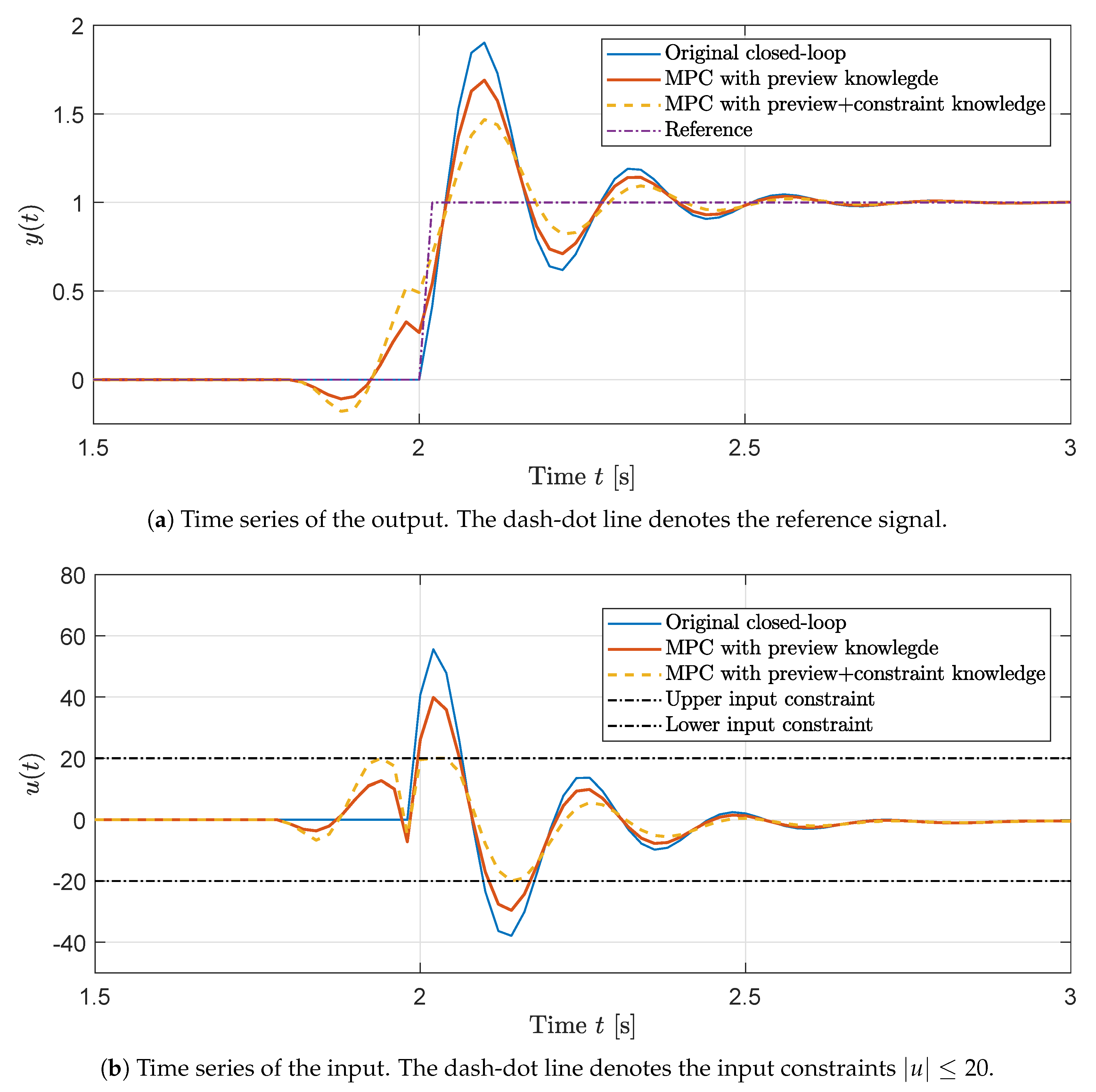
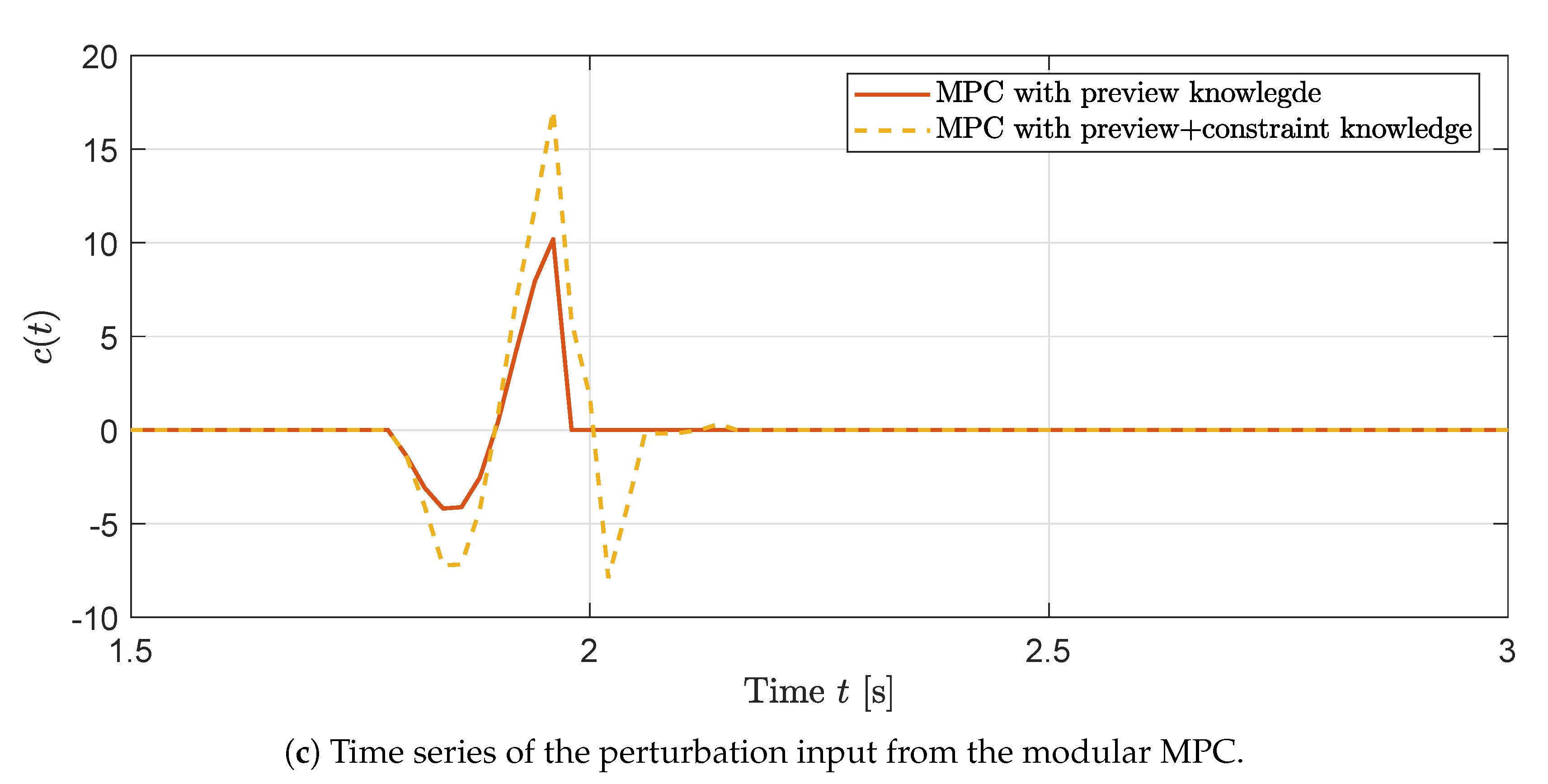
The control task is to track a step reference signal that happens at 2 s. Figure 2a shows that with the preview knowledge, the proposed modular MPC (the thick solid red line) clearly achieved better tracking with less overshoot than the system with only the original controller (the thin solid blue line). The input effort was also lower when the MPC module anticipated the changes in the preview measurement, as shown in Figure 2b. Furthermore, the perturbation input from the modular MPC is illustrated in Figure 2c. It is clearly shown that the modular MPC is only active between 1.8 s and 2.2 s, where, with the preview horizon $n_a=10$ (that is 0.2 s), the MPC module noticed a sudden step changes from the preview reference signal and provided additional perturbation input to the closed-loop system for improving the overshoot.

4.2. Example 2: Handling Preview and Constraint Information

This example shows how the constraint handling feature is incorporated into the existing controller. The control task is equivalent to the previous example that a step reference is tracked, but, in this example, a constraint is imposed on the input as $\left|u\right|\le 20$. Figure 2a,b show the output and input of the original closed-loop system and the modular MPC algorithm with preview and constraint information. In Figure 2a, it is clearly demonstrated that the modular MPC with constraint and preview knowledge (the dashed line) drove the output into the more opposite direction at the beginning (around 1.85 s), as comparing to the MPC layer with only the preview measurement (the thick solid red line). Figure 2b shows how the modular MPC with constraint and preview knowledge (the dashed line) anticipated constraint violation and reacted more aggressively in advance, in comparison to the MPC algorithm with only the preview knowledge (the thick solid red line). In addition, in Figure 2c, it reveals that, when the constraint violation was not expected and the preview signal reached a steady-state, the perturbation input from the modular MPC always remained at zero.

4.3. Optimality and Consistency in Predictions

Section 4.1 and Section 4.2 showed that the preview action from the modular MPC solely handled the transient of the closed-loop dynamics in the unconstrained case. To demonstrate that the preview action is optimal, consistency in predictions is examined, as suggested by Remark 2. Figure 3 shows the predicted sequences and closed-loop trajectory of the perturbation input at different time instant. At each time instant, the modular MPC predicted the perturbation input sequence (grey solid line) and the first sample of the sequence (star) was then implemented into the system. By inspecting Figure 3, the predictions are consistent with the actual closed-loop input trajectory (dash line). In other words, the tail of the predictions at the previous time sample is included in the predictions at the later time. Thus, the preview control action is optimal with respect to the overall closed-loop behaviour.

5. Conclusions

This paper has first revisited the modular MPC design where the preview measurements and constraint handling capability are retrofitted into a known output-feedback controller, together with the conditions to ensure the former does not interfere with the closed-loop dynamics provided by the latter. Based upon the modular MPC design, this paper has proposed a preview compensator design procedure within the modular MPC formulation. The key conditions were derived to ensure that the preview compensator is systematic and well-designed, in the sense that the preview control action only handles the transient of the existing closed-loop and once the steady-state is reached, the input from the preview compensator remains at zero. Two key benefits of the modular MPC design were discussed, namely: (i) the sensitivities and robustness properties of the nominal output-feedback controller are retained in the unconstrained case and such robust properties are, to some extent, extended to the constrained case; and, (ii) the preview control with constraint handling can be systematically incorporated into the existing feedback controller without replacing it. Numerical simulation studies have been provided in order to illustrate the efficacy of the modular MPC design.

References

1. Clarke, D.; Mohtadi, C.; Tuffs, P. Generalized predictive control—Part I. The basic algorithm. Automatica 1987, 23, 137–148. [Google Scholar] [CrossRef]
2. Limon, D.; Alvarado, I.; Alamo, T.; Camacho, E. MPC for tracking piecewise constant references for constrained linear systems. Automatica 2008, 44, 2382–2387. [Google Scholar] [CrossRef]
3. Ferramosca, A.; Limon, D.; Alvarado, I.; Alamo, T.; Camacho, E.F. MPC for tracking with optimal closed-loop performance. Automatica 2009, 45, 1975–1978. [Google Scholar] [CrossRef]
4. Carrasco, D.S.; Goodwin, G.C. Feedforward model predictive control. Annu. Rev. Control 2011, 35, 199–206. [Google Scholar] [CrossRef]
5. Valencia-Palomo, G.; Rossiter, J.A.; López-Estrada, F.R. Improving the feed-forward compensator in predictive control for setpoint tracking. ISA Trans. 2014, 53, 755–766. [Google Scholar] [CrossRef]
6. Mirzaei, M.; Hansen, M.H. A LIDAR-assisted model predictive controller added on a traditional wind turbine controller. In Proceedings of the 2016 American Control Conference (ACC), Boston, MA, USA, 6–8 July 2016; pp. 1381–1386. [Google Scholar]
7. Garone, E.; Di Cairano, S.; Kolmanovsky, I. Reference and command governors for systems with constraints: A survey on theory and applications. Automatica 2017, 75, 306–328. [Google Scholar] [CrossRef] [Green Version]
8. Gilbert, E.G.; Ong, C.J. Constrained linear systems with hard constraints and disturbances: An extended command governor with large domain of attraction. Automatica 2011, 47, 334–340. [Google Scholar] [CrossRef]
9. Borrelli, F.; Falcone, P.; Pekar, J.; Stewart, G. Reference governor for constrained piecewise affine systems. J. Process Control 2009, 19, 1229–1237. [Google Scholar] [CrossRef]
10. Rossiter, J.A.; Kouvaritakis, B. Reference governors and predictive control. In Proceedings of the American Control Conference, Philadelphia, PA, USA, 24–26 June 1998; Volume 6, pp. 3692–3693. [Google Scholar]
11. Aghaei, S.; Sheikholeslam, F.; Farina, M.; Scattolini, R. An MPC-based reference governor approach for offset-free control of constrained linear systems. Int. J. Control 2013, 86, 1534–1539. [Google Scholar] [CrossRef]
12. Klauco, M. MPC-based Reference Governors: Theory and Applications. Ph.D. Thesis, Slovak University of Technology in Bratislava, Bratislava, Slovakia, 2017. [Google Scholar]
13. Lio, W.H.; Rossiter, J.A.; Jones, B.L. Predictive control design on an embedded robust output-feedback compensator for wind turbine blade-pitch preview control. In Proceedings of the 2016 European Control Conference, Aalborg, Denmark, 29 June–1 July 2016. [Google Scholar]
14. Lio, W.H.; Jones, B.L.; Rossiter, J.A. Preview predictive control layer design based upon known wind turbine blade-pitch controllers. Wind Energy 2017, 20, 1207–1226. [Google Scholar] [CrossRef]
15. Rossiter, J.A.; Grinnell, B.G. Improving the tracking of generalized predictive control controllers. Proc. Inst. Mech. Eng. Part I J. Syst. Control. Eng. 1996, 210, 169–182. [Google Scholar] [CrossRef]
16. Rossiter, J.A.; Valencia-Palomo, G. Feed forward design in MPC. In Proceedings of the European Control Conference, Budapest, Hungary, 23–26 August 2009. [Google Scholar]
17. Muske, K.R.; Rawlings, J.B. Model predictive control with linear models. AIChE J. 1993, 39, 262–287. [Google Scholar] [CrossRef]
18. Rossiter, J.A.; Kouvaritakis, B.; Rice, M.J. A numerically robust state-space approach to stable-predictive control strategies. Automatica 1998, 34, 65–73. [Google Scholar] [CrossRef]
19. Rossiter, J.A. Model-Based Predictive Control: A Practical Approach; CRC Press: Boca Raton, FL, USA, 2003. [Google Scholar]
20. Kouvaritakis, B.; Rossiter, J.A.; Schuurmans, J. Efficient robust predictive control. IEEE Trans. Autom. Control 2000, 45, 1545–1549. [Google Scholar] [CrossRef]
21. Gilbert, E.; Tan, K. Linear systems with state and control constraints: The theory and application of maximal output admissible sets. IEEE Trans. Autom. Control 1991, 36, 1008–1020. [Google Scholar] [CrossRef]
22. Pluymers, B.; Rossiter, J.; Suykens, J.; De Moor, B. The efficient computation of polyhedral invariant sets for linear systems with polytopic uncertainty. In Proceedings of the 2005, American Control Conference, Portland, OR, USA, 8–10 June 2005; pp. 804–809. [Google Scholar]
23. Kouvaritakis, B.; Cannon, M. Model Predictive Control: Classical, Robust and Stochastic; Advanced Textbooks in Control and Signal Processing; Springer International Publishing: Cham, Switzerland, 2016. [Google Scholar]
24. Kreindler, E.; Jameson, A. Optimality of linear control systems. IEEE Trans. Autom. Control 1972, 17, 349–351. [Google Scholar] [CrossRef]
25. Boyd, S.; El Ghaoui, L.; Feron, E.; Balakrishnan, V. Linear Matrix Inequalities in System and Control Theory; Society for Industrial and Applied Mathematics: Philadelphia, PA, USA, 1994. [Google Scholar]
26. Di Cairano, S.; Bemporad, A. Model Predictive Control Tuning by Controller Matching. IEEE Trans. Autom. Control 2010, 55, 185–190. [Google Scholar] [CrossRef]
27. Hartley, E.N.; MacIejowski, J.M. Designing output-feedback predictive controllers by reverse-engineering existing LTI controllers. IEEE Trans. Autom. Control 2013, 58, 2934–2939. [Google Scholar] [CrossRef] [Green Version]
28. Maciejowski, J. Predictive Control with Constraints; Prentice Hall: Upper Saddle River, NJ, USA, 2000. [Google Scholar]
29. Kothare, M.V.; Balakrishnan, V.; Morari, M. Robust constrained model predictive control using linear matrix inequalities. Automatica 1996, 32, 1361–1379. [Google Scholar] [CrossRef] [Green Version]
30. Raković, S.; Mayne, D. A simple tube controller for efficient robust model predictive control of constrained linear discrete time systems subject to bounded disturbances. IFAC Proc. Vol. 2005, 38, 241–246. [Google Scholar] [CrossRef] [Green Version]
31. Scokaert, P.O.M.; Rawlings, J.B. Feasibility issues in linear model predictive control. AIChE J. 1999, 45, 1649–1659. [Google Scholar] [CrossRef]
32. Zeilinger, M.N.; Morari, M.; Jones, C.N. Soft Constrained Model Predictive Control With Robust Stability Guarantees. IEEE Trans. Autom. Control 2014, 59, 1190–1202. [Google Scholar] [CrossRef]
33. Rawlings, J.B.; Bonné, D.; Jørgensen, J.B.; Venkat, A.N.; Jørgensen, S.B. Unreachable Setpoints in Model Predictive Control. IEEE Trans. Autom. Control 2008, 53, 2135–2141. [Google Scholar] [CrossRef]
34. Shead, L.R.E.; Muske, K.R.; Rossiter, J.A. Conditions for which linear MPC converges to the correct target. J. Process Control 2010, 20, 1243–1251. [Google Scholar] [CrossRef]
35. Aström, K.J.; Murray, R.M. Feedback Systems: An Introduction for Scientists and Engineers; Princeton University Press: Princeton, NJ, USA, 2010. [Google Scholar]
Figure 1. Schematic of modular model predictive control layer on top of an existing feedback controller.
Processes 08 00855 g001
Figure 2. Time series of the output, input, and perturbation input trajectories. The thin solid (blue) lines denote the original closed-loop with the existing controller. The thick (red) solid lines represent the response of the closed-loop with the modular MPC with the preview measurement, whilst the dashed lines denote the original closed-loop with the proposed MPC module with the preview and constraint knowledge.
Processes 08 00855 g002aProcesses 08 00855 g002b
Figure 3. Time-series of predictions and closed-loop trajectory of the perturbation input. Four diagrams at a different time, showing that the predicted perturbation sequence (grey solid line) is consistent with the actual input trajectory (dash line).
Processes 08 00855 g003