Nanofluid Flow Past a Stretching Plate

Abstract

Viscous nanofluid flow due to a sheet moving with constant speed in an otherwise quiescent medium is studied for three types of nanofluids, such as alumina (Al₂O₃), titania (TiO₂), and magnetite (Fe₃O₄), in a base fluid of water. The heat and mass transfer characteristics are investigated theoretically using the boundary layer theory and numerically with computational fluid dynamics (CFD) simulation. The velocity, temperature, skin friction coefficient, and local Nusselt number are determined. The obtained results are in good agreement with known results from the literature. It is found that the obtained results for skin friction and for the Nusselt number are slightly greater than those obtained via boundary layer theory.

1. Introduction

The development of boundary layer theory was initiated by Ludwig Prandtl [1] in the early 1900s, and many world-renowned scientists, including Blasius [2], have worked on further development. The name of the boundary layer comes from Prandtl, and in this layer we find a significant change in velocity, such as a layer close to the surface of a solid body. However, there is another type of boundary layer, and in addition to the change in velocity, a thermal boundary layer can also be defined based on the change in temperature. Prandtl’s theory led to the conclusion that the losses of fluid flowing in a pipe or duct occur almost entirely in the usually very thin boundary layer adhering to the wall. The analytical solution to the boundary layer problem comes from Blasius introducing the similarity method [3].

Prandtl’s boundary layer theory is applied to many practical engineering problems to predict skin friction drag. In metallurgical, petrochemical, and plastics processing applications, boundary layer theory is very important. The surface-driven flow in a resting fluid plays an important role in many material processing processes, e.g., hot rolling, metalworking, and continuous casting (see [4,5,6]). The flow of the boundary layer of a plane moving at a uniform velocity in Newtonian fluid was investigated analytically by Sakiadis [7]. His results were experimentally verified by Tsou et al. [8]. The continuous extrusion of polymer sheets from a die to the winding cylinder was investigated. The slit and the winding cylinder are placed at a finite distance from each other. Sakiadis assumed that a steady state would develop after a certain time after the start of the process. Tsou et al. [8] showed in their studies containing both analytical and experimental results that the laminar velocity field determined with the analytical solution for Newtonian fluid show a very good agreement with the measured data.

The Sakiadis problem of fluid flow along sheet surfaces has been extended in many ways in recent decades. In the case of linear stretching, Crane [9] provided a solution to Sakiadis’ problem for heat and mass transfer in a closed form with exponential function. Chakrabarti and Gupta investigated flow characteristics over a linearly stretched surface through a transverse magnetic field [10]. When the surface is stretched nonlinearly, Banks investigated the governing boundary layer equations [11]. The flow characteristics of non-Newtonian power law-type fluids over a stretched sheet was investigated by Bognár et al. [12,13,14]. Haider et al. [15] analysed magnetohydrodynamic viscous fluid flow due to exponentially stretching sheet with the homotopy analysis method. In [16], Mahabaleshwar examines the flow properties of fluid flow through porous media for a variety of boundary conditions. Among the different rheological models, the Walters-B fluid model is applied for description of the complex flow behaviour of various polymer solutions. Andersson investigated the Walters-B flow characteristics along a linearly stretching surface [17]. In [18], Walters-B Sakiadis boundary layer flow is solved by Tonekaboni et al. An incompressible and electrically conducting isothermal viscoelastic Walters-B fluid flow due to a stretching surface with quadratic velocity was studied by Siddheshwar [19]. The boundary layer equations through a porous medium over a stretching plate with superlinear stretching velocity were investigated by Singh et al. [20]. The influence of variable viscosity is analysed in heat and mass transfer properties in [21,22,23,24].

Recently, in the literature, the nanofluid flows have been of great interest. Nanofluids are smart solutions in heat exchangers applied in many industrial applications responsible for the transfer of heat between fluids and device surfaces. Their applications include air conditioning systems, nuclear reactors, solar film collectors, etc.First, Choi [25] introduced the term of nanofluids. The purpose of adding nano-sized solid particles to the base fluid, e.g., metals, metal oxides, and ceramics, is to enhance thermal the conductivity of base fluids. It is known that by combining a very small number of nanoparticles to traditional base fluids, the thermal conductivity can be increased up to two times [26,27,28]. Mathematical modelling of nanofluids is integrated as single-phase model or a two-phase model into the description of the flow, for the governing equations.Raza et al. [29] investigated the effect of temperature-dependent thermal conductivity on Williamson nanofluid flow in a nonlinearly stretching, variable-thickness plate in the presence of magnetic field. The magnetohydrodynamic stagnation point flow for nanofluids past a stretching surface with melting heat transfer was studied by Ibrahim [30].

Ahmad et al. [31] and Bachok et al. [32] tested the effect of solid nanoparticle concentration for the Blasius and Sakiadis problems by investigating Cu, Al₂O₃, and TiO₂. Gingold [33] pointed out that due to the simplifications applied in boundary layer theory, we only get approximate values for flow characteristics. Experimental results published by Liepmann [34] and Schlichting [3] for fluid flow over a flat surface showed lower velocity values in the neighbourhood of the surface compared to the solution obtained using the boundary layer theory. The experiments of Janour [35], Schaaf, and Sherman [36] resulted in a higher skin friction drag in the range 0–1000 of the Reynolds number than in the theoretical Blasius solution.

The researchers have found that microfluidic flow could be used to grow defect-free crystals, as demonstrated in the papers [37,38]. Recently, several authors have shown their keen interest in the heat and mass transfer phenomena of nanofluid flow over stretching sheet (see [39,40,41,42,43]).

Following the investigations in [31,32], our aim is to present an analysis for the flow and heat transfer characteristics of a continuously moving flat plate in a nanofluid. The problem is solved using computational fluid dynamics (CFD), as well as analytically with the similarity approach, for three types of nanofluids of nanoparticles, namely alumina (Al₂O₃), titania (TiO₂), and magnetite (Fe₃O₄), with water as the base fluid. The main interest is to show the influence of the concentration on the fluid characteristics, and to compare the velocity and temperature distribution, the skin friction, and Nusselt number obtained with the two solution techniques.

2. Mathematical Formulation

Consider a two-dimensional laminar boundary layer flow over a continuously moving, flat surface for a water-based nanofluid containing three different types of nanoparticles. The thermophysical properties of the nanofluids are given in

Table 1. The thermophysical properties of water, as well as Al₂O₃, TiO₂, and Fe₃O₄ particles.

Parameter	Fe3O4	TiO2	Al2O3	H2O
$\rho \left(\mathrm{kg}/{\mathrm{m}}^3\right)$	5180	4250	3970	997.1
$C_p (\mathrm{J}/\mathrm{kg}·\mathrm{K}$)	670	686.2	765	4179
$k \left(\mathrm{W}/\mathrm{m}·\mathrm{K}\right)$	9.7	8.9538	40	0.613
$\mathsf{\mu }\left(\mathrm{Pa}·\mathrm{s}\right)$	—	—	—	0.001

[44]. The shape of the nanoparticles is spherical, and the average particle size is considered to be 20 nm. It is assumed that the nanofluid is incompressible, the flow is laminar, and the effect of viscous distribution and radiation is negligible.

In the Cartesian coordinate system, the $x$-axis is chosen along the flow direction, while the $y$-axis is perpendicular to the surface. The nanofluid is confined above the horizontal surface, which coincides with the positive $x$-axis. The ambient fluid has a constant temperature $T_{\infty }$, and the temperature of the surface is $T_w$. In our case $T_w$ < $T_{\infty }$. The velocity components $u$ and $v$ are the parallel and normal velocity components to the plate, respectively; ${\mu }_{nf}$ denotes the dynamic viscosity, ${\rho }_{nf}$ is the density, and ${\alpha }_{nf}$ is the thermal diffusivity of the nanofluid.

Using these assumptions and notations, the continuity, momentum, and energy equations in the vectoral form for the steady flow can be formulated as follows:

$$\nabla .\overrightarrow{V}=0,$$

(1)

$$\left(\overrightarrow{V}.\nabla \right)\overrightarrow{V}=-\frac{1}{{\rho }_{nf}}\nabla p+\frac{{\mu }_{nf}}{{\rho }_{nf}}{\nabla }^2\overrightarrow{V},$$

(2)

$$\left(\overrightarrow{V}.\nabla \right)T={\alpha }_{nf}{\nabla }^{2}T,$$

(3)

where the following notations are used: $\overrightarrow{V}$ is the velocity vector, $T$ is the temperature of the nanofluid, and $p$ is the pressure of the nanofluid.

In the traditional boundary layer theory, many assumptions are made: the momentum and thermal boundary layer are very thin, compared with the flow’s length scale, and grow in the direction of motion of the surface; the velocity parallel to the wall is much larger than the velocity components ($v$); and the derivatives of the velocity components to the wall are large [33]. The part of the liquid flow that is outside the thermal boundary layer is not affected by the heat transfer of the moving surface. Under these approximations, Equations (1)–(3) are written in the following forms:

$$\frac{\partial u}{\partial x}+\frac{\partial v}{\partial y}=0$$

(4)

$$u\frac{\partial u}{\partial x}+v\frac{\partial u}{\partial y}=\frac{{\mu }_{nf}}{{\rho }_{nf}}\frac{{\partial }^{2}u}{\partial y^2}$$

(5)

$$u\frac{\partial T}{\partial x}+v\frac{\partial T}{\partial y}={\alpha }_{nf}\frac{{\partial }^{2}T}{\partial y^2}.$$

(6)

The flow of nanofluid in an otherwise quiescent medium along a plate moving at a constant speed $U$ is examined. Conventional impermeability and anti-slip are applied to the solid surface, and in addition to the viscous boundary layer, the flow rate component $u=0$. The boundary conditions for the velocity and temperature fields for the Sakiadis flow problem are

$$u\left(x,0\right)=U,v\left(x,0\right)=0,T\left(x,0\right)=T_w,\underset{y\to \infty }{lim}u\left(x,y\right)=0,\underset{y\to \infty }{lim}T\left(x,y\right)=T_{\infty }$$

(7)

For the thermophysical properties of the nanoparticle-water nanofluid, the following formulas are defined for the effective density:

$${\rho }_{nf}=\left(1-\varphi \right){\rho }_b+\varphi {\rho }_p$$

(8)

where ${\rho }_b$and ${\rho }_p$ denote the density base fluid and nanoparticles, respectively, and $\varphi$denotes nanoparticle volume fraction; for the effective viscosity

$${\mu }_{nf}=\frac{{\mu }_b}{{(1-\varphi )}^{2.5}}$$

(9)

where ${\mu }_{nf}$ is the viscosity of the nanofluid and ${\mu }_b$ is the viscosity of the base fluid; for the effective heat capacity

$${(\rho C_p)}_{nf}=\varphi {(\rho C_p)}_p+\left(1-\varphi \right){(\rho C_p)}_b$$

(10)

and for the effective thermal conductivity

$$k_{nf}=k_b\frac{k_p+2k_b-2\varphi \left(k_b-k_p\right)}{k_p+2k_b+\varphi \left(k_b-k_p\right)}$$

(11)

where $k_{nf}$ denotes the thermal conductivity of nanofluid, $k_b$ the thermal conductivity of base fluid, and $k_p$ the thermal conductivity of the particles.

The Sakiadis problem has been reported in the physical and mathematical literature, and this has again aroused interest in the analytical and numerical study of boundary layers. By analogy with the Sakiadis description, we studied the similarity solutions and the CFD simulation results to investigate the heat and mass properties, comparing the obtained results and giving numerical justification of the Blasius boundary layer approach.

3. Results Using Similarity Method and Discussion

Let us now introduce the stream function $\psi$ as

$$u=\frac{\partial \psi }{\partial y}, v=-\frac{\partial \psi }{\partial x}$$

(12)

Applying similarity transformations with the dimensionless similarity variable

$$\eta ={\left(\frac{U}{{\nu }_{nf}x}\right)}^{\raisebox{1ex}{$1$}\!\left/ \!\raisebox{-1ex}{$2$}\right.}y$$

(13)

the stream function and the non-dimensional temperature are expressed as

$$\psi ={\left(U{\nu }_{nf}x\right)}^{\raisebox{1ex}{$1$}\!\left/ \!\raisebox{-1ex}{$2$}\right.}f\left(\eta \right),\theta \left(\eta \right)=\frac{T-T_{\infty }}{T_w-T_{\infty }}$$

(14)

where ${\mathsf{\nu }}_{nf}=\frac{{\mathsf{\mu }}_{nf}}{{\mathsf{\rho }}_{nf}}$ denotes the kinematic viscosity.

Taking the substitution (12), the continuity Equation (4) is automatically satisfied. The momentum Equation (5) and the thermal energy Equation (6) are transformed into a set of ordinary differential equations. From Equations (5) and (6), we obtain a system of ordinary differential equations for $f$and $\theta$, as follows:

$$\frac{{\rho }_b}{{\rho }_{nf}}\frac{{\mu }_{nf}}{{\mu }_b}f‴+\frac{1}{2}ff″=0$$

(15)

$${\alpha }_{nf}\frac{{\rho }_b}{{\mu }_b}\theta ″+\frac{1}{2}f\theta \prime =0$$

(16)

Where the prime denotes the differentiation with respect to $\eta$. Under conditions (7), these equations are considered together with the following boundary conditions:

$$f\left(0\right)=0,f\prime \left(0\right)=1,\underset{\eta \to \infty }{lim}f\prime \left(\eta \right)=0,$$

(17)

$$\theta \left(0\right)=1,\underset{\eta \to \infty }{lim}\theta \left(\eta \right)=0$$

(18)

The dimensional velocity components can be given with the similarity function $f$ as

$$u\left(x,y\right)=Uf\prime \left(\eta \right)$$

(19)

$$v\left(x,y\right)=v^{*}\left(x\right)\left[\eta f\prime \left(\eta \right)-f\left(\eta \right)\right]$$

(20)

where $v^{*}\left(x\right)=\frac{1}{2}UR{e}_x{}^{-\frac{1}{2}}$, and the local Reynolds number $R{e}_x$ is defined by ${Re}_x=Ux/{\nu }_{nf}$. The dimensional temperature is obtained as

$$T\left(x,y\right)=T_{\infty }+\left(T_w-T_{\infty }\right)\theta \left(\eta \right).$$

(21)

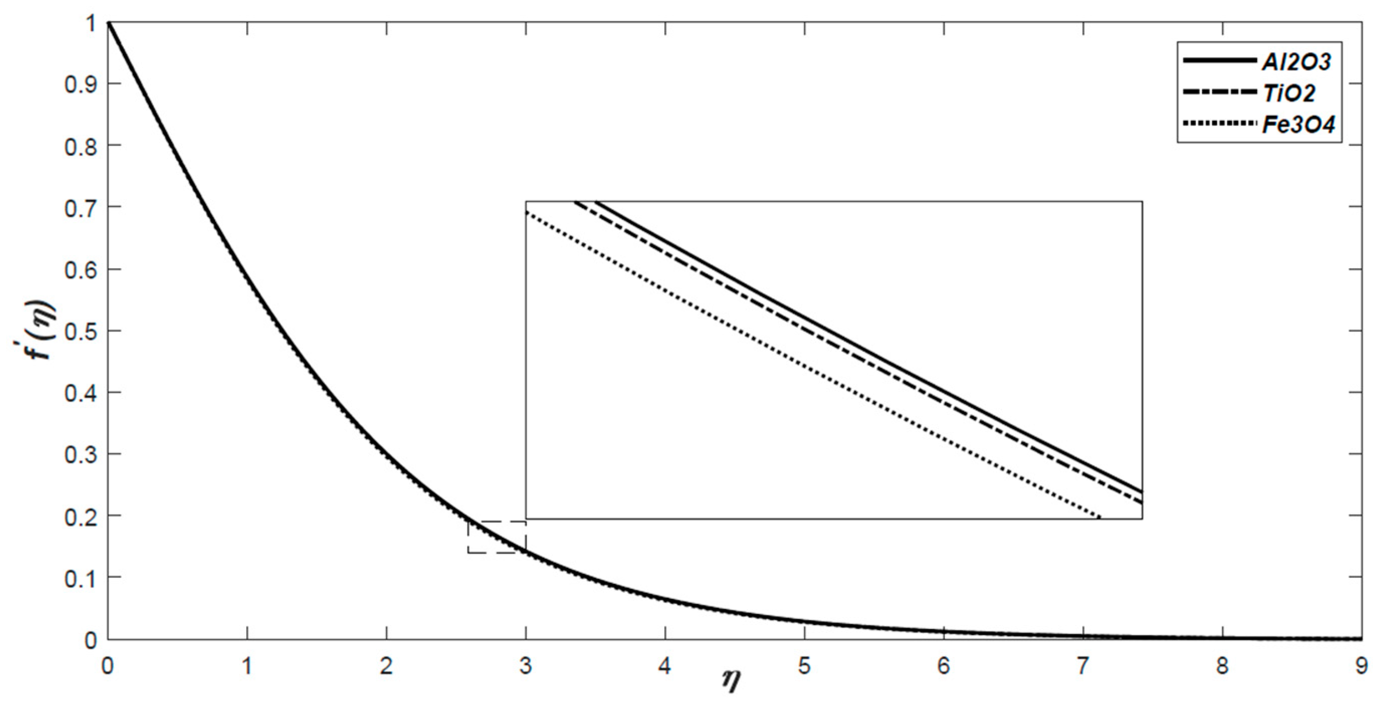
Using the fourth-order method (bvp4c) in MATLAB, the system (15) and (16) is solved with conditions (17) and (18), when the nanofluid properties are calculated according to formulas (8)–(11) using the thermophysical values given in Table 1 for Al₂O₃, TiO₂, and Fe₃O₄ particles, as well as the base fluid of suspension water. Our aim was to investigate the impacts of the volume fraction and nanoparticle’s material type on the heat and mass transfer characteristics.

Figure 1 exhibits the dimensionless velocity distributions for all three nanofluids for 2% additives in the base fluid. It shows that the velocity is greater for Al₂O₃ than for the other two materials. Figure 2 represents the temperature distribution for the same cases. Here, the Al₂O₃ also shows greater values than the others.

The effect of the volume fraction $\varphi$ is depicted in Figure 3 and Figure 4. It was observed that increasing $\varphi$ will slow down the fluid flow velocity and will increase the non-dimensional temperature.

The skin friction coefficient and the local Nusselt number is of engineering interest, and these will be presented and discussed in detail. The wall shear stress (${\tau }_w$) and heat flux ($q_w$) are defined as

$${\tau }_w={\mu }_{nf}{\left(\frac{\partial u}{\partial y}\right)}_{y=0},\hspace{1em}\hspace{1em}{q}_w=-k_{nf}{\left(\frac{\partial T}{\partial y}\right)}_{y=0}$$

(22)

while the skin friction coefficient ($C_f$) and the local Nusselt number ($Nu$) are defined as

$$C_f=\frac{{\tau }_w}{{\rho }_b{U}^2},\hspace{1em}\hspace{1em}Nu=\frac{x{q}_w}{k_{nf}\left(T_w-T_{nf}\right)}.$$

(23)

Applying the similarity variables defined in (8) and (9), one gets

$$R{e}_x^{1/2}{C}_f=\frac{1}{{\left(1-\varphi \right)}^{2.5}}{f}^{″}\left(0\right),\hspace{1em}\hspace{1em}R{e}_x^{-1/2}Nu=-\frac{k_{nf}}{k_b}{\theta }^{\prime }\left(0\right),$$

(24)

where the local Reynolds number $R{e}_x$ is defined by ${\mathrm{Re}}_x=\frac{{\rho }_{nf}Ux}{{\mu }_{nf}}$.

4. Results with CFD Simulations and Discussion

Nowadays, the computation fluid dynamics (CFD) simulation has become an effective tool to predict results in fluid flow characteristics.

The CFD simulations have been performed for the laminar nanofluid flow, according to Figure 5, and Equations (1)–(3) were discretized and solved using ANSYS 18. The sheet was maintained at a constant temperature $T_w$ = 400 K. The fluid flows with constant velocity $U=0.01 \mathrm{m}/\mathrm{s}$and the temperature outside the thermal boundary layer was $T_{\infty }$ = 300 K. The length of the plate was $L=1 \mathrm{m}$. For the computational domain and mesh, the computational domain geometry was generated using Design Modeler, and the grid was generated using ANSYS Fluent mesh. The CFD domain consists of inlet and outlet, which had been divided by the number of division type with 100 divisions; the behaviour was set to hard, with bias factor 40, in order to increase the number of subdomains near to the plate and increase the preciseness near the wall. The boundary conditions had been set up as follows: side AD is symmetry, BC is the wall, AB is the velocity inlet, and CD is the outlet. Both AD and BC were divided using the same method, with 200 divisions. A laminar model was used with pressure–velocity coupling. The relaxation factor was 1 for density; body force and energy, the thermophysical properties of nanofluids (including density, thermal conductivity, viscosity, and thermal capacity) were calculated using a single-phase approach. In order to check grid sensitivity, the local Nusselt number was evaluated. A comprehensive mesh sensitivity study had been done to minimize the numerical influences introduced by the size of the meshes. The analysis of the mesh sensitivity had been done for five meshes (with the number of cells being 7000, 9600, 14,400, 20,000, and 26,400), and the Nusselt number on the plate for each mesh had been compared. It was noticed that the Nusselt number for the mesh with 20,000 cells was found to be satisfactory to ensure the accuracy (${10}^{-6})$ of the solution, as well as the independency of the grid, which was applied in the further simulations.

Applying Equations (8)–(11), the effect of volume concentration on the density, viscosity, thermal capacity, and thermal conductivity were determined in [45] for the three nanofluids, with data given in Table 1. It was found that the density and the viscosity increase with $\varphi$; however, the thermal capacity and thermal conductivity have opposite behaviour.

Figure 6 and Figure 7 show the impact of the nanoparticles’ material on the dimensional velocity and temperature profiles for $\varphi =0.02$, respectively. We remark that these figures are in correlation with Figure 1 and Figure 2.

The impact of the nanoparticle’s concentration was investigated on Al₂O₃–water nanofluid in Figure 8 and Figure 9. It follows, according to Figure 3 and Figure 4, that more additives will reduce the velocity and increase the velocity.

The skin friction coefficient and the local Nusselt number were analysed using CFD simulations. Figure 10 exhibits the impact of the nanoparticle’s material on $C_f$ for $\varphi =0.02$ along the flat surface. We found that the skin friction is higher Fe₃O₄ than for Al₂O₃ and TiO₂.

The skin friction coefficient variation with the Reynolds number is shown in Figure 11 for Al₂O₃ in the range of the corresponding Reynolds number. We can observe that the larger $\varphi$ is, the larger $C_f$ is.

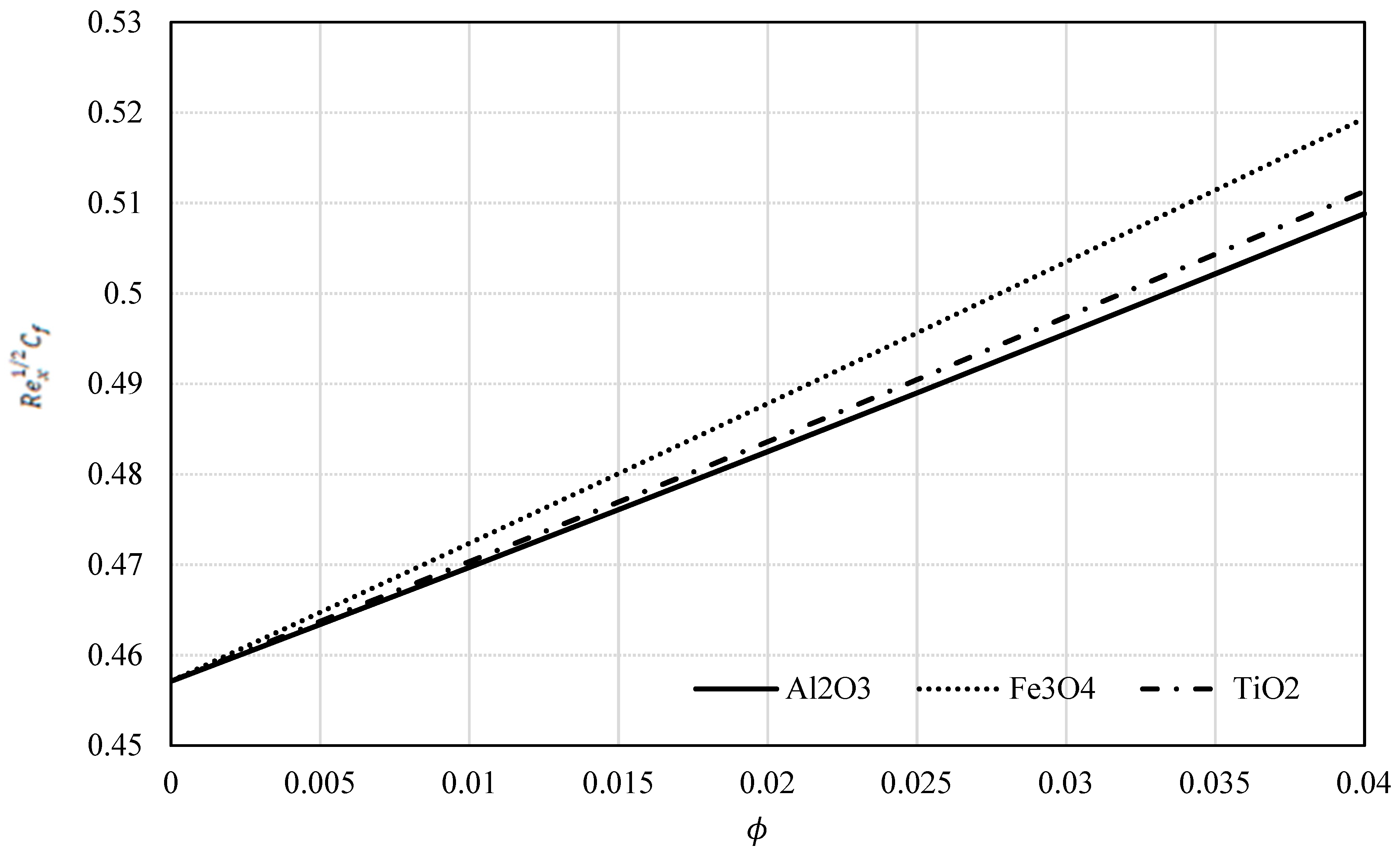
The effect of the nanoparticle’s material on skin friction is examined in Figure 12, in the range 0.00–0.04. It was concluded that the highest values were obtained for Fe₃O₄, while the lowest were for Al₂O₃.

In Figure 13, the values of $R{e}_x^{1/2}{C}_f$versus $\varphi$ are exhibited for all three additive materials. We remark that the same trends can be seen as in Figure 12.

Figure 14 depicts the variation of the Nusselt number along the sheet surface. One can see a slight difference along the x-axis for all three nanofluids when $\varphi =0.02$. The bigger values for Nu were obtained for Al₂O₃.

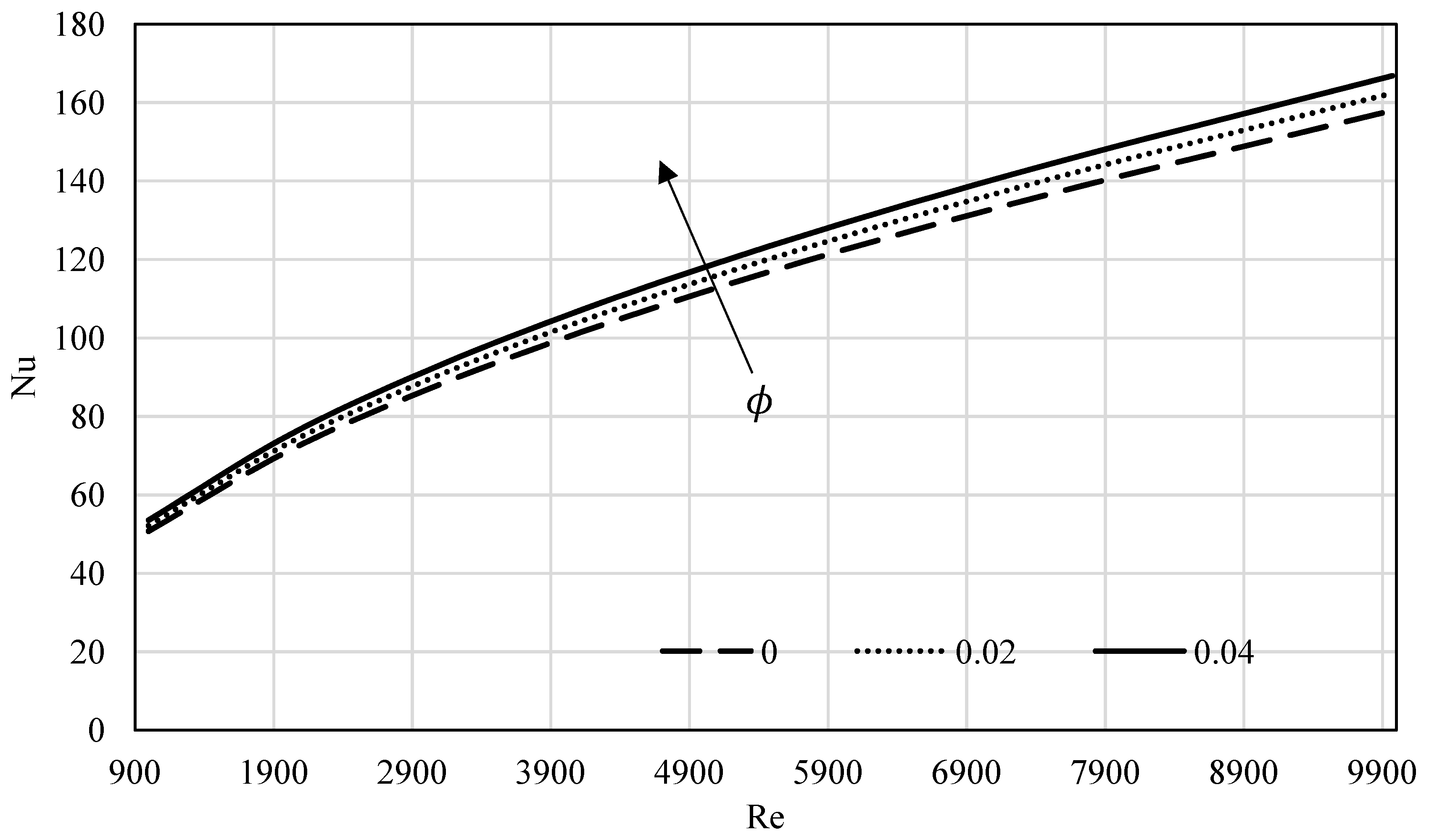
The influence of the volume fraction on the local Nusselt number is investigated in Figure 15 for Al₂O₃ in the range of Reynolds number 900–9000. It can be seen from the figure that the increase in ϕ will induce an increase in the Nusselt number as well.

In Figure 16, the effect of the nanomaterial on the local Nusselt number is investigated. As the volume fraction increases, the local number of Nusselt number increases. However, the biggest values are obtained for Al₂O₃.

Figure 17 reveals the impact of the nanoparticle’s material on $R{e}_x^{-1/2}Nu.$ We can observe the same trends in Figure 17 as in Figure 16.

Table 2. Variation of $R{e}_x^{1/2}{C}_f$ with $\varphi$.

$\mathit{\varphi }$	Al2O3		TiO2		Fe3O4
	Similarity	CFD	Similarity	CFD	Similarity	CFD
0.00	0.44455	0.45712	0.44455	0.45712	0.44455	0.45712
0.01	0.45682	0.46971	0.45743	0.47035	0.45947	0.47238
0.02	0.46929	0.48252	0.47052	0.48361	0.47458	0.48783
0.03	0.48198	0.49556	0.48382	0.49741	0.48988	0.50349
0.04	0.49490	0.50883	0.49735	0.51129	0.50540	0.51938

and

Table 3. Variation of $R{e}_x^{-1/2}Nu$ with $\varphi$.

$\mathit{\varphi }$	Al2O3		TiO2		Fe3O4
	Similarity	CFD	Similarity	CFD	Similarity	CFD
0.00	1.36704	1.58199	1.36704	1.58199	1.36704	1.58199
0.01	1.38267	1.60408	1.37974	1.60056	1.38043	1.60221
0.02	1.39833	1.62624	1.39426	1.61913	1.39387	1.62240
0.03	1.41401	1.64942	1.40520	1.63766	1.40737	1.64264
0.04	1.42975	1.67068	1.41798	1.65624	1.42093	1.66293

show the comparison of $R{e}_x^{1/2}{C}_f$ and $R{e}_x^{-1/2}Nu$, respectively. These values are determined by the similarity solutions with $f″\left(0\right)$ and ${\theta }^{\prime }\left(0\right)$, using the equations in (24) and with CFD simulations as well. We remark that in the range 0.00–0.02 for $\varphi$, the values obtained with CFD are slightly greater for both quantities than for the analytical solution obtained with the similarity method. However, the difference is small, less than 14.5%, and is especially small (2.7%) for $R{e}_x^{1/2}{C}_f$ The difference is due to boundary layer approximations. We consider that the CFD simulation results could be closer to the experimental results.

5. Conclusions

The Sakiadis flow was investigated by determining the velocity and temperature in three types of nanofluids along a continuously moving sheet surface. The skin friction coefficient and the local Nusselt number were calculated. Two methods were used: one of them was analytically applying the traditional Blasius’ similarity transformation, and solving the obtained coupled ordinary differential equations; the other solution was obtained using CFD simulations. We found that the solid volume fraction significantly influences the fluid flow and heat transfer properties. Comparing the three nanoparticles’ materials, we note that the Al₂O₃ has significantly greater thermal conductivity. The larger velocity and temperature values are obtained in the boundary layer for alumina–water fluid than for the other two nanomaterials. Increasing the concentration of nanomaterial has produced a decrease in velocity and an increase in temperature in the momentum and thermal boundary layers, respectively. The skin friction decreases and the Nusselt number increases with the Reynolds number. The values of $C_f$ and Nu are depicted with the nanoparticle concentration. It was concluded that both linearly increase with $\varphi$ (see Figure 12 and Figure 16). For Al₂O₃, the values of the skin friction coefficient are smaller than for titania (TiO₂) and magnetite (Fe₃O₄); conversely, the Nusselt number values are greater than those for the other two materials. It was found that the type of nanofluid is a key factor in improving heat transfer. The behaviour of the skin friction coefficient and the local Nusselt number is like that described by Ahmad et al. [31] and Bachok et al. [32]. The simulation results obtained by CFD gave slightly bigger values for $R{e}_x^{1/2}{C}_f$ and $R{e}_x^{-1/2}Nu$, which indicates that the skin friction should be slightly higher in reality than the value calculated, according to boundary layer theory.