Pulsed Multiphase Flows—Numerical Investigation of Particle Dynamics in Pulsating Gas–Solid Flows at Elevated Temperatures

Abstract

Although the benefits of pulsating multiphase flows and the concomitant opportunity to intensify heat and mass transfer processes for, e.g., drying, extraction or chemical reactions have been known for some time, the industrial implementation is still limited. This is particularly due to the lack of understanding of basic influencing factors, such as amplitude and frequency of the pulsating flow and the resulting particle dynamics. The pulsation generates oscillation of velocity, pressure, and temperature, intensifying the heat and mass transfer by a factor of up to five compared to stationary gas flow. With the goal of process intensification and targeted control of sub-processes or even the development of completely new processing routes for the formation, drying or conversion of particulate solids in pulsating gas flows as utilized in, e.g., pulse combustion drying or pulse combustion spray pyrolysis, the basic understanding of occurring transport processes is becoming more and more important. In the presented study, the influence of gas-flow conditions and particle properties on particle dynamics as well as particle residence time and the resulting heat and mass transfer in pulsating gas–solid flows are investigated.

1. Introduction

Conventional spray-drying is commonly used for the continuous production of particulate or powdery materials from liquid raw materials such as solutions or solid–liquid dispersions as well as liquid–liquid dispersions. Mechanisms of particle formation are mostly dependent on two main factors: on one hand, on drying gas and liquid precursor properties, on the other hand, on droplet generation and the resulting droplet drying kinetics. The finally-produced solid particles are typically sub-micrometer or micrometer sized and have almost an ideal spherical shape. If the particle formation is based not only on drying but also on calcination or chemical conversion of liquid precursors by, e.g., oxidation or reduction at elevated temperatures, the term spray calcination or spray pyrolysis is used. Among others, spray pyrolysis is utilized for the production of metal oxide particles for catalyst or ceramic applications. Typical precursors are based on metal salt solutions or dispersions injected in the pyrolysis reactor as atomized liquids, simultaneously converted to desired metal oxide phases by drying, chemical conversion and phase transformation processes [1,2,3]. Furthermore, spray-drying and spray pyrolysis processes can be intensified by utilizing a pulsating gas flow [4,5,6], e.g., as pulse combustion drying or as pulse combustion spray pyrolysis according to the Advanced Pulse Powder technology APPtec^® of Glatt Ingenieurtechnik GmbH [7].

There are several different designs and apparatus principles possible. Hot pulsating gas flows fed to the reaction or drying zone can be generated by pulse or pulsed combustors [4] or induced separated from heat generation with pulsation devices in combination with indirect heating of the gases [8]. The pulsation generates sinusoidal oscillation of velocity, pressure and temperature, with frequencies that vary in the range of 20 to 200 Hz with pressure oscillation amplitudes of up to ± 10 kPa [5]. In terms of pulse combustion drying, several benefits have been identified compared to stationary spray-drying. The most important benefits are:

• increased heat and mass transfer by a factor of 2–5;
• higher product homogeneity;
• better product quality by eliminating distributions of characteristic process parameters such as temperature, concentration or moisture content in the drying equipment.

Even though these and other benefits are well known, industrial implementation for pulsed gas spray processes is still limited. This is mostly caused due to a lack of process understanding. There are no short-cut models or scale-up strategies where the influence of processing parameters like frequency and amplitude of the pulsation is considered [4,5,6,9].

In order to obtain a better understanding of transport processes and particle dynamics in pulsed multiphase flows, particularly reactor concepts and operating regimes for the APPtec^® method, the effects of frequency and amplitude as well as particle properties on the overall process performance of pulse combustion spray pyrolysis are investigated in the presented study. With the help of the computational fluid dynamics method (CFD) simulations and the unilaterally coupled modeling of gas–particle micro-processes, parameter dependencies are highlighted with respect to single particle heat and mass transfer, particle residence times and particle yield at the outlet of the reactor.

The overall process principle of Glatts APPtec^® is displayed in Figure 1. The process is set up by several steps. Process gas, up-stream of the reaction chamber (vertical pipe reactor with L >> d), is conditioned in terms of composition, gas temperature and pulsation parameters. This is either carried out by a specially-designed directly-fired natural gas combustor or—especially on a smaller scale—with electrical heating and separate pulsation generation.

Conditioned process gas and the material feed are then introduced to the reactor in co-current upward flow. After treatment of the material by means of drying, chemical conversion or phase transition, the particle-laden process gas stream is quickly quenched by mixing in cold gas in order to stop thermal synthesis and treatment. Further down-stream, the particles are separated from the gas flow by different types and combinations of dedusters (e.g., cyclones, bag house filters or HEPA filters), collected and finally transferred to packaging by conveying.

2. Materials and Methods

Research work on pulsed multiphase flows, especially for the evaluation of injected sprays and resulting particle formation as well as particle dynamics in the operating regime of Glatt’s APPtec^® method, is very limited. In general, modeling and experimental studies on common pulse combustion and pulsed flows do exist, but they usually focus on very specific aspects of pulsating single-phase flow and pulse combustion, e.g., thermal efficiency or pollutant emissions. Due to the complexity of the pulse combustion process, many different theoretical and numerical zero-, one- or even multi-dimensional models on the basis of CFD were developed since the early 1950s [9]. Only a few studies were carried out focusing on particle dynamics, gas–particle relative velocities [10,11], resulting gas–particle heat and mass transfer [12,13] or droplet dispersion, droplet breakup and nanoparticle formation [13,14,15] or particle separation by coupled CFD-DEM approach [16] for pulsating flows, pulsed combustion drying or pulsating coal combustors in general. The modeling of pulsed multiphase flow was performed mostly with direct numerical simulation approaches and only for selected frequencies of specific pulsed combustor setups. The results show enhancements of the heat and mass transfer for single particles as well as particle grouping effects for collectives, that occur with pulsation. Carvalho Jr. [10] also found an effect on particle residence times, indicating a reduction of the residence time for pulsating flows compared to stationary flow. Research on the topic of pulse combustion spray pyrolysis is rather limited and mostly related to experimental work for the processing of very specific material systems, such as ZnO [6]. 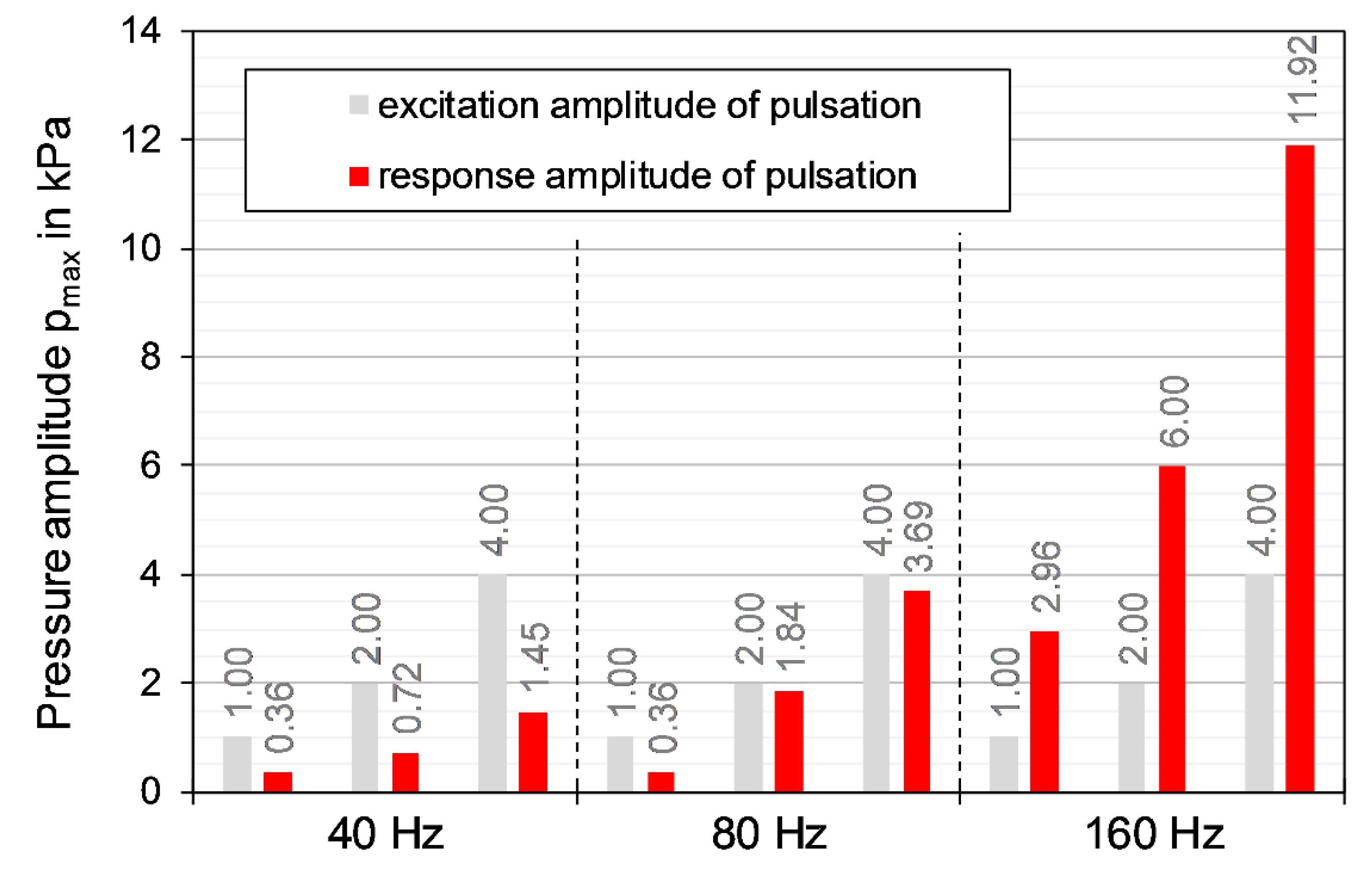One distinctive feature of Glatt’s APPtec^® method is the adjustable frequency and amplitude of the pulsation independently of other crucial processing parameters like gas temperature and mean gas flow velocity, providing a wide range of operation regimes. Typical frequencies are in-between 40–160 Hz with pulsation pressure amplitudes of up to 5 kPa. Therefore, the influence of different combinations of these two parameters on particles of different properties (especially particle size) are of special interest for a deeper understanding of process behavior and resulting product properties.

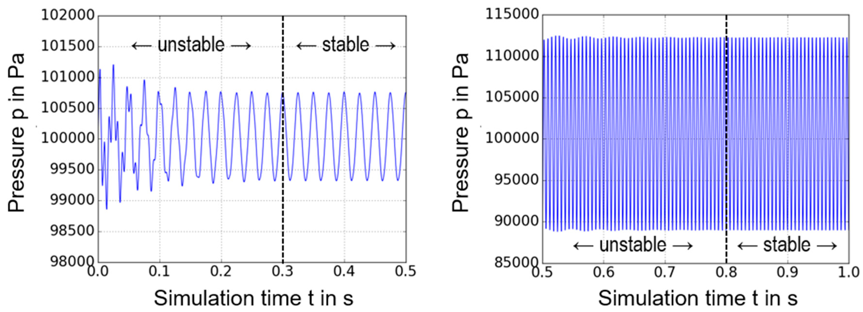
In the present work, particle formation in pulsed multiphase flow is modelled in two subsequent stages. In the first stage, gas pulsation is simulated in a vertical cylindrical pipe reactor by computational fluid dynamics method (CFD) without consideration of the solid phase. Since the solid concentration in the considered reactor with analysis of single particles is low, it is assumed that the individual particles have no influence on gas dynamics. Afterwards, obtained CFD data are revaluated and resulting flow profiles for different pulsation frequencies and amplitudes are extracted for one sinusoidal pulsation period. The extraction is started only after the stabilization of transient oscillations at the quasi-stationary point. Extracted data text files are reorganized and thereby prepared for further analysis during modeling of the solid phase. The obtained time-dependent fluid profile is then transferred to the second model, where simulation of single particle dynamics as well as heat and mass transfer is performed. A similar approach has been effectively used for the modeling of liquid injection into fluidized beds [17,18,19].

2.1. Modeling of Fluid Flow

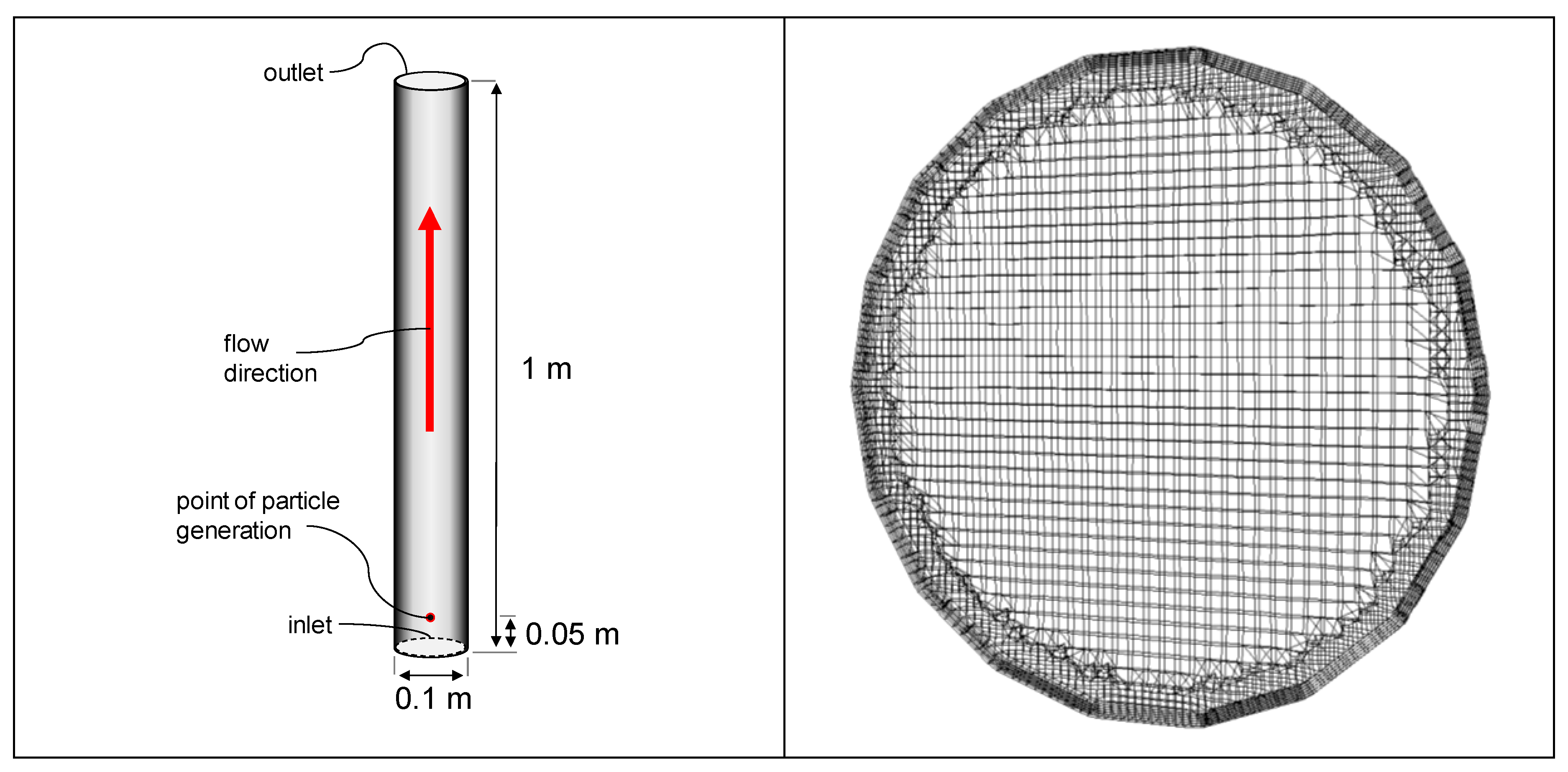
In this contribution, for CFD calculations, the open source tool OpenFOAM^® (Version 2.4.X, TheOpenFOAMFoundation Ltd., London, UK, 2011 – 2020) was used [20]. The geometry of the vertical cylindrical process chamber (d_cyl = 0.1 m, H_cyl = 1 m, see Figure 2) was drawn in CAD software SolidWorks^® and the simulation mesh was generated with hexahedral cut-cell-based OpenFOAM^® meshing tool snappyHexMesh. Meshing was performed with addition of 5 layers for higher resolution in the wall region of the cylindrical volume and a cell refinement level of 3. For the underlying block mesh, a mesh independency test was carried out. Four different refinement levels were simulated. Block mesh cell sizes $\Delta x$ of 10 mm; 5 mm; 2.5 mm and 1 mm were used. For comparison of results, the velocity profiles at heights of z = 0.05 Tablem and z = 0.95 m as well as pressure profiles at these points were compared. The percentual difference of results compared to the smallest cell size $\Delta x$ of 1 mm were up to 50% for the case of 10 mm, up to 10% for the case of 5 mm and maximum 2.5% for 2.5 mm. Based on the comparison of accuracy and calculation time, a block mesh cell size $\Delta x$ of 2.5 mm (2.5…10 times particle diameter d_p) with a total of 640,000 cells was chosen. After the addition of layers and the refinement of cells, in total, the simulation mesh contained around 1,715,000 cells of mostly hexahedral type (see Figure 2).

Simulations were carried out using the built-in SprayFOAM solver for solving combustion problems of sprays, also considering acoustic phenomena. The solver is generally based on the PIMPLE algorithm, which is a combined algorithm of the Semi-Implicit method for Pressure Linked Equations (SIMPLE) and Pressure Implicit with Splitting of Operator (PISO). Simulations were performed for turbulent flows of compressible fluids using the standard k-ε-model and Reynolds-Averaged Navier-Stokes equations (RANS). Pulsation has been modelled with a time-dependent sinusoidal gas velocity defined in the vertical direction (z):

$$u_{\mathrm{z}}\left(t\right)=u_{\mathrm{z},0}-u_{\max }·\sin \left(2\pi f_{\mathrm{puls}}t+\phi \right),$$

(1)

where $u_{\mathrm{z},0}$ is the mean vertical flow velocity, $u_{\max }$ is the pulsation velocity amplitude, $\phi$ is the angular phase shift and $f_{\mathrm{puls}}$ is pulsation frequency. The inlet velocities in radial (x, y) direction were equal to zero.

In this study, several gas flow profiles were simulated. The parameters of the investigated profiles are listed in

Table 1. Parameters for Equation (1) varied in simulation case studies.

Parameter	Symbol	Value	Unit
Mean vertical gas flow velocity	uz,0	6	m/s
Angular phase shift	φ	0	-
Pulsation pressure amplitude	pmax	0 1; 1; 2 and 4	kPa
Pulsation velocity amplitude	umax	0 1; 3; 6 and 12	m/s
Pulsation frequency	fpuls	0 1; 40; 80 and 160	Hz

¹ Reflects the stationary simulation case for comparison.

. The parameters, except pulsation velocity amplitude, were chosen based on typical operating parameters of Glatts APPtec^® measured with the powder synthesis plant ProAPP500^®. These parameters define the chosen boundary conditions for the numerical investigation. Since the acoustic behavior of the overall plant ProAPP500 is not only determined by the geometry of the pyrolysis reactor pipe, but also by duct work and gas–solid separation units, like cyclones and filters, the acoustic behavior in terms of resonance differs from the simplified reactor (only) model volume investigated in this study. Resulting pulsation amplitudes from excitation based on the chosen boundary conditions are shown and further explained in Section 3.1.

The pulsation velocity amplitude is a necessary simulation parameter derived from the pulsation frequency and pressure amplitude. Based on the theory of acoustics, the velocity pulsation amplitude $u_{\max }$ is equal to the sound particle velocity $u_{\mathrm{eff}}$, which is a function of the root mean square of the pressure amplitude, the speed of sound $c_{\max }$ and the density of the gas ${\rho }_G$ at a given temperature.

$${\mathrm{u}}_{\max }={\mathrm{u}}_{\mathrm{eff}}=\frac{{\mathrm{p}}_{\max }}{\sqrt{2}·{\mathrm{c}}_{\max }\left(\mathrm{T}\right)·{\mathsf{\rho }}_{\mathrm{G}}\left(\mathrm{T}\right)},$$

(2)

The basis for the pulsation pressure amplitude are measured values at typical operation regimes of the powder synthesis plant ProAPP500^®. For the measurement, a fast, dynamic pressure measurement with online fast Fourier transformation is used to analyze main frequencies and their respective pressure amplitudes.

In total, the variation of listed parameters provides a set of 10 different fluid flow simulations: 9 simulations with pulsation and one stationary fluid flow simulation for comparison. All other inlet condition parameters kept constant in all simulations are listed in

Table 2. Constant simulation parameters.

Parameter	Symbol	Value	Unit
Gas flow velocity at outlet	uoutlet	“zero gradient”	m/s
Gas composition
Oxygen mass fraction	wO2,inlet	0.234	kg/kg
Nitrogen mass fraction	wN2,inlet	0.766	kg/kg
Thermodynamic gas properties
Gas temperature at inlet	Tinlet	800	K
Gas temperature at outlet	Toutlet	“zero gradient”	K
Gas pressure at inlet	pinlet	“zero gradient”	kPa
Gas pressure at outlet	poutlet	100	kPa

. In order to not overdetermine the simulation system, thermodynamic gas properties are only defined either for the inlet or the outlet of the model volume. Temperature (T_outlet), velocity (u_outlet) at outlet and pressure (p_inlet) at inlet are defined as “zero gradient” and directly calculated from the given boundary conditions during simulation. Pressure at the outlet is set to ambient conditions to simulate an open pipe to the environment. Time-dependent pressure pulsation in the cylindrical volume results from the defined sinusoidal velocity excitation at the inlet. A no-slip condition is assumed for all fluid–solid boundaries, so that the gas phase will have zero velocity relative to the wall boundary. Simulation time steps and saving intervals are dependent on the actual simulated pulsation frequency and amplitude. The simulation time steps are set to be adjustable by the solver and calculated on the basis of a maximum Courant-Number Co = 0.75 [21].

$$\mathrm{Co}=\mathrm{u}·\frac{\Delta \mathrm{x}}{\Delta \mathrm{t}}=0.75,$$

(3)

where $\Delta t$ is the simulation time step, $\Delta x$ is the cell size and $u$ is the flow velocity.

The saving interval of obtained data is chosen to be 1/10 of the duration of a single pulsation period which is dependent on the simulated pulsation frequency. The sampling frequency $f_{\mathrm{samp}}$ is therefore 10 times the pulsation frequency $f_{\mathrm{puls}}$.

$${\mathrm{f}}_{\mathrm{samp}}=10·{\mathrm{f}}_{\mathrm{puls}}.$$

(4)

2.2. Modeling of Solid Phase

For the modeling of particle dynamics in the reactor, a separate sub-model was developed and implemented in C++ programming language. Here, the single particles are generated in the injection zone and afterwards each particle is treated as a separate discrete entity. It is supposed that in a steady-state regime, the gas profile is the same for different pulsation periods. Therefore, the fluid profile extracted from CFD calculations for one pulsation period is recursively repeated for a longer time interval. The fluid flow profile for one pulsation period is represented by 10 equidistant time points. Each time point is exported from the CFD calculations as an individual text file. To extract information about flow profile at any arbitrary time, linear interpolation was used. To be able to evaluate the single particle dynamics at any time and any condition of injection 40,000 particles per second are considered and simulated simultaneously.

Three main groups of time-dependent particle characteristics are studied in this contribution:

• single particle dynamics: trajectory, velocity and acceleration;
• thermal evolution: temperature, heat and enthalpy flux;
• species evolution: concentration, mass flux and size change.

To simulate time-dependent change of particle properties, the whole simulation time was discretized into smaller simulation time steps of constant size, and calculations were performed iteratively. All temperature-dependent thermodynamic properties of the fluids, such as, e.g., evaporation enthalpy, dynamic viscosity or heat conductivity, are calculated according to [22] and will not be explained in further detail.

2.2.1. Particle Dynamics

Particle dynamics were modeled with certain simplifications and assumptions. It is assumed that all particles are spherical and have the same initial size and composition. Particle–particle interaction, particle breakage or agglomeration, as well as an influence of the solid phase on gas flow are neglected. For the modeling of particle–wall interactions, it is assumed that if a particle collides with any part of the geometry, it sticks to its surface and no rebound occurs. Furthermore, a homogeneous temperature profile inside of each particle is assumed. Thus, heat conduction inside of the particles is not considered. Particle shrinking caused by the evaporation of solvent is assumed to be dependent only on the loss of volume of the solvent.

Relative velocities u_rel between particles and surrounding fluid are calculated for any time point t and particle i as the difference between gas and particle velocity u and v in all three coordinates x, y and z. To obtain gas properties such as flow velocity or temperature, the closest node to the position of the particle in the 3D simulation volume is selected

$${\mathrm{u}}_{\mathrm{rel},\mathrm{i}}\left(\mathrm{t}\right)={\mathrm{u}}_{\mathrm{i}}\left(\mathrm{t}\right)-{\mathrm{v}}_{\mathrm{i}}\left(\mathrm{t}\right).$$

(5)

The particle Reynolds number Re_p is derived by Equation (6), where ρ_f is the density of the fluid, η_f is the dynamic viscosity of the fluid and r_p is the time-dependent particle radius. The dynamic viscosity and density of the surrounding gas are calculated for each particle and time point separately. Depending on the particle’s position, the temperature of the gas of the closest node is used for the calculation of temperature-dependent gas properties as described in Section 2.2.2.

$${\mathrm{Re}}_{\mathrm{p},\mathrm{i}}\left(\mathrm{t}\right)=\frac{{\mathsf{\rho }}_{\mathrm{f},\mathrm{i}}\left(\mathrm{t}\right)·{\mathrm{u}}_{\mathrm{rel},\mathrm{i}}\left(\mathrm{t}\right)·2·{\mathrm{r}}_{\mathrm{p},\mathrm{i}}\left(\mathrm{t}\right)}{{\mathsf{\eta }}_{\mathrm{f},\mathrm{i}}\left(\mathrm{t}\right)}.$$

(6)

The drag coefficient C_D is dependent on the particle Reynolds number Re_p. For spherical particles and Re_p < 10⁵ the drag coefficient is calculated with the correlation of [23] described by:

$${\mathrm{C}}_{\mathrm{D},\mathrm{i}}\left(\mathrm{t}\right)=\frac{24}{{\mathrm{Re}}_{\mathrm{p},\mathrm{i}}\left(\mathrm{t}\right)}+\frac{4}{{\mathrm{Re}}_{\mathrm{p},\mathrm{i}}{\left(\mathrm{t}\right)}^{0,5}}+0.4.$$

(7)

The change in the velocity of the individual particle is estimated through its momentum balance. The net forces acting on the particle constitute the downward gravity force, the upward drag force and buoyancy. In this contribution the buoyancy force is neglected and resulting forces F are described by:

$${\mathrm{F}}_{\mathrm{i}}\left(\mathrm{t}\right)=0.5·{\mathsf{\rho }}_{\mathrm{f},\mathrm{i}}\left(\mathrm{t}\right)·{\mathrm{C}}_{\mathrm{D},\mathrm{i}}\left(\mathrm{t}\right)·\mathsf{\pi }·{\mathrm{r}}_{\mathrm{p},\mathrm{i}}{\left(\mathrm{t}\right)}^2·{\mathrm{u}}_{\mathrm{rel},\mathrm{i}}{\left(\mathrm{t}\right)}^2+{\mathrm{F}}_{\mathrm{g},\mathrm{i}}\left(\mathrm{t}\right).$$

(8)

Note, that due to the evaporation, the mass of particles is not constant. Detailed explanations regarding mass loss are given in the following sections related to heat and mass transfer.

To calculate changes of particle velocities v_i and coordinates $X_{\mathrm{p},\mathrm{i}}$ for each following time step $\mathrm{t}+\Delta \mathrm{t}$ the Euler integration scheme is used:

$${\mathrm{v}}_{\mathrm{i}}\left(\mathrm{t}+\Delta \mathrm{t}\right)={\mathrm{v}}_{\mathrm{i}}\left(\mathrm{t}\right)+\frac{\Delta \mathrm{t}·{\mathrm{F}}_{\mathrm{i}}\left(\mathrm{t}\right)}{{\mathrm{m}}_{\mathrm{p},\mathrm{i}}\left(\mathrm{t}\right)},$$

(9)

$$X_{\mathrm{p},\mathrm{i}}\left(\mathrm{t}+\Delta \mathrm{t}\right)=X_{\mathrm{p},\mathrm{i}}\left(t\right)+\Delta t·v_{\mathrm{i}}\left(t\right).$$

(10)

2.2.2. Heat Transfer

Thermal evolution of the particles depends on heat transfer from the surrounding gas to the particle and on solvent evaporation. The empirical Ranz and Marshall correlation defines the heat transfer between a spherical particle and the surrounding gas for a wide range of thermodynamic properties [24,25]. The calculation of the individual particle Nusselt number Nu thereby is given as:

$$N{u}_{\mathrm{p},\mathrm{i}}\left(t\right)=2+0.6·R{e}_{\mathrm{p},\mathrm{i}}{\left(t\right)}^{\frac{1}{2}}·P{r}_{\mathrm{i}}{\left(t\right)}^{\frac{1}{3}},$$

(11)

with the Prandtl number Pr, where c_P,f,i is the specific heat capacity of the fluid at constant pressure and λ_f,i is the heat conductivity of the fluid and. Fluid parameters like λ_f,i or the dynamic viscosity η_f,i are directly derived from fluid flow simulation results at the closest node to the particle i. Temperature- and pressure-dependent parameters are then calculated with polynomial functions from VDI-Wärmeatlas [22]:

$${\mathrm{Pr}}_{\mathrm{i}}\left(\mathrm{t}\right)=\frac{{\mathsf{\eta }}_{\mathrm{f},\mathrm{i}}\left(\mathrm{t}\right)·{\mathrm{c}}_{\mathrm{P},\mathrm{f},\mathrm{i}}\left(\mathrm{t}\right)}{{\mathsf{\lambda }}_{\mathrm{f},\mathrm{i}}\left(\mathrm{t}\right)}.$$

(12)

The individual gas–particle heat transfer coefficient h is derived from the Nusselt number obtained by Equation (11).

$${\mathrm{h}}_{\mathrm{i}}\left(\mathrm{t}\right)=\frac{{\mathrm{Nu}}_{\mathrm{p},\mathrm{i}}\left(\mathrm{t}\right)·{\mathsf{\lambda }}_{\mathrm{f},\mathrm{i}}\left(\mathrm{t}\right)}{{\mathrm{r}}_{\mathrm{p},\mathrm{i}}{\left(\mathrm{t}\right)}^2}.$$

(13)

The resulting heat flow $\dot{\mathrm{Q}}$ to the individual particle is described by Equation (14):

$${\dot{\mathrm{Q}}}_{\mathrm{i}}\left(\mathrm{t}\right)={\mathrm{h}}_{\mathrm{i}}\left(\mathrm{t}\right)·4\mathsf{\pi }·{\mathrm{r}}_{\mathrm{p},\mathrm{i}}{\left(\mathrm{t}\right)}^2·\left({\mathrm{T}}_{\mathrm{f},\mathrm{i}}\left(\mathrm{t}\right)-{\mathrm{T}}_{\mathrm{p},\mathrm{i}}\left(\mathrm{t}\right)\right),$$

(14)

where T_f,i and T_p,i are the time-dependent temperature of fluid and individual particle. The changes in particle temperature for each time step are calculated with respect to mass transfer and evaporation enthalpy of the liquid according to Equation (26) of Section 2.2.3.

2.2.3. Mass Transfer

Species evolution of the particles is based upon mass transfer from the particle to the surrounding gases and vice versa. In analogy to heat transfer, the empirical Ranz and Marshall correlation can be used for mass transfer calculations between a spherical particle and the surrounding gas [24]. The calculation of the individual particle Sherwood number Sh_p,i thereby is given as:

$${\mathrm{Sh}}_{\mathrm{p},\mathrm{i}}\left(\mathrm{t}\right)=2+0.6·{\mathrm{Re}}_{\mathrm{p},\mathrm{i}}{\left(\mathrm{t}\right)}^{\frac{1}{2}}·{\mathrm{Sc}}_{\mathrm{i}}{\left(\mathrm{t}\right)}^{\frac{1}{3}}.$$

(15)

The Prandtl number Pr in Equation (12) is replaced with the Schmidt number Sc,

$${\mathrm{Sc}}_{\mathrm{i}}\left(\mathrm{t}\right)=\frac{{\mathsf{\eta }}_{\mathrm{f},\mathrm{i}}\left(\mathrm{t}\right)}{{\mathsf{\rho }}_{\mathrm{f},\mathrm{i}}\left(\mathrm{t}\right)·{\mathrm{D}}_{12,\mathrm{i}}\left(\mathrm{t}\right)}.$$

(16)

For gases at low pressures, binary mass diffusivity D_12,i needed for the calculation of Sc_i is estimated according to [26] with the following conditional equation:

$${\mathrm{D}}_{12,\mathrm{i}}\left(\mathrm{t}\right)=\frac{1.43·{10}^{-3}·{\mathrm{T}}_{\mathrm{f},\mathrm{i}}{\left(\mathrm{t}\right)}^{1.75}·{\left(\frac{1}{{\mathrm{M}}_1}+\frac{1}{{\mathrm{M}}_2}\right)}^{\frac{1}{2}}}{\sqrt{2}·{\mathrm{p}}_{\mathrm{f},\mathrm{i}}\left(\mathrm{t}\right)·{\left[{\left(\sum {\Delta }_{\mathsf{\nu }1}\right)}^{\frac{1}{3}}+{\left(\sum {\Delta }_{\mathsf{\nu }2}\right)}^{\frac{1}{3}}\right]}^2},$$

(17)

where M₁, M₂ are the molar weights of substance 1 (solute) and 2 (solvent) accordingly; p_f,i is the pressure of the fluid surrounding the particle; ∑Δ_ν1, ∑Δ_ν2 are diffusion volumes of substance 1 and 2 based on functional group contributions.

The individual gas–particle mass transfer coefficient k_i is derived from the Sherwood number obtained by Equation (15)

$${\mathrm{k}}_{\mathrm{i}}\left(\mathrm{t}\right)=\frac{{\mathrm{Sh}}_{\mathrm{p},\mathrm{i}}\left(\mathrm{t}\right)·{\mathrm{D}}_{12,\mathrm{i}}\left(\mathrm{t}\right)}{2·{\mathrm{r}}_{\mathrm{p},\mathrm{i}}\left(\mathrm{t}\right)}.$$

(18)

The resulting mass flow ${\dot{\mathrm{m}}}_{\mathrm{vap},\mathrm{i}}$ of vapor from the individual particle is described by Equation (19):

$${\dot{\mathrm{m}}}_{\mathrm{vap},\mathrm{i}}\left(\mathrm{t}\right)={\mathsf{\rho }}_{\mathrm{f},\mathrm{i}}\left(\mathrm{t}\right)·{\mathrm{k}}_{\mathrm{i}}\left(\mathrm{t}\right)·4\mathsf{\pi }\Delta {\mathrm{r}}_{\mathrm{p},\mathrm{i}}{\left(\mathrm{t}\right)}^2·\left({\mathrm{Y}}_{\mathrm{P},\mathrm{sat},\mathrm{i}}\left(\mathrm{t}\right)-{\mathrm{Y}}_{\mathrm{f},\mathrm{i}}\left(\mathrm{t}\right)\right),$$

(19)

where Y_P,sat,i and Y_f,i are the time-dependent saturation humidity at the surface of each individual particle and of bulk fluid

$${\mathrm{Y}}_{\mathrm{P},\mathrm{sat},\mathrm{i}}\left(\mathrm{t}\right)=\frac{{\mathrm{M}}_1}{{\mathrm{M}}_2}·\frac{{\mathrm{p}}_{\mathrm{vap},\mathrm{i}}\left(\mathrm{t}\right)}{{\mathrm{p}}_{\mathrm{f},\mathrm{i}}\left(\mathrm{t}\right)-{\mathrm{p}}_{\mathrm{vap},\mathrm{i}}\left(\mathrm{t}\right)}.$$

(20)

Here p_vap,I is the vapor pressure for the evaporating substance at current temperature T_p,i of each individual particle, calculated with Antoine’s equation (Antoine coefficients C_A, C_B and C_C are listed in

Table 3. Initial particle and material properties.

Parameter	Symbol	Value	Unit
initial particle properties
radius	rp,0	125; 250 and 500	µm
solid weight fraction	wp,S,0	0.4	kg/kg
temperature	Tp,0	300	K
material properties of solid, liquid and gas
solid density	ρS	2000	kg/m3
liquid density	ρL	1000	kg/m3
solid heat capacity	cP,S	2500	J/kg/K
liquid heat capacity	cP,L	4200	J/kg/K
molecular weight of water	MWater	18.020	g/mol
molecular weight of pseudocomp. Air	MAir	28.949	g/mol
diffusion volume of water	∑ΔνWater	13.1	-
diffusion volume of pseudocomp. Air	∑ΔνAir	19.7	-
Antoine coefficients for Pa and K
1st; 2nd; 3rd Antoine coefficients	CA; CB; CC	23.195; −3813.98; −46.29	-

):

$$\ln {\mathrm{p}}_{\mathrm{vap},\mathrm{i}}\left(\mathrm{t}\right)={\mathrm{C}}_{\mathrm{A}}+\frac{{\mathrm{C}}_{\mathrm{B}}}{{\mathrm{C}}_{\mathrm{C}}+{\mathrm{T}}_{\mathrm{p},\mathrm{i}}\left(\mathrm{t}\right)}.$$

(21)

The solids weight fraction w_p,S,i of the individual particles changes with time by the evaporation of the solvent and is described by:

$${\mathrm{w}}_{\mathrm{p},\mathrm{S},\mathrm{i}}\left(\mathrm{t}+\Delta \mathrm{t}\right)={\mathrm{w}}_{\mathrm{p},\mathrm{S},\mathrm{i}}\left(\mathrm{t}\right)+\frac{{\mathrm{w}}_{\mathrm{p},\mathrm{S},\mathrm{i}}\left(\mathrm{t}\right)·{\dot{\mathrm{m}}}_{\mathrm{vap},\mathrm{i}}\left(\mathrm{t}\right)}{{\mathrm{m}}_{\mathrm{p},\mathrm{i}}\left(\mathrm{t}\right)}·\Delta \mathrm{t}.$$

(22)

The evaporation of the solvent causes each individual particle to shrink and to change its mass. This transient behavior is described by Equations (23) and (24), where ρ_L is the density of the evaporated liquid:

$${\mathrm{r}}_{\mathrm{p},\mathrm{i}}\left(\mathrm{t}+\Delta \mathrm{t}\right)={\mathrm{r}}_{\mathrm{p},\mathrm{i}}\left(\mathrm{t}\right)-\frac{{\dot{\mathrm{m}}}_{\mathrm{vap},\mathrm{i}}\left(\mathrm{t}\right)}{{\mathsf{\rho }}_{\mathrm{L}}·4\mathsf{\pi }·{\mathrm{r}}_{\mathrm{p},\mathrm{i}}{\left(\mathrm{t}\right)}^2}·\Delta \mathrm{t},$$

(23)

$$m_{\mathrm{p},\mathrm{i}}\left(\mathrm{t}+\Delta \mathrm{t}\right)=m_{\mathrm{p},\mathrm{i}}\left(t\right)-{\dot{m}}_{\mathrm{vap},\mathrm{i}}\left(t\right)·\Delta t.$$

(24)

On the basis of the evaporated mass of liquid ${\dot{\mathrm{m}}}_{\mathrm{vap},\mathrm{i}}$ the resulting enthalpy stream ${\dot{\mathrm{H}}}_{\mathrm{vap},\mathrm{i}}$ from the gas to the liquid and vapor at the surface of each individual particle is calculated according to Equation (25), where Δh_vap,i(T_f,i) is the temperature-dependent evaporation enthalpy of the liquid and c_P,vap,i is the specific heat capacity of the vapor at constant pressure:

$${\dot{\mathrm{H}}}_{\mathrm{vap},\mathrm{i}}\left(\mathrm{t}\right)={\dot{\mathrm{m}}}_{\mathrm{vap},\mathrm{i}}\left(\mathrm{t}\right)·\left(\Delta {\mathrm{h}}_{\mathrm{vap},\mathrm{i}}\left({\mathrm{T}}_{\mathrm{f},\mathrm{i}}\right)+{\mathrm{c}}_{\mathrm{P},\mathrm{vap},\mathrm{i}}·{\mathrm{T}}_{\mathrm{f},\mathrm{i}}\left(\mathrm{t}\right)\right).$$

(25)

The individual particle temperature T_p,i is calculated as:

$${\mathrm{T}}_{\mathrm{p},\mathrm{i}}\left(\mathrm{t}+\Delta \mathrm{t}\right)={\mathrm{T}}_{\mathrm{p},\mathrm{i}}\left(\mathrm{t}\right)+\frac{{\dot{\mathrm{Q}}}_{\mathrm{i}}\left(\mathrm{t}\right)-{\dot{\mathrm{H}}}_{\mathrm{vap},\mathrm{i}}\left(\mathrm{t}\right)}{{\mathrm{m}}_{\mathrm{p},\mathrm{i}}\left(\mathrm{t}+\Delta \mathrm{t}\right)·{\mathrm{c}}_{\mathrm{P},\mathrm{S},\mathrm{i}}}·\Delta \mathrm{t}.$$

(26)

2.2.4. Calculation Algorithm

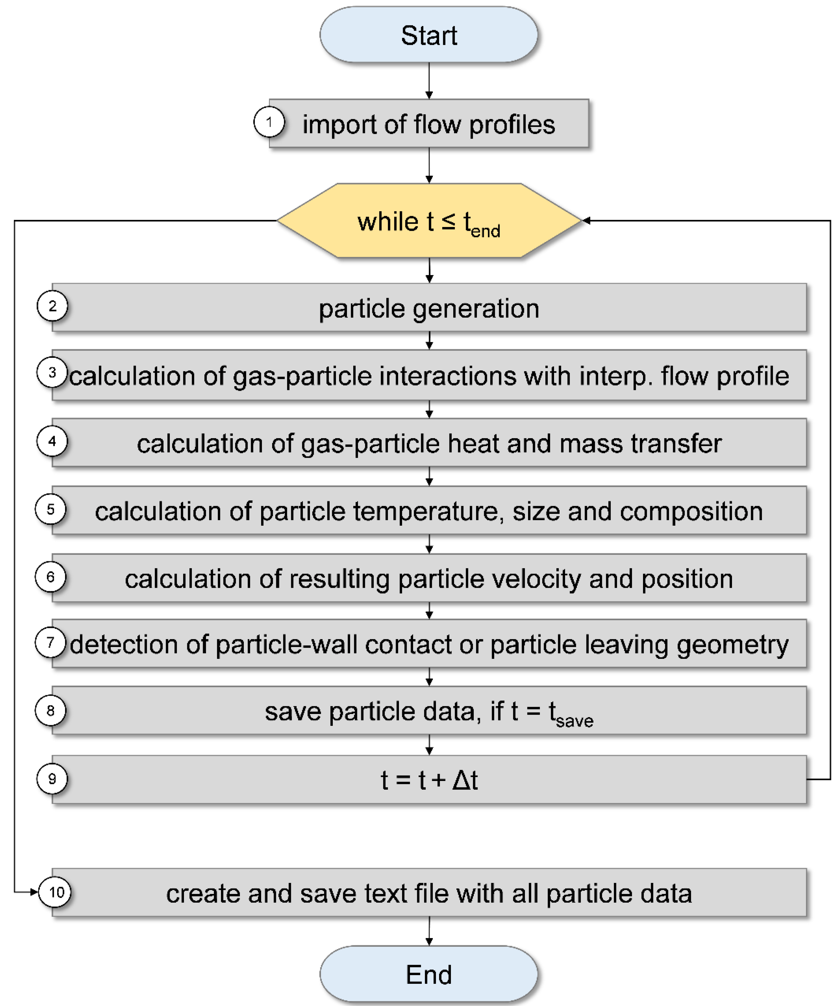
The overall calculation algorithm for the particle modeling as discrete elements unilaterally coupled with CFD gas flow profiles is shown in Figure 3. At start of the simulation, flow profiles for all 10 time points are imported. This data is stored in RAM to increase the performance of data access. Afterwards, calculations are performed iteratively with a simulation time step Δt until the end simulation time t_end.

In each simulation time step $\Delta t·{\dot{N}}_{\mathrm{p}}$ new particles (droplets) are generated, where ${\dot{N}}_{\mathrm{p}}$ is the particle generation rate. Particles are generated in a point-like source (x = 0; y = 0 and z = 0.05) with an initial velocity in radial and vertical direction. The distribution of initial particle velocity is defined with a normal distribution. The parameters of the distribution are listed in

Table 4. Simulator settings.

Parameter	Symbol	Value	Unit
time variables
simulation time step	Δt	1.25 × 10−4	s
end time	tend	1	s
saving interval	tsave	6.25 × 10−3	s
particle generation variables
generation rate	${\dot{N}}_{\mathrm{p}}$	40.000	1/s
generation origin	x; y; z	0; 0; 0.05	m
initial velocity mean/deviation	vx(0); vy(0); vz(0)	0/0.1; 0/0.1; 0.5/0.2	m/s

. These parameters were chosen to cover all possible injection angles in a full cone with an opening angle of 30°, which is a typical spray cone geometry for this type of application. In the following algorithm stage, the forces acting on particles from the fluid are calculated. To obtain flow properties at a specific time point, linear interpolation of existing CFD data is performed. Gas particle interactions and resulting particle motion with respect to velocities, trajectories and positions are then calculated. On the basis of the resulting gas–particle heat and mass transfer new particle properties, such as temperature, solids weight fraction and particle size, are obtained. As a next step wall contacts or particles leaving the volume through the top are detected and correspondent elements are deactivated. Obtained information is saved into RAM with saving step t_save. The algorithm is repeated until the defined end time t_end is reached. In the end, all data are saved to a text file. The format of saved text files is optimized for further analysis in the component-based framework MUSEN [27].

2.2.5. Parameters for Particle Simulation

In this study, particles are composed of a model solid material and water as the solvent liquid. Besides a variation of particle size, all other parameters are kept constant for all simulation case studies. Table 3 lists all initial particle and material properties. Simulation time steps and saving intervals as well as the end time are kept constant for all simulation cases. To keep the computational effort and required storage space comparably low in all studies, one second of process time was simulated. The analysis of simulation results for longer time intervals such as 2 or 5 seconds shows that already after 1 second, a convergent solution is reached. The origin for particle generation was chosen to be in the center and slightly above the inlet cross section of the cylinder. The particle inlet velocity is set to be slow compared to the surrounding gas velocities. All simulation parameters and other boundary conditions are kept constant as well (see Table 4).

3. Results

The basis for particle simulation is obtained by CFD flow simulations. Therefore, the CFD simulation results will be outlined before the discussion of the resulting particle dynamics occurs.

3.1. Fluid Flow Profile

The variation of pulsation parameters results in different flow profiles obtained by CFD simulations. The sinusoidal velocity excitation at the inlet of the simulated volume leads to a transient oscillation that becomes stabilized after a certain simulation time. The duration of this start-up phase depends on the amplitude, frequency and acoustic response of the system. As shown in Figure 4, the time for stabilization is longer if the excitation is stronger, meaning higher amplitudes and frequencies.

If the frequency of the excitation at the inlet is in resonance with the simulated volume, the response amplitudes of the pressure pulsation exceed the amplitudes of excitation (see 160 Hz in Figure 5). On the other hand, very low frequencies (in this case 40 Hz) that are not in resonance with the simulated volume lead to a heavy damping of the resulting pressure amplitudes. At 80 Hz, the response amplitude of the pressure pulsation is slightly damped and nearly of the same order as the amplitude of excitation. An exception can be observed for the lowest excitation amplitude at 80 Hz. The response amplitude is heavily damped and is similar to the one of 40 Hz.

Figure 6 shows different vertical flow velocity profiles over the cross section of the simulated volume. Compared to the stationary flow profile without pulsation (û = 0 m/s), the minimum and maximum vertical flow velocity profiles for one pulsation period are significantly changed. With increasing pulsation amplitude, the overall changes in velocity are intensified and—especially in the region close to the wall of the volume—the back flow is increased, with a bigger radial influence on the velocity profile.

3.2. Behaviour of Solid Phase

Based on the CFD simulations, particle simulations were carried out with parameter variations listed in Section 2.1. The simulations are evaluated with respect to particle dynamics, influencing the particle residence time t_R in the simulated volume and particle yield at the outlet of the volume, as well as with respect to gas–particle heat and mass transfer.

3.2.1. Particle Dynamics

The resulting particle dynamics for different flow conditions are shown in Figure 7 (low amplitude 3 m/s), Figure 8 (medium amplitude 6 m/s) and Figure 9 (high amplitude 12 m/s) for a simulation time point of t_sim = 0.975 s. The visualization of the simulation results was carried out with the component-based framework MUSEN [27].

Three different particle sizes (125 µm (a), 250 µm (b) and 500 µm(c)) are shown in each figure. Each particle size is displayed for every four frequencies (0; 40; 80 and 160 Hz). For better visibility during post-processing, all particle sizes were scaled to the biggest particle size with a radius of 500 µm. It can be observed that different particle grouping effects occur independent of particle size, pulsation amplitude and frequency. In general, the number of generated particle groups over the height of the simulated volume is increased by an increase of the pulsation frequency and particle size and a decrease of the pulsation amplitude.

At certain parameter combinations, e.g., for a frequency of 80 or 160 Hz in Figure 8c, the particle grouping cannot be visually identified. In these cases, the number of generated groups is high enough to blur the individual groups into a fully developed cone as seen in all stationary cases (0 Hz), where definitely no particle groups can be present. Particle grouping can be traced back to continuous particle injection with a given initial injection speed in a non-stationary flow field. Particles injected during the acceleration phase (positive velocity amplitude in z-direction of one oscillation period) will have a higher transport velocity at the time of injection than particles injected during the deceleration phase (negative velocity amplitude in z-direction of the same oscillation period). This effect in the starting phase of the transport is directly influenced by the amplitude and frequency, which can be seen as the intensity and duration of deflection, and the particle size, which defines the mass inertia. This explains why groups of big particles are closer to each other than groups of small particles at otherwise same conditions.

Groups of the same particle size are further away from each other at higher amplitudes and closer together for increased frequencies at otherwise constant conditions.

Furthermore, in comparison with the stationary flow, it can be seen that the geometry of the particle spout is constricted with pulsation velocity amplitudes higher than the mean flow velocity (Figure 8 and Figure 9) and widened with pulsation velocity amplitudes lower than the mean flow velocity of the gas (Figure 7). This effect is further influenced by the consideration of larger particle sizes. In the case of Figure 7, on the right (c), it is clearly visible that particles with a radius of 500 µm are not properly transported out of the simulated volume. The widening and constriction as well as an insufficient pneumatic transport of the particles has an effect on the particle yield.

3.2.2. Particle Yield

Particle yield is defined as the fraction of particles having left the simulated volume over the defined outlet. Moreover, the fraction of individual particles that have experienced a wall contact is analyzed. It is assumed that all particles that are not completely dried and become in contact with the wall of the geometry will stick to it as a worst-case scenario. Their last data of activity is saved. From that point on, they will not be considered for further simulation time steps.

Figure 10 shows the results for particle yield or loss considerations as the fraction of particles having left the volume through its outlet (yield) and the fraction of particles having experienced a wall contact (loss). It can be seen that the particle yield is influenced with the variation of the pulsation parameters. Compared to stationary flow, the particle yield is enhanced for all frequencies at medium (6 m/s) and high (12 m/s) pulsation velocity amplitudes. For the medium amplitude, the yield for the biggest particle size with a radius of 500 µm is roughly 0.83 for all frequencies, whereas the yield for the lowest particle size with a particle radius of 125 µm is 0.98 and higher for all frequencies. Compared to an amplitude of 6 m/s, an amplitude of 12 m/s results in a yield of 0.98 and above for all particle sizes. For low (3 m/s) pulsation velocity amplitudes an enhancement can only be observed for the smallest particle size. For the biggest particle size almost all particles experience a wall contact leading to a particle yield going close to zero. This can be linked to the findings in the section of particle dynamics. For these cases, a widening of the spout can be observed, which enhances the chances of a wall collision and, furthermore, the insufficient pneumatic transport of particles occurs.

3.2.3. Mean Particle Residence Time and Gas–Particle Heat and Mass Transfer

Particle properties, such as particle temperature T_p and particle solids mass fraction w_p,S at the outlet of the simulation domain are influenced by predominating heat and mass transfer in combination with the mean residence time t_R resulting from different pulsation parameters. Figure 11 shows the normalized mean heat transfer coefficient h_norm for two different pulsation frequencies in relation to initial particle radius and pulsation flow velocity amplitude. Mean heat transfer coefficients are normalized to the values of stationary gas flow, which also gives information about the heat transfer enhancement factor. An increase of the pulsation velocity amplitude enhances the heat transfer compared to stationary gas flow, except for the cases that have insufficient pneumatic transport. Comparing the minimum and maximum frequency shows a negligible influence on the mean heat transfer enhancement. The maximum enhancement factor for 40 Hz is 1.395 compared to 1.386 for 160 Hz at otherwise same conditions. Neglecting the insufficient pneumatic transport of bigger particles for the discussed cases, the overall range of heat transfer enhancement is in-between 1.063 and 1.395, where a higher enhancement can be observed for smaller particles. Because of the analogy between heat and mass transfer, mass transfer results will not be further discussed at this point.

Table 5. Mean particle properties and residence times at the outlet of the simulated volume independent of initial particle size and gas pulsation parameters.

fpuls	umax	rp (t = 0)
		125 µm			250 µm			500 µm
		tR in ms	Tp in K	wp,S in g/kg	tR in ms	Tp in K	wp,S in g/kg	tR in ms	Tp in K	wp,S in g/kg
0 Hz	0 m/s	213	341.2	894	280	341.4	522	398	341.4	440
40 Hz	3 m/s	175	341.6	837	410	341.4	591	946	341.5	513
	6 m/s	100	341.6	616	179	341.5	473	269	340.1	420
	12 m/s	55	341.7	513	90	341.3	434	126	333.3	407
80 Hz	3 m/s	175	341.6	837	410	341.4	592	943	341.5	513
	6 m/s	101	341.6	616	179	341.5	473	269	340.1	420
	12 m/s	56	341.8	514	90	341.3	434	126	333.3	407
160 Hz	3 m/s	175	341.6	838	410	341.4	592	946	341.5	513
	6 m/s	101	341.6	616	179	341.4	473	269	340.1	420
	12 m/s	56	341.7	515	90	341.2	434	126	333.3	407

shows the correlation between resulting residence times and mean particle temperatures as well as mean particle solids mass fraction independent of varied pulsation parameters and particle size. Taking a closer look at the mean residence times for different particle sizes, a reduction of the mean residence time can be observed with an increase of the pulsation amplitude compared to the stationary gas flow. In equal measure, pulsation frequency has a negligible influence on the same. As discussed in Section 3.2.1, the insufficient pneumatic transport of coarser particles (250 µm and 500 µm) can also be observed in terms of prolonged mean residence times for the lowest pulsation velocity amplitude. In terms of temperature T_p, a clear differentiation can be observed for the largest particles at the highest velocity pulsation amplitude. All other mean particle temperatures at the outlet of the simulated cylindrical volume are in the range of 340.1 – 341.8 K, whereas the mean outlet temperature of the other cases’ particles is as low as approximately 333.3 K.

Even though the mean heat and mass transfer coefficient for these cases is higher compared to the other cases and the mean residence time is more than two-times longer than for the smallest particle, the larger particle size and associated increase of volume and mass to the power of 3 cannot be compensated. This correlation can also be seen for the solids mass fraction w_p,S of the particles. In terms of this solid mass fraction of the particles at the outlet of the simulated volume, a bigger influence can be observed. By neglecting simulation cases with insufficient pneumatic transport, a clear and obvious trend for the solid mass fraction can be identified. The bigger the particle and the shorter the residence time, the lower the resulting solid mass fraction at the outlet of the simulated volume will be with increased velocity pulsation amplitude.

3.2.4. Residence Time Distribution

Particle dynamics resulting from different pulsation parameters and concomitant particle residence time distributions have an influence on the homogeneity of particle properties at the outlet of the simulated cylindrical volume. Figure 12, Figure 13 and Figure 14 show resulting particle residence time distributions as number-density distributions q₀ for different initial particle sizes independent of pulsation parameters.

The width of each residence time class is chosen to be 1 millisecond. Figure 12 shows the resulting residence time distributions for an initial particle radius r_p,0 of 125 µm. Particle residence times for stationary flow (a) are characterized by a narrow monomodal distribution with a distribution width of 9 ms. A pulsation amplitude of 3 m/s (b) also shows monomodal residence time distributions for pulsation frequencies of 80 and 160 Hz but compared to (a) with wider distribution widths of 22 and 24 ms. At a pulsation frequency of 40 Hz, the residence time distribution is the widest with a distribution width of 30 ms and does not show a clear monomodal shape. Compared with a pulsation amplitude of 6 m/s (c), a frequency of 40 Hz at u_max = 3 m/s indicates the development of bimodal distributions under pulsating conditions. At a pulsation amplitude of 6 m/s, bimodal residence time distributions are generated by pulsation frequencies of 40 and 80 Hz with distribution widths of 17 and 12 ms. A pulsation frequency of 160 Hz results in a monomodal distribution with a distribution width of 10 ms. The highest velocity pulsation amplitude of 12 m/s (d) shows bimodal residence time distributions for all investigated frequencies. The resulting distribution widths are 15 ms for f_puls = 40 Hz, 9 ms for f_puls = 80 Hz and 6 ms for f_puls = 160 Hz. Compared to stationary flow (a) only pulsation parameter combinations of an amplitude of 12 m/s and pulsation frequencies of 80 and 160 Hz indicate equal or higher homogeneity for the product particles obtained at the outlet of the simulated volume due to the lower width of residence time distributions.

Figure 13 shows resulting residence time distributions for an initial particle radius of 250 µm. Similar to Figure 12, particle residence times for stationary flow (a) are characterized by a narrow monomodal distribution with a distribution width of 21 ms. Comparing (a) in Figure 13 to (a) in Figure 12, the residence time distribution for particles at the outlet of the simulated volume is wider. Insufficient pneumatic transport at a low velocity pulsation amplitude of 3 m/s for all investigated frequencies with an initial radius of 250 µm can also be detected in the residence time distributions (b). As discussed in Section 3.2.1, for these simulation cases, the mean residence time is prolonged. The distribution curves appear “spiky” and the widths are the widest between 63 and 71 ms. At a pulsation amplitude of 6 m/s (c) in Figure 13a bimodal residence time distribution is generated by a pulsation frequency of 40 Hz with a distribution width of 24 ms. Compared to the obtained bimodal residence time distribution for particles with the smallest investigated initial radius in (c) of Figure 12, a pulsation frequency of 80 Hz for medium-sized particles results in a monomodal residence time distribution with a distribution width of 21 ms. The distribution width of monomodal distributed residence times at 160 Hz is 0.019 ms. The highest pulsation amplitude u_max = 12 m/s (d) only shows bimodal residence time distributions for frequencies of 40 and 80 Hz. The resulting distribution widths are 16 ms for 40 Hz, 1 ms for 80 Hz and 7 ms for 160 Hz, whereas the narrowest distribution is of monomodal shape. Compared to stationary flow (a), only pulsation parameter combinations of an amplitude 6 m/s and pulsation frequencies 80 and 160 Hz, as well as an amplitude 12 m/s at all pulsation frequencies, indicate equal or higher homogeneity for the product particles obtained at the outlet of the simulated volume. Figure 14 shows resulting residence time distributions for the biggest investigated initial particle radius of 500 µm. Due to the insufficient pneumatic transport, for the lowest pulsation amplitude u_max = 3 m/s, particle residence time distributions could not be evaluated. Therefore, Figure 14 only shows results for the cases of stationary flow, as well as medium and maximum investigated pulsation amplitude. Compared to Figure 12 and Figure 13, particle residence times for stationary flow (a) are not characterized by a narrow monomodal distribution. The distribution width is 50 ms and is also the highest of all cases for the biggest particles. A pulsation amplitude of 6 m/s (c) shows monomodal residence time distributions for pulsation frequencies of 80 and 160 Hz and compared to stationary flow (a) with narrower distribution widths of 41 and 38 ms. At a pulsation frequency of 40 Hz, the residence time distribution does not show a clear monomodal shape. The distribution width is 48 ms and is still lower than the width for the stationary flow.

For the highest investigated pulsation amplitude of 12 m/s (d), bimodal residence time distributions are found for frequencies of f_puls = 40 and 80 Hz and a monomodal residence time distribution is found for 160 Hz. The resulting distribution widths are 20 ms for frequency 40 Hz, 14 ms for 80 Hz and 12 ms for 160 Hz. Generally, all cases with medium (c) and maximum (d) investigated pulsation amplitudes deliver higher product-particle homogeneity compared to stationary flow (a).

The generation of bimodal residence time distributions can be linked to the formation of particle groups as discussed in Section 3.2.1. Particles are continuously injected at different times of the overlying non-stationary pulsation of the gas flow. Particles injected during the acceleration phase (positive velocity amplitude in z-direction of one oscillation period) will have a shorter residence time than particles injected during the deceleration phase (negative velocity amplitude in z-direction of the same oscillation period). This leads to the formation of two main groups of particles (accelerated and decelerated at the point of injection), which can be detected in a bimodal residence time distribution. Essentially, this leads to the assumption that all pulsating cases would result in bimodal distributed residence times of particles in the simulated volume. As pointed out in Section 3.2.1, at certain parameter combinations, the number of groups blur into a continuous flow, where the individual particle groups cannot be identified anymore.

4. Discussion

In this contribution, CFD simulations combined with discrete particle simulations were used to investigate gas–particle micro-processes in pulsed gas–solid multiphase flows. On the basis of typical operating parameters of Glatt’s APPtec^® method, parameters for variation of pulsation amplitude and frequency were selected and pulsed gas flow-induced single particle dynamics as well as the resulting gas–particle heat and mass transfer was derived for three exemplary particle sizes.

In comparison to stationary gas flow, an enhancement of heat and mass transfer could be identified with the increase of the pulsation amplitude and a decrease of particle size. Enhancement factors vary between 1.1 and 1.4. Furthermore, it was found that particle yield, grouping effects and particle residence time in the simulated volume can be influenced by the adjustment of pulsation parameters. The most influencing parameter was identified to be the amplitude of the pulsation. For pulsation amplitudes lower than the mean gas flow velocity, mean particle residence times are extended compared to the stationary flow case, and additionally the yield decreases because of a higher number of wall contacts. Higher pulsation amplitudes than the mean gas flow velocity result in a shortening of particle residence times and an increase of the particle yield.

Pulsation frequency of the excitation plays a minor role, when looking at mean values of heat and mass transfer as well as particle residence time. By evaluating the distributed parameters, such as the resulting particle residence time distribution at the outlet of the simulated volume, frequency shows a bigger influence. In comparison, narrower residence time distribution graphs also result in narrower distributions of other product properties which leads to an optimized product homogeneity. Besides the overall ranges of mean particle residence times, the corresponding shapes of particle residence time distributions are mostly bimodal and dependent on the investigated initial particle size as well as on the level of excitation under pulsating conditions. For the smallest investigated particles, the residence time distribution becomes narrower with frequencies from 80 Hz and above for pulsation amplitudes higher than the mean gas flow velocity compared to the stationary case. For pulsation amplitudes lower than or equal to the mean gas flow velocity, the frequency is still influential and delivers narrower distributions with increasing frequencies. However, particle residence time distributions are wider compared to the stationary flow for these simulation cases. For medium-sized particles, in comparison to the stationary flow case, the residence time distribution becomes narrower with frequencies from 80 Hz and above for pulsation amplitudes equal to the mean gas flow velocity. For the highest pulsation amplitude, this relation is valid for all frequencies. The behavior of medium-sized particles at pulsation amplitudes lower than the mean gas flow velocity is similar to the behavior of the smallest particles. The biggest particles show a constriction of the residence time distribution for all pulsating cases with sufficient pneumatic transport. A different and independent experimental study carried out by Alexander Schmidt [28] focusses on spray pyrolysis of the material system manganese nitrate to form manganese oxide. With a variation of the same frequencies (40; 80 and 160 Hz), the influence on product homogeneity was studied for two particle sizes classes. Particle sizes were varied by two different atomization pressure settings. Homogeneity has been evaluated by the span of the particle size number distribution.

Comparing the values shown in

Table 6. Span of particle size number distribution for different particle sizes independent of pulsation frequency adapted from [28].

Frequency in Hz	Span of Number Particle Size Distribution [span = (q90,0 – q10,0)/q50,0]
	High atomization pressure (low particle sizes)	Low atomization pressure (large particle sizes)
0 “stationary”	1.523	4.219
40	3.286	4.700
80	2.730	3.875
160	1.923	3.813

, spans of particle size distributions become narrower with increased pulsation frequencies for both particle size classes, which is in accordance with the findings presented in this study. Comparing the stationary case with cases with pulsation, a similar result as in this presented study can be observed. For low particle sizes, the span of the particle-size number distribution is the lowest for the stationary case. For larger particle sizes, the span becomes smaller for frequencies from 80 Hz and above.

As a next step, representative experimental studies are carried out to validate the simulation results. On one hand, experiments consist of drying experiments, with a variation of the same parameters to identify the influences of pulsation parameters on particle-size distribution and moisture content. On the other hand, particle dynamics are analyzed with high speed camera caption and a transparent cylindrical volume of the same dimensions as used in the simulation studies to identify grouping and spout constriction behavior independent of the particle size and pulsation parameters applied.

5. Conclusions

Based on the findings of this study, qualitative parameter sensitivities can be summarized (see

Table 7. Qualitative parameter sensitivities.

Influenced Parameter	Particle Size	Pulsation Amplitude	Pulsation Frequency
Mean residence time	+	–
Mean particle temperature	(–) 1
Mean solids mass fraction	–	–
Mean heat and mass transfer	–	(+) 2
Variance of distributed parameters	+	(–) 3	(–) 3
Particle grouping	+	–	+
Spout constriction	–	+

¹ only valid for biggest particles and maximum pulsation amplitude. ² only valid for medium and maximum pulsation amplitude. ³ only valid for comparison of cases with pulsation.

). For example: An increase “+” of particle size results in an increase “+” of mean residence time at otherwise constant conditions. The increase of pulsation frequency has no or negligible “ “ influence on mean residence time. An increase of pulsation amplitude results in a restricted decrease “(-)” of the variance of distributed parameters. In this case, restricted means that the decrease is only valid while comparing simulation cases with pulsation. It is partly valid for stationary and pulsating conditions to be selected as simulation parameters, such as, e.g., biggest particles.

In conclusion, it can be outlined that by varying and applying appropriate pulsation parameters on pulsed multiphase flows for particle treatment, such as frequency and amplitude of pulsation in relation to the mean gas flow velocity, product particle properties can be tailored to the needs of the subsequent application by influencing distributed parameters or increasing the overall yield, although the mean values of the distributed parameters remain similar.

References

1. Wold, A.; Gao, Y.-M.; Miller, D.; Kershaw, R.; Dwight, K. Chapter 19, Synthesis of catalytic materials by Spray Pyrolysis. In Advanced Catalysts and Nanostructured Materials, Modern Synthetic Materials, 1st ed.; Moser, W., Ed.; Academic Press: New York, NY, USA, 1996; pp. 505–514. [Google Scholar]
2. Jung, D.S.; Ko, Y.N.; Kang, Y.C.; Park, S.B. Recent progress in electrode materials produced by spray pyrolysis for next-generation lithium ion batteries. Adv. Powder Technol. 2014, 25, 18–31. [Google Scholar] [CrossRef]
3. Patil, P.-S. Versatility of chemical spray pyrolysis technique. Mater. Chem. Phys. 1999, 59, 185–198. [Google Scholar] [CrossRef]
4. Kudra, T. Pulse-combustion drying: Status and potentials. Drying Technol. 2008, 26, 1409–1420. [Google Scholar] [CrossRef]
5. Kudra, T.; Mujumdar, A.S. Advanced Drying Technologies, 2nd ed.; CRC Press: Boca Raton, FL, USA, 2009. [Google Scholar]
6. Widiyastuti, W.; Wang, W.; Purwanto, A.; Lenggoro, I.W.; Okuyama, K. A Pulse Combustion-Spray Pyrolysis Process for the Preparation of Nano- and Submicrometer-Sized Oxide Particles. J. Am. Ceram. Soc. 2007, 90, 3779–3785. [Google Scholar] [CrossRef]
7. Glatt Ingenieurtechnik GmbH: APPtec® Brochure; Glatt Ingenieurtechnik GmbH: Weimar, Germany, 2019.
8. Jacob, M.; Teiwes, A.; Jähnert, T. Glatt Ingenieurtechnik GmbH.; DE 10 2018 205 152.6; Glatt Ingenieurtechnik GmbH: Weimar, Germany, 2018. [Google Scholar]
9. Meng, X.; Jong, W.; Kudra, T. A state-of-the-art review of pulse combustion: Principles, modeling, applications and R&D issues. Renew. Sustain. Energy Rev. 2016, 55, 73–114. [Google Scholar]
10. Carvalho, J.A., Jr. Behaviour of solid particles in pulsating flows. J. Sound Vib. 1995, 185, 581–593. [Google Scholar] [CrossRef]
11. Sazhin, S.; Shakked, T.; Sobolev, V.; Katoshevski, D. Particle grouping in oscillating flows. Eur. J. Mech. B/Fluids 2008, 27, 131–149. [Google Scholar] [CrossRef]
12. Liu, X.D.; Cao, C.W.; Lang, Z.H. Heat transfer between materials and unsteady airflow from Helmholtz type combustor. Dry. Technol. 2001, 19, 1939–1948. [Google Scholar] [CrossRef]
13. Kudra, T.; Benali, M.; Zbicinski, I. Pulse Combustion Drying: Aerodynamics, Heat Transfer, and Drying Kinetics. Dry. Technol. 2003, 21, 629–655. [Google Scholar] [CrossRef]
14. Mahapatraa, P.S.; Mukhopadhyay, A.; Panchagnula, M.V. Dispersion of Polydisperse Droplets in a Pulsating Flow Field. Procedia IUTAM 2015, 15, 242–248. [Google Scholar] [CrossRef] [Green Version]
15. Xiao, Z.; Xie, X.; Yuan, Y.; Liu, X. Influence of Atomizing Parameters on Droplet Properties in a Pulse Combustion Spray Dryer. Dry. Technol. 2008, 26, 427–432. [Google Scholar] [CrossRef]
16. Dong, L.; Zhao, Y.; Xie, W.; Duan, C.; Li, H.; Hua, C. Insights in active pulsing air separation technology for coarse coal slime by DEM-CFD approach. J. Cent. South. Univ. 2013, 20, 3660–3666. [Google Scholar] [CrossRef]
17. Dosta, M.; Antonyuk, S.; Heinrich, S. Multiscale simulation of fluidized bed granulation process. Chem. Eng. Technol. 2012, 35, 1373–1380. [Google Scholar] [CrossRef]
18. Heinrich, S.; Dosta, M.; Antonyuk, S. Multiscale analysis of a coating process in a Wurster fluidized bed apparatus. In Mesoscale Modeling in Chemical Engineering Part I.; Guy, B.M., Jinghai, L., Eds.; Advances in Chemical Engineering, Academic Press: London, UK, 2015; pp. 83–135. [Google Scholar]
19. Dosta, M. Modular based simulation of single process units. Chem. Eng. Technol. 2019, 42, 699–707. [Google Scholar] [CrossRef]
20. Weller, H.G.; Tabor, G.; Jasak, H.; Fureby, C. A tensorial approach to computational continuum mechanics using object-oriented techniques. Comput. Phys. 1998, 12, 620–631. [Google Scholar] [CrossRef]
21. Courant, R.; Friedrichs, K.; Lewy, H. Über die partiellen Differenzengleichungen der mathematischen Physik. Math. Ann. 1928, 100, 32–74. [Google Scholar] [CrossRef]
22. VDI e.V. (Hrsg.). VDI-Wärmeatlas©; Springer-Verlag: Berlin/Heidelberg, Germany, 2013. [Google Scholar]
23. Molerus, O. Principles of Flow in Disperse Systems; Chapman & Hall: Berlin, Germany, 1993. [Google Scholar]
24. Ranz, W.E.; Marshall, W.R. Evaporation from drops. Chem. Eng. Prog. 1952, 48, 141–146. [Google Scholar]
25. Aissa, A.; Abdelouahab, M.; Noureddine, A.; Elgananoui, M.; Pateyron, B. Ranz & Marshall correlation limits for a sphere and its surrounding gases at high temperature. Thermal Sci. 2015, 19, 1521–1528. [Google Scholar]
26. Fuller, E.N.; Ensley, K.; Giddings, J.C. Diffusion of halogenated hydrocarbons in helium. The effect of structure on collision cross sections. J. Phys. Chem. 1969, 73, 3679–3685. [Google Scholar] [CrossRef]
27. Dosta, M.; Antonyuk, S.; Heinrich, S. Multiscale simulation of agglomerate breakage in fluidized beds. Ind. Eng. Chem. Res. 2013, 52, 11275–11281. [Google Scholar] [CrossRef]
28. Schmidt, A. Experimentelle Prozessanalyse der Sprühkalzination von Mangandioxid im pulsierenden Heißgasstrom. Master’s Thesis, University of Applied Science–Ernst-Abbe-Hochschule Jena, Jena, Germany, 2020. [Google Scholar]
Figure 1. Overall process principle of Glatts APPtec®.
Processes 08 00815 g001
Figure 2. Left: Geometry of the vertical cylindrical process chamber. Right: Cross-sectional view of one cell plane for fluid flow simulations containing of 1,715,000 with maximum cell size of 2.5 mm.
Processes 08 00815 g002
Figure 3. Calculation algorithm for discrete particle model.
Processes 08 00815 g003
Figure 4. Stabilization time for two different simulation cases. Low excitation with stabilization after approximately 0.3 s (left) and high excitation with stabilization after approximately 0.8 s (right).
Processes 08 00815 g004
Figure 5. Response amplitudes of the pressure pulsation independent of frequency and amplitude of excitation.
Processes 08 00815 g005
Figure 6. Cross-sectional computational fluids dynamic method (CFD) vertical minimum and maximum velocity profiles for different pulsation amplitudes at a pulsation frequency of 40 Hz and stationary flow (û = 0 m/s).
Processes 08 00815 g006
Figure 7. Particle dynamics and particle grouping effects independent of particle size (125 µm (a), 250 µm (b) and 500 µm (c)) as well as frequency (for each particle size from 0 Hz (left) to 160 Hz (right)) for a velocity pulsation amplitude of umax = 3 m/s.
Processes 08 00815 g007
Figure 8. Particle dynamics and particle grouping effects independent of particle size (125 µm (a), 250 µm (b) and 500 µm (c)) as well as frequency (for each from 0 Hz (left) to 160 Hz (right)) for a velocity pulsation amplitude of umax = 6 m/s.
Processes 08 00815 g008
Figure 9. Particle dynamics and particle grouping effects independent of particle size (125 µm (a), 250 µm (b) and 500 µm (c)) as well as frequency (for each from 0 Hz (left) to 160 Hz (right)) for a velocity pulsation amplitude of umax = 12 m/s.
Processes 08 00815 g009
Figure 10. Comparison of particle yield and loss for all different simulation cases independent of initial particle size (125; 250 and 500 µm), pulsation frequency (0; 40; 80 and 160 Hz) and pulsation velocity amplitude (0; 3; 6 and 12 m/s).
Processes 08 00815 g010
Figure 11. Normalized mean heat transfer coefficients hnorm for pulsation frequencies of 40 Hz (left) and 160 Hz (right) independent of initial particle size rp,0 and pulsation flow velocity amplitude û.
Processes 08 00815 g011
Figure 12. Number density distributions q0 for particle residence times with an initial particle radius rp,0 of 125 µm and (a) stationary flow, (b) velocity pulsation amplitude of umax = 3 m/s, (c) velocity pulsation amplitude of umax = 6 m/s and (d) pulsation amplitude of umax = 12 m/s.
Processes 08 00815 g012
Figure 13. Number density distributions q0 for particle residence times with an initial particle radius rp,0 of 250 µm and (a) stationary flow, (b) velocity pulsation amplitude of umax = 3 m/s, (c) velocity pulsation amplitude of umax = 6 m/s and (d) velocity pulsation amplitude of umax = 12 m/s.
Processes 08 00815 g013
Figure 14. Number density distributions q0 for particle residence times with an initial particle radius rp,0 of 250 µm and (a) stationary flow, (c) velocity pulsation amplitude of umax = 6 m/s and (d) velocity pulsation amplitude of umax = 12 m/s.
Processes 08 00815 g014