A Feed-Forward Back Propagation Neural Network Approach to Predict the Life Condition of Crude Oil Pipeline

Abstract

Pipelines are like a lifeline that is vital to a nation’s economic sustainability; as such, pipelines need to be monitored to optimize their performance as well as reduce the product losses incurred in the transportation of petroleum chemicals. A significant number of pipes would be underground; it is of immediate concern to identify and analyse the level of corrosion and assess the quality of a pipe. Therefore, this study intends to present the development of an intelligent model that predicts the condition of crude oil pipeline cantered on specific factors such as metal loss anomalies (over length, width and depth), wall thickness, weld anomalies and pressure flow. The model is developed using Feed-Forward Back Propagation Network (FFBPN) based on historical inspection data from oil and gas fields. The model was trained using the Levenberg-Marquardt algorithm by changing the number of hidden neurons to achieve promising results in terms of maximum Coefficient of determination (R²) value and minimum Mean Squared Error (MSE). It was identified that a strong R² value depends on the number of hidden neurons. The model developed with 16 hidden neurons accurately predicted the Estimated Repair Factor (ERF) value with an R² value of 0.9998. The remaining useful life (RUL) of a pipeline is estimated based on the metal loss growth rate calculations. The deterioration profiles of considered factors are generated to identify the individual impact on pipeline condition. The proposed FFBPN was validated with other published models for its robustness and it was found that FFBPN performed better than the previous approaches. The deterioration curves were generated and it was found that pressure has major negative affect on pipeline condition and weld girth has a minor negative affect on pipeline condition. This study can help petroleum and natural gas industrial operators assess the life condition of existing pipelines and thus enhances their inspection and rehabilitation forecasting.

1. Introduction

In terms of the transportation of petroleum fluids around the globe, pipelines are becoming more critical. With the increasing number of applications, pipelines are subject to different failures under different conditions [1]. Pipelines are extended to several km for various purposes, to transport oil and gas for industrial and household use [2]. In other words, pipeline safety and security are related to a country’s social and economic development. Although the pipelines are the safest mode of transportation, there are chances of flow leakage and interruption while running due to various reasons [3]. Cracks and leaks in a pipeline system can be a reason for economic loss, waste of resources, and sometimes even human deaths due to system failure. Inspection and checking of the pipeline condition are, therefore, mandatory on a timely basis. The damage that occurs due to a few reasons, such as welding defects, mechanical factors, external damage, natural hazards, corrosion, has a significant impact on the life of the pipeline. It is, therefore, mandatory for a pipeline to undergo regular inspection in order to avoid accidents and pipeline failure.

For years, numerous studies have been introduced and developed to inspect the pipelines, detect the abnormalities and predict the life of the pipeline. Some of those were non-comprehensive and time-consuming methods. Dey et al. developed a risk-based model for pipelines, the analysis in this study helping to determine the impact of the effects on pipeline failure [4]. After few years, Liu et al. introduced a hybrid fault detection model by means of a combination of Rough Set (RS) and Artificial Neural Network (ANN). The proposed model can effectively identify the complexity status of a pipeline [5]. Later, Xing et al. presented the prediction of long-distance pipeline failure rates using fuzzy ANN model. The model was developed on the basis of a failure tree and a fuzzy computational technique [6]. Two models were developed for more accurate prediction failure rates by Tabesh et al. based on Data Driven Modelling (DDM), ANN and Fuzzy Neuro systems [7]. Bersani et al. evaluated a failure occurrence through ANN, as the relationship between factors and failures to be developed is a complex case [8]. Noor et al. demonstrated the prediction of the residual life of the pipe, which was subjected to internal corrosion by presenting a standard deviation model based on pigging data [9]. Dawotola et al. introduced a model with a combination of Analytic Hierarchy Process (AHP) and multi-criteria decision analysis for oil and gas pipeline inspection, design and maintenance, suggesting an optimal selection approach [10]. Ahmadi et al. introduced a new method for oil flow rate prediction in reservoirs based on a real case using fuzzy logic, ANN, and the imperialist competitive algorithm [11]. Later, El-Abbasy et al. developed an ANN model based on various factors to predict the condition of oil and gas pipelines [12]. Likewise, Szoplik proposed a model that can predict cumulative gas demand for resident consumption by using ANN [13]. Ayegba et al. presented an ANN model to assess the performance of a vertical 900 bend on an air silicone oil mixture over a wide range of flow rates [14]. Similarly, some authors used artificial neural networks to assess different types of conditions such as predictions of steam flow, estimation of soil temperatures, assessment of groundwater quality, etc. [15].

ANNs are computational systems whose architecture and operation are inspired by biological neural cells in the brain. ANN’s primary function can be defined either as computational models for linear and nonlinear approximation, clustering and classification of data, or as model simulation [16]. The Feed-Forward (FF) network is commonly used along with Back Propagation to train neural networks. Feed-Forward Back Propagation Network (FFBPN)’s main use is to learn and map the relationships between inputs and outputs. In addition, the FFBPN learning rule is used to adjust a system’s weight values and threshold values to achieve the minimum error [17]. It can also be described as a complex relationship between the input and output values of a network set. Each node or neuron has a value that is determined by the input received from other network system units. Each input signal is multiplied by the corresponding input line weight value.

This research aims to investigate parameters that contribute to a pipeline’s life condition and to develop an accurate model for assessing the life condition of a crude oil pipeline. Based on survey results received from expert opinions from the oil and gas industries and analysing the available historical data, this work identified factors that have influenced the pipeline’s life conditions, viz., metal loss anomalies (over length, width and depth), wall thickness, welding girth and pressure flow. FFBPN is chosen for the current model development because of its high prediction rates accuracy and the main advantage of FFBPN is learning from measured data sets [18].

The main objective of the current study is to develop a predictive model for assessing the life condition of the crude oil pipeline using a FFBPN. The model architecture has been selected by trial and error method to achieve optimal neural network structure with minimum error and maximum R² value. The developed FFBPN approach has been compared with earlier approaches for its robustness. The contribution of this approach helps petroleum oil and gas industrial operators to take the necessary preventive actions and reduce product losses to the oil and gas industries.

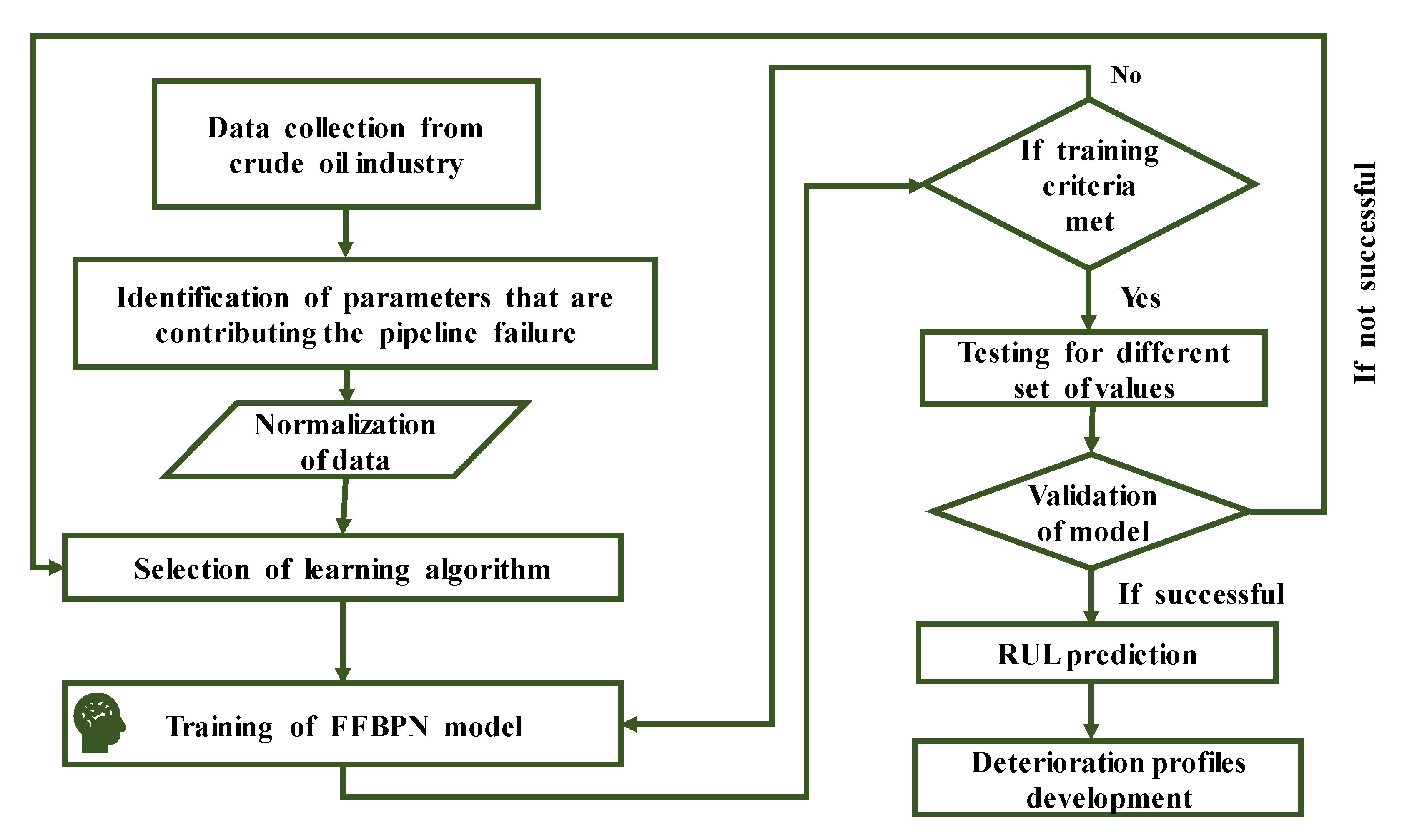
2. Proposed Feed Forward Back Propagation Network (FFBPN) Approach

The overall methodology is presented in Figure 1. The first step comprises of collecting the data from the crude oil industry. Six parameters were identified, based explicitly on the higher impact on the pipeline condition. The FFBPN technique was used for training a model which is the performance of two-way iterations. The first way includes the forward step computation of input weights and the second way is backward step computation for updating weights and calculating errors. The training data was normalized within the range of [0–1]. Seventy percent of collected data was used for training the model, whereas 30% of the data is divided equally for the testing and validation, respectively. Secondly, the model was trained based on Equation (1) until the criteria met [19].

$$x_k={\displaystyle \sum }_i^n{w}_{ki}{x}_i$$

(1)

where x_k is the variable’s new value, x_i is the variable’s initial value and w_ki is the neuron/variable’s weight link value. The activation function between the input and the hidden layer was ‘logsig‘, as indicated by Equation (2).

$$f\left(x\right)=1/\left(1+e^{-x}\right)$$

(2)

The purelin function was used as Equation (3) between the hidden layer and the output layer:

$$f\left(x\right)=x$$

(3)

Finally, the model was validated for its reliability with a new (unknown) data set and the results were found to be satisfactory. The justification for these stages is discussed in the results section.

2.1. Data Collection

The data was collected from the Sudan-based crude oil industry. The inspection team divided the pipeline into five sections, as the length of the pipeline was found to be large (1135.88 km).

Table 1. Characteristics of collected pipeline data.

Parameter	Unit
Max. Allowable Operating Pressure (MAOP)	97 (bar)
Product type	Waxy crude oil
Diameter	32 (inches)
Material	API 5L X 65/X 70
Length	1135.88 (km)
Nominal wall thickness	11.71 (mm)/18.91 (mm)
Design Factor	0.72
Assessment pressure	80 (bar)
Design pressure	100 (bar)
Inspection years	2009 and 2015

shows the details of the pipeline characteristics. The inspection was carried out at different time intervals on each segment. The fourth section of the pipeline, which had a length of 241.21 km, was found to have significant anomalies of internal metal loss and welding anomalies. Therefore, data from the fourth section was used during this study. Later the parameters of the fourth section were considered and normalized. Each parameter of this section had 85,519 reference points and the data was normalized, which is discussed in the further section in detail.

2.2. Impact of Critical Factors on Pipeline Condition

The questionnaire was sent to 90 professional experts in the oil and gas industry from various regions in Asia. Of the 90 given, 55 responded to the questionnaire; participants were provided with twelve different factors including cathodic protection, metal loss, welding anomalies, corrosion, product type, pressure flow, temperature difference, third party, crossings, wall thickness, environmental hazards and vibration. Participants were allowed to select multiple factors as responses without any restriction on the selection order.

Based on the opinion of experts, metal loss, corrosion, cathodic protection, product type and wall thickness were the parameters with maximum influence on the condition of oil and gas pipelines. It is important to mention here that the limited availability of periodic inspection data restricted the investigation of parameters affecting the condition of the pipeline. Thus, cathodic protection, corrosion and product type were identified as critical parameters for pipeline condition with a frequency percentage of 72.7%, 90.9% and 78.2%. The lack of available inspection data restricted the use of these parameters for model development. Nonetheless, during our survey results, the factors considered during this study presented a reasonably high significance. During survey results, metal loss, wall thickness, welding anomalies and pressure flow showed a frequency percentage of 81.8%, 70.9%, 58.2% and 29.1%. Thereby, the selection of input parameters used for model development was in accordance with survey responses. The parameters considered in this study were limited to metal loss anomalies, wall thickness, weld anomalies and pressure flow.

2.3. Parameters Considered for the Model Development

The six parameters including metal loss (length, width and depth), wall thickness, weld girth and pressure were considered from the data and given as inputs, and Estimated Repair Factor (ERF) is taken as output to develop the FFBPN model as shown in Figure 2. The model was developed in three stages, namely training, testing and validation, in which 70%, 15% and 15% of data were used, respectively. If the training criteria are met in the first stage, then the model proceeds to the test stage where it is tested to measure its performance for a given testing data sample values; otherwise, it is recalled for retraining in the first stage. The model is successfully developed and validated after the testing stage.

2.4. Data Normalization

The data was normalized using Equation (4). Six parameters were considered as inputs, namely metal loss anomalies (including length, width and depth), wall thickness, weld girth and pressure flow, and Estimated Repair Factor (ERF) as output. The metal loss feature’s safe working pressure (Ps) was calculated based on the remaining strength assessment method (ASME B31 G). The severity of metal loss features and need for repair action was determined, as shown in Figure 3, according to the ratio of safe pressure to assessment pressure (80 bar). The mathematical relationship of ERF is presented in Equation (5). Each variable that was considered in this work had 85,519 reference points. Thus, 6 × 85,519 values were considered as inputs, and 1 × 85,519 values were considered as outputs.

$$x_{new}=\frac{x-x_{min}}{x_{max}-x_{min}}$$

(4)

where x_new is a new value, x is an original value, x_max is a maximum value, and x_min is a minimum value of a specific parameter.

ERF = Assessment pressure/Safe working pressure

(5)

2.5. FFBPN Model Development

MATLAB^® 2018a was used to develop the FFBPN model. During the initial training stage, the FFBPN-based model is trained using the available historical data. If the model fails to meet expectations, it will allow the process to be re-propagated until it reaches the best requirement using the Levenberg-Marquardt (LM) backpropagation algorithm [20]. After completion of the model training, 15% of the data was used to validate the trained model at the validation stage. Once the accuracy was reached, the model was allowed for the test stage and tested with the remaining 15% of the data sets, and results were found to be accurate with the R² value reached close to 1.0. The network consists of three layers, i.e., input, hidden and output layers as shown in Figure 2. The proposed network was used with sigmoid function (tansig) in the hidden layer and the linear function (Purelin) in the output layer. The input layer receives the input signals from the other source; the role of the hidden layer is to transform the signals into something that the output signal can use in some way. The proposed neural network architecture with ‘tansig’ and ‘purelin’ functions is presented in Figure 4. This neural architecture is also called a multi-layer perceptron. The standard multilayer perceptrons are capable of approximating any quantifiable function to the desired accuracy rate [21].

The six parameters mentioned above have been used as inputs and ERF has been used as a target for the model development. Notably, the model was trained with a different number of neurons, out of which, 16 neurons gave the best predicted output and the selected number of data sets were sufficient to train, validate and test the model.

3. Results and Discussions

3.1. FFBPN Model Training

A FFBPN neural network has been developed to predict a crude oil pipeline’s life condition. Specific factors have been considered as inputs for model development as limited data were available. The model developed was trained on the basis of Equation (1) and the Levenberg-Marquardt backpropagation algorithm; the model has been later validated and tested by providing all possible data sets. The R² value has been predominantly changed as the number of hidden neurons was varied, starting from a minimum of 6 to a maximum of 20, as shown in Figure 5. The precise values of R² have also been presented along with the respective number of neurons. The Mean Square Error (MSE) values for each stage have been calculated using Equation (6) [22]

$$MSE=\frac{1}{2}{\displaystyle \sum }_{m=1}^n{\left(O_a-O_p\right)}^2$$

(6)

where MSE is the mean of error squares, O_a is the actual output and O_p is predicted output.

The accuracy of the developed model has been found to be highly sensitive to the number of hidden neurons.

Table 2. Values of Training, Testing, Validation and overall R² based on number of neurons.

No. of Neurons	Training		Validation		Testing		Overall R2
	MSE	R2	MSE	R2	MSE	R2
6	11.2354	0.9513	21.6136	0.9571	16.0711	0.7641	0.9372
7	10.0785	0.9609	60.7338	0.8935	19.8944	0.9463	0.9547
8	1.3699	0.9931	11.6083	0.7578	25.8974	0.8624	0.9645
9	3.5939	0.9880	20.6453	0.9796	24.8692	0.1707	0.9604
10	19.5869	0.9252	10.8580	0.3483	14.4814	0.8686	0.9045
11	4.9530	0.9768	10.9544	0.8166	30.9652	0.8871	0.9430
12	3.7410	0.9824	10.6335	0.8287	71.8311	0.6975	0.9215
13	2.3421	0.9780	0.0464	0.9787	56.0370	0.9144	0.9376
14	2.4702	0.9867	10.3475	0.9409	7.3257	0.9091	0.9749
15	0.9471	0.9945	20.8847	0.9022	13.8276	0.9275	0.9665
16	0.0894	0.9973	0.1046	0.9970	0.0783	0.9977	0.9998
17	1.6581	0.9908	10.9430	0.9465	26.9734	0.8224	0.9622
18	1.7737	0.9887	9.9706	0.9658	66.2021	0.6006	0.9276
19	2.0126	0.9876	16.7679	0.9224	13.1037	0.9619	0.9677
20	2.3673	0.9848	35.6957	0.8710	20.8974	0.9494	0.9509

shows the overall R² values against the respective number of hidden neurons, with MSE and R² values, in all stages. The best network architecture was found to be [6 × 16 × 1]. Variations in R² and MSE values along typical ANN stages with 16 hidden neurons are illustrated in Figure 6. The overall R² values are found to be consistent with the number of neurons ranging from 12 to 18, the detailed results obtained against these neurons are presented here. During the selection of optimum network structure, the error for the existing state of the neural network must be assessed constantly. This needs the selection of an error function, conventionally called a loss function, which can be used to estimate the loss of the model, so that the weights can be updated to reduce the loss on the next evaluation. In this study, MSE has been used as loss function to compute the performance of neural network.

The variations in the value of MSE and R² over the number of hidden neurons are clearly represented in Figure 6. Notably, all stages have R² values close to 1.0 and MSE values close to 0, with 16 hidden neurons shown in the Figure 6 by a dotted line.

Figure 7 represents the summary of R² plots in training, testing and validation stages during the training process. For the training data set, an overall R² value of 0.9998 has been obtained. The neural network was trained and validated using available historical data set to develop a robust model with the finest predicted accuracy of the output. The results have been found to be satisfactory, as the overall R² value is close to 1.0. Notably, the R² value in each stage is close to 1.0, i.e., 0.9997, 0.9999 and 0.9999 for training, validation and testing stages, respectively, as shown in Figure 7.

Figure 8 consists of a plot between Mean Squared Error (MSE) and Epochs. The best validation performance was obtained at epoch 528, with validation plot reaching its minimum MSE value of 0.12456.

3.2. FFBPN Model Testing

Figure 9 represents the plot with R² value of 0.9978 obtained during the testing of model. The developed neural network model was applied to the different data set to test the predicted accuracy of the output and the results were found to be satisfactory as the R² value is close to 1.

In addition, a new sample data set has been selected from actual historical data from 2009 and 2015. The values of metal loss, wall thickness, pressure and weld girth have been later used as input to predict the ERF value using the FFBPN model. Figure 10 illustrates the plot between the actual ERF and the predicted ERF values. The plot indicates reasonable agreement with Root Mean Square Error (RMSE) and Mean Absolute Percent Error (MAPE) values of 0.025149 and 0.025263, respectively, between actual and predicted data sets.

3.3. Metal Loss Growth Rate Calculation Results

The severity of growth in metal loss leads to the degradation of a pipeline. Therefore, it is necessary to be careful to eliminate a pipeline’s catastrophic failures. In total, 85,519 metal loss anomalies were recorded from the historical data. The rate of growth in metal loss is calculated using Equation (7)

$$R_{ML}=\frac{D_2-D_1}{Ins. Dt{.}_1-Ins. Dt{.}_2}$$

(7)

where R_ML is ML growth rate, mm/yr.; D₁ is ML depth level in the first inspection, mm; D₂ is ML depth level in the second inspection, mm; Ins. Dt₁ is first inspection date, yr. and Ins. Dt₂ is the second date of inspection, yr.

The metal loss growth rates are acquired from historical inspection data.

Table 3. Metal loss growth rate results.

Range	Metal Loss Depth Level	Depth Recorded in 2009 Inspection (%wt)	Depth Recorded in 2015 Inspection (%wt)	Max. Growth Rate (mm/yr)
Optimistic	0%wt ≤ D < 10%wt	0	9	0.27
Average	10%wt ≤ D < 20%wt	0	19	0.58
Pessimistic	30%wt ≤ D < 40%wt	0	30	0.91

presents the calculated results for three metal loss rates, i.e., pessimistic, average and optimistic rates, which provide a confidence interval range for the remaining useful life (RUL) of the pipeline.

3.4. Remaining Useful Life Calculation Results

After the metal loss growth rates are calculated and current ERF is predicted from FFBPN model, they are used to predict the RUL of the pipeline. The trajectory of deterioration is extended from predicted ERF value at time instant t_c, by combining it with the metal loss growth rates. The time at which the trajectory hits the threshold ERF value is termed as failure time t_f. The RUL can be calculated by subtracting both the times as given in Equation (8) (Ahsan et al., 2019).

$$\mathit{RUL}=t_f-t_c$$

(8)

For this research, three different deterioration ranges were used to predict crude oil pipeline RUL such as (i) optimistic, (ii) average, and (iii) pessimistic.

Table 4. Predicted Remaining Useful Life for crude oil pipeline.

	Optimistic	Average	Pessimistic
Rate	0.27	0.58	0.91
Predicted RUL	26 years	14 years	10 years

presents the predicted RUL for these three rates.

The predicted RUL may help pipeline technicians take all the necessary actions and plan the maintenance accordingly, which may reduce the production losses of the oil and gas pipeline industries.

3.5. Sensitivity Analysis

It is necessary to recognize evidently about the interrelationships between the factors considered and the pipeline condition; for that purpose, the correlation analysis suing Microsoft Excel software is carried out to identify the individual influence on the life of pipeline condition. The developed model is put through sensitivity analysis to discuss its sensitivity to changes in the factor values. In other words, the developed model is performed to examine how the uncertainty in inputs could affect the output. A contribution percent of each factor considered for this study is given according to the severe impact on pipeline’s life, as shown in

Table 5. Relative Contribution of individual factors.

Individual Factor	Relative Percentage (%)
Length	10.72638761
Width	8.534201257
Depth	2.856189363
Wall thickness	37.2331322
Pressure	40.5805349
Weld Girth	0.069554677
Total	100

.

It is important to know the effect of each individual factor on the pipeline condition. For this reason, deterioration profiles have been generated, as shown in Figure 11. The value of one selected factor has been varied while the other factors have been kept constant with their respective average values. Later, the model has been allowed to predict the new values, the variations that have been observed in the new prediction pipeline condition is because of the factor that is varied, and other factor values kept the same at their average values. The profiles have been generated for each factor following the same process. The summary of all deterioration profiles for all factors are shown graphically in Figure 11. It is found that the pressure has major negative affect on pipeline condition, and weld girth has the minor negative affect on pipeline condition.

A comparison test for developed FFBPN model is performed with earlier approaches such as Regression analysis, ANN and Fuzzy logic techniques for its robustness.

Table 6. Performance Comparison of FFBPN with previous studies.

Technique	R2	RMSE	Validation Accuracy
FFBPN	0.9998	0.02514	99%
ANN [23]	0.9064	0.08	92%
Regression [24]	0.9940	0.015	96%
Fuzzy Logic [25]	N/A	0.07	83%
ANN [12]	0.9959	0.012	97%

summarizes the comparison results of the proposed FFBPN model with other previous approaches in terms of R², RMSE values and validation accuracies. It is observed that the proposed FFBPN technique is a good robust performance indicator in terms of pipeline condition prediction. The results for earlier approaches are found to be acceptable and close to 1.0. However, the results show that FFBPN showed slightly better performance than previous approaches, with the R², RMSE value and validation accuracy of 0.9998, 0.02514 and 99%, respectively, as shown in Table 6.

4. Conclusions

• The prediction model to assess the condition of the crude oil pipeline was developed using the Back Propagation Neural Network technique focused on specific factors such as metal loss anomalies (across length, width and depth), wall thickness, weld girth and pressure flow.
• The results of FFBPN model found to be satisfactory based on an R² value of 0.9998. The predicted output accuracy was found to be highly dependent on the number of neurons.
• The model was tested with a new data set and the results were found to be good, with the R² value of 0.99.
• The FFBPN model was validated using a new sample data and the results were found to be accurate with Root Mean Square Error (RMSE) and Mean Absolute Percentage Error (MAPE) values of 0.02514 and 0.02526, respectively.
• The deterioration curves were generated to know the effect of each factor selected on the pipeline condition; it was found that pressure has a major negative effect on pipeline condition and weld girth has a minor negative effect on pipeline condition.
• The proposed FFBPN was validated with other published models for its robustness and it was found that FFBPN performed better than the previous approaches based on R² and RMSE.
• In terms of maintenance scheduling, the proposed approach will be beneficial. The developed model can be applied to real-time data to help pipeline operators take the necessary actions to prevent product losses in the oil and gas pipeline industries.

References

1. Kennedy, J.L. Oil and Gas Pipeline Fundamentals; Pennwell Books: Tulsa, OK, USA, 1993. [Google Scholar]
2. El-Abbasy, M.S.; Senouci, A.; Zayed, T.; Mosleh, F. A condition assessment model for oil and gas pipelines using integrated simulation and analytic network process. Struct. Infrastruct. Eng. 2015, 11, 263–281. [Google Scholar] [CrossRef]
3. Shabarchin, O.; Tesfamariam, S. Internal corrosion hazard assessment of oil & gas pipelines using Bayesian belief network model. J. Loss Prev. Process Ind. 2016, 40, 479–495. [Google Scholar]
4. Dey, P.K.; Ogunlana, S.O.; Naksuksakul, S. Risk-based maintenance model for offshore oil and gas pipelines: A case study. J. Qual. Maint. Eng. 2004, 10, 169–183. [Google Scholar] [CrossRef]
5. Jinhai, L.; Huaguang, Z.; Jian, F.; Heng, Y. A new fault detection and diagnosis method for oil pipeline based on rough set and neural network. In Proceedings of the International Symposium on Neural Networks, Nanjing, China, 3–7 June 2007; pp. 561–569. [Google Scholar]
6. Peng, X.-Y.; Zhang, P.; Chen, L.-Q. Long-distance oil/gas pipeline failure rate prediction based on fuzzy neural network model. In Proceedings of the 2009 WRI World Congress on Computer Science and Information Engineering, Angeles, CA, USA, 31 March–2 April 2009; pp. 651–655. [Google Scholar]
7. Tabesh, M.; Soltani, J.; Farmani, R.; Savic, D. Assessing pipe failure rate and mechanical reliability of water distribution networks using data-driven modeling. J. Hydroinform. 2009, 11, 1–17. [Google Scholar] [CrossRef]
8. Bersani, C.; Citro, L.; Gagliardi, R.V.; Sacile, R.; Tomasoni, A.M. Accident Occurrance Evaluation in the Pipeline Transport of Dangerous Goods. Chem. Eng. Trans. 2010, 249–254. [Google Scholar] [CrossRef]
9. Noor, N.; Yahaya, N.; Ozman, N.; Othman, S. The forecasting residual life of corroding pipeline based on semi-probabilistic method. J. Civ. Eng. Sci. Technol. 2010, 1, 1–6. [Google Scholar]
10. Dawotola, A.W.; Van Gelder, P.; Vrijling, J. Decision analysis framework for risk management of crude oil pipeline system. Adv. Decis. Sci. 2011, 2011, 456824. [Google Scholar] [CrossRef] [Green Version]
11. Ahmadi, M.A.; Ebadi, M.; Shokrollahi, A.; Majidi, S.M.J. Evolving artificial neural network and imperialist competitive algorithm for prediction oil flow rate of the reservoir. Appl. Soft Comput. 2013, 13, 1085–1098. [Google Scholar] [CrossRef]
12. El-Abbasy, M.S.; Senouci, A.; Zayed, T.; Mirahadi, F.; Parvizsedghy, L. Artificial neural network models for predicting condition of offshore oil and gas pipelines. Autom. Constr. 2014, 45, 50–65. [Google Scholar] [CrossRef]
13. Szoplik, J. Forecasting of natural gas consumption with artificial neural networks. Energy 2015, 85, 208–220. [Google Scholar] [CrossRef]
14. Ayegba, P.; Abdulkadir, M.; Hernandez-Perez, V.; Lowndes, I.; Azzopardi, B.J. Applications of artificial neural network (ANN) method for performance prediction of the effect of a vertical 90 bend on an air–silicone oil flow. J. Taiwan Inst. Chem. Eng. 2017, 74, 59–64. [Google Scholar] [CrossRef]
15. Ghumman, A.R.; Ahmad, S.; Hashmi, H.N. Performance assessment of artificial neural networks and support vector regression models for stream flow predictions. Environ. Monit. Assess. 2018, 190, 704. [Google Scholar]
16. Zabihi, R.; Mowla, D.; Karami, H.R. Artificial intelligence approach to predict drag reduction in crude oil pipelines. J. Pet. Sci. Eng. 2019, 178, 586–593. [Google Scholar] [CrossRef]
17. Tan, Z.X.; Thambiratnam, D.P.; Chan, T.H.; Gordan, M.; Abdul Razak, H. Damage detection in steel-concrete composite bridge using vibration characteristics and artificial neural network. Struct. Infrastruct. Eng. 2019, 1–15. [Google Scholar] [CrossRef]
18. Aguilar, V.; Sandoval, C.; Adam, J.M.; Garzón-Roca, J.; Valdebenito, G. Prediction of the shear strength of reinforced masonry walls using a large experimental database and artificial neural networks. Struct. Infrastruct. Eng. 2016, 12, 1661–1674. [Google Scholar] [CrossRef]
19. Basha, S.N.; Rao, P.S. A Simulated Model for Assesing the Line Condition of Onshore Pipelines. In Proceedings of the MATEC Web of Conferences, Perak, Malaysia, 18–19 September 2018. [Google Scholar]
20. Moayedi, H.; Aghel, B.; Vaferi, B.; Foong, L.K.; Bui, D.T. The feasibility of Levenberg–Marquardt algorithm combined with imperialist competitive computational method predicting drag reduction in crude oil pipelines. J. Pet. Sci. Eng. 2020, 185, 106634. [Google Scholar] [CrossRef]
21. Taqvi, S.A.; Tufa, L.D.; Zabiri, H.; Maulud, A.S.; Uddin, F. Fault detection in distillation column using NARX neural network. Neural Comput. Appl. 2018, 1–17. [Google Scholar] [CrossRef]
22. Sarbayev, M.; Yang, M.; Wang, H. Risk assessment of process systems by mapping fault tree into artificial neural network. J. Loss Prev. Process Ind. 2019, 60, 203–212. [Google Scholar] [CrossRef]
23. Senouci, A.; Elabbasy, M.; Elwakil, E.; Abdrabou, B.; Zayed, T. A model for predicting failure of oil pipelines. Struct. Infrastruct. Eng. 2014, 10, 375–387. [Google Scholar] [CrossRef]
24. El-Abbasy, M.S.; Senouci, A.; Zayed, T.; Mirahadi, F.; Parvizsedghy, L. Condition prediction models for oil and gas pipelines using regression analysis. J. Constr. Eng. Manag. 2014, 140, 04014013. [Google Scholar] [CrossRef]
25. Senouci, A.; El-Abbasy, M.S.; Zayed, T. Fuzzy-based model for predicting failure of oil pipelines. J. Infrastruct. Syst. 2014, 20, 04014018. [Google Scholar] [CrossRef]
Figure 1. FFBPN approach workflow.
Processes 08 00661 g001
Figure 2. Proposed Neural Network architecture.
Processes 08 00661 g002
Figure 3. Flowchart for determination of Estimated Repair Factor.
Processes 08 00661 g003
Figure 4. Proposed network architecture with functions.
Processes 08 00661 g004
Figure 5. Variation of R2 value over number of hidden neurons.
Processes 08 00661 g005
Figure 6. Variations in MSE and R2 values with number of neurons.
Processes 08 00661 g006
Figure 7. Training, Testing, Validation and overall R2 = 0.9998 obtained for training data set.
Processes 08 00661 g007
Figure 8. Best validation performance plot.
Processes 08 00661 g008
Figure 9. Performance of model on Testing data set based on R2.
Processes 08 00661 g009
Figure 10. Plot for actual ERF vs predicted ERF.
Processes 08 00661 g010
Figure 11. Deterioration profiles of factors.
Processes 08 00661 g011