Assessment and Prediction of Complex Industrial Steam Network Operation by Combined Thermo-Hydrodynamic Modeling

Abstract

Steam network operation stability and reliability is vital for any industrial branch. A combined steam network model comprising a balance and a coupled thermo-hydrodynamic model, including seasonal variations impact and system specificities, is presented. A balance model can readily be used by a refinery’s operators. The thermo-hydrodynamic model identifies system bottlenecks and cold spots and evaluates proposed operation and investment measures including heat loss reduction. A three-pressure levels refinery steam network served for model testing and validation. Balance model results reveal significant misbalance in steam production and consumption, reaching 30.5% in the low-pressure steam system, and heat balance differences in the range of 9.2% to 29.5% on individual pressure levels, attributable both to flow measurement accuracy issues and to heat losses. The thermo-hydrodynamic model results differ from the measured steam parameters by less than 5% (temperature) and by less than 4% (pressure), respectively, with the estimated operational insulation heat conductivity exceeding 0.08 W/m/K. Its comparison with that of 0.03 W/m/K for dry insulation material yields the need for pipelines re-insulation and a partial revamp of the steam network. The model is sufficiently general for any type of industry, pursuing the goal of cleaner and energy-efficient steam transport and consumption.

1. Introduction

Water steam belongs to the most extensively used energetic media. Already in 2006 the share of energy consumption in the form of water steam represented up to 40% of all energetic media used in industry. In the refining industry, up to 28% of total energy consumption belongs to water steam production [1]. A system with a central steam source (combined heat and power (CHP) unit) with decentralized secondary ones is preferred, with steam being transported to its consumers through complicated pipe networks with total length reaching up several tens to hundreds of kilometers within one plant [2]. With such transport distances, it is difficult to keep the steam network in a stable state and to secure desired steam quality to all consumers under all conditions. Fluctuations of steam parameters may affect production units in the refinery. Stable and effective operation of steam networks also leads to a reduction of steam losses to the environment and reduced operational costs for the whole enterprise [3].

Several papers have been published regarding the design of different utility systems and their optimization. Nishio et al. [4] used a simple linear programming (LP) algorithm for turbine allocation. Mixed-integer linear programming (MILP) and mixed-integer non-linear programming (MINLP) has become very popular since the 1980s [5,6] and was used in different tasks such as simulation and optimization of utility systems leading to significant cost savings achievement [7] and other benefits, such as maximizing the total power generation of steam turbines network [8]. A simple mathematical model based only on mass and heat balance, which enabled switching between different production loads and switching between electro- and steam drive, was applied in a refinery. It led to the realization of new projects within the steam network [9]. Mass and energy balances were adopted as the base for another MILP model that required solving linear equations to achieve the reduction of operational costs and steam production in a petrochemical company, which produces electric energy and steam by co-generation system [10]. The MILP method can also be applied to determine the optimal steam network operation, benefits of investments in boilers and cogeneration units or to optimize their operation [11,12]. In another paper, a MILP model targeting minimum flowrate and designing the steam network simultaneously was used [13].

Minimization of steam costs and power generation in a petrochemical company as a result of a MILP-based mathematical model brought the potential of saving a 46 t/h of generation in steam boilers and reduction of 6 MW of electric power consumption [14]. A MILP model considering unit costs of different kinds of energies can provide the energy plant operators recommendations for use of an optimal energy consumption of composition, which results in the energy expenses minimization [15].

Mass and energy balances were adopted as the base for another mixed-integer non-linear programming (MINLP) mathematical model of steam turbine network, which consisted of more complicated systems of non-linear Equations [16]. The comparison of results obtained by this model to the real field data proved the mean relative error less than 1.18%. Other examples of using MINLP include retrofit and optimization of total site steam distribution networks [17,18] or optimization of whole industrial sites [19].

Enhanced and more accurate mathematical models include hydrodynamic equations. Luo et al. in their work proposed relatively simple mathematical model and refer to previous models of other authors. Steam flow velocity in each pipe segment can be more precisely estimated only by a combination of hydrodynamic equations and heat balance [20]. Tian applied laws of mass, momentum and energy conservation to solve steam flow equations [21]. Recent studies reflect the non-linear programming in so-called “mass, heat and work exchange networks” modeling [22,23,24] with simultaneous synthesis, design and operation optimization of the energy management of extensive industrial sites.

Rigorous mathematical modeling includes models that manage handling multiphase flow calculations [25] but solving of ordinary differential equations (ODE) [26], partial differential equations (PDE) [27] or differential-algebraic equations (DAE) [28,29] is necessary as well. A mathematical model predicting the amount of condensate and considering condensate losses was proposed in the past and allows application on single pipes or whole steam networks [21,30]. It consists of differential equations based on mass and energy conservation laws. In the case of a whole network in a large Chinese steel plant, very good results were obtained with relative errors for mass flow, pressure and temperature calculations of 1.99%, 1.97% and 2.2%, respectively. By optimizing the back-pressure/condensing turbines operation and steam imports in a German refinery, the system achieved an average 2.75 mil. USD/year [31] cost savings. It is useful for data reconciliation, steam balancing, marginal steam value calculation and “what if” studies preparation.

Artificial neural networks (ANN) offer enhanced possibilities in mathematical modeling [32]. In recent years ANN were successfully used to optimize the steam turbine network [33,34] and combined heat and power system [35] or to develop a steam turbine model for online monitoring purposes [36] or to develop an online monitoring system for the steam process of a combined heat and power plant [32]. Other fields of application include waste heat recovery [2,37] while paying heed to electricity cogeneration [38,39], or steam quality control modeling and prediction [40,41].

The literature survey performed allows for formulation of the following observations forming the knowledge and experience gap this paper has the ambition to fill:

• Despite the documented extensive research in steam networks modeling, most of presented models deal with steam network optimization just as a part of a bigger optimization scheme [31,33].
• Detailed system specificities and topology are seldom considered which might lead to system operation analysis oversimplification [17,18].
• Seasonal ambient air temperature variations impact on system operation is rarely considered which might prevent the performed study to reveal the season-related system bottlenecks [21].
• Most models analyze the steam system under one certain or a few selected loads (transported steam amounts and transport directions) which does not allow for a rigorous assessment of problematic operation situations and troublesome spots in the steam network [34,36].
• Though system operation change/improvement projects (re-insulation, new pipelines commissioning, impact of new production units on system operation) are commonly considered and tested, the testing procedure frequently does not consider all possible network operational states, or, at least, all those states that were recorded in the past [14,19]. This in turn limits the testing ability to identify system bottlenecks possibly resulting from improvement project implementation.

The aim of the presented paper was to focus directly on the issues discussed above, namely closely on the steam system itself, incorporating its specificities and the impact of seasonal variations, thus providing an alternative and more realistic point of view on the steam system’s operation limits. More specifically, the main aim can be split into the following:

• Creation of a mathematical model that would be able to detect and to predict troublesome spots formation within the steam networks with increased possibility of cold spots or bottlenecks occurrence.
• Its testing on a real complex steam system of a refinery; its use to reveal particular operation problems and limits in the existing system.
• The use of the developed model to predict the impact of planned investments in the refinery on the operation stability of the steam system, considering seasonal system operation changes.
• Proposal and simulation of the system changes for its operation improvement.

Firstly, mass and heat balances were performed for each individual steam pipeline followed by a simple balance model calculating steam flow velocities in each pipe segment to assess the possibility of “cold spot” or “bottleneck” formation. Secondly, a combined thermo-hydrodynamic model based on hydrodynamic and heat-transfer equations was created that allows comparing calculated values of steam temperature and pressure to the real field data. This model, after validation, was used for assessment of proposed changes within the steam network.

2. Problem Description

The SLOVNAFT company is a complex oil refinery designed and built in the 1960s. Gradual development of equipment and technology as well as improved heat recovery meant that the operational parameters of steam networks are significantly different than they were designed for originally. The risk of cold spots occurrence in the steam mains increases especially due to the steadily rising share of steam produced in local steam sources. Non-optimal operation of steam networks leads to significant economic losses. Other facts contribute to this state as well:

• The “safe” layout of the refinery—all operational units in the refinery are located relatively far apart. Thus, there is a need to transport steam over long distances, leading to increased heat losses to the surroundings.
• Several steam-drives at the SLOVNAFT refinery have been switched to electro-drives, except important devices, that are still being driven by steam turbines as a safety measure. Switching between electro- and steam-drives is important not just from the economical point of view but allows the steam balance to be influenced. With too many devices switched to electro-drives (which is economically effective), steam supply from a CHP unit would drop significantly and result in steam condensation in pipelines. Therefore, the economics is not the only decision-making factor. Operational safety is important as well.
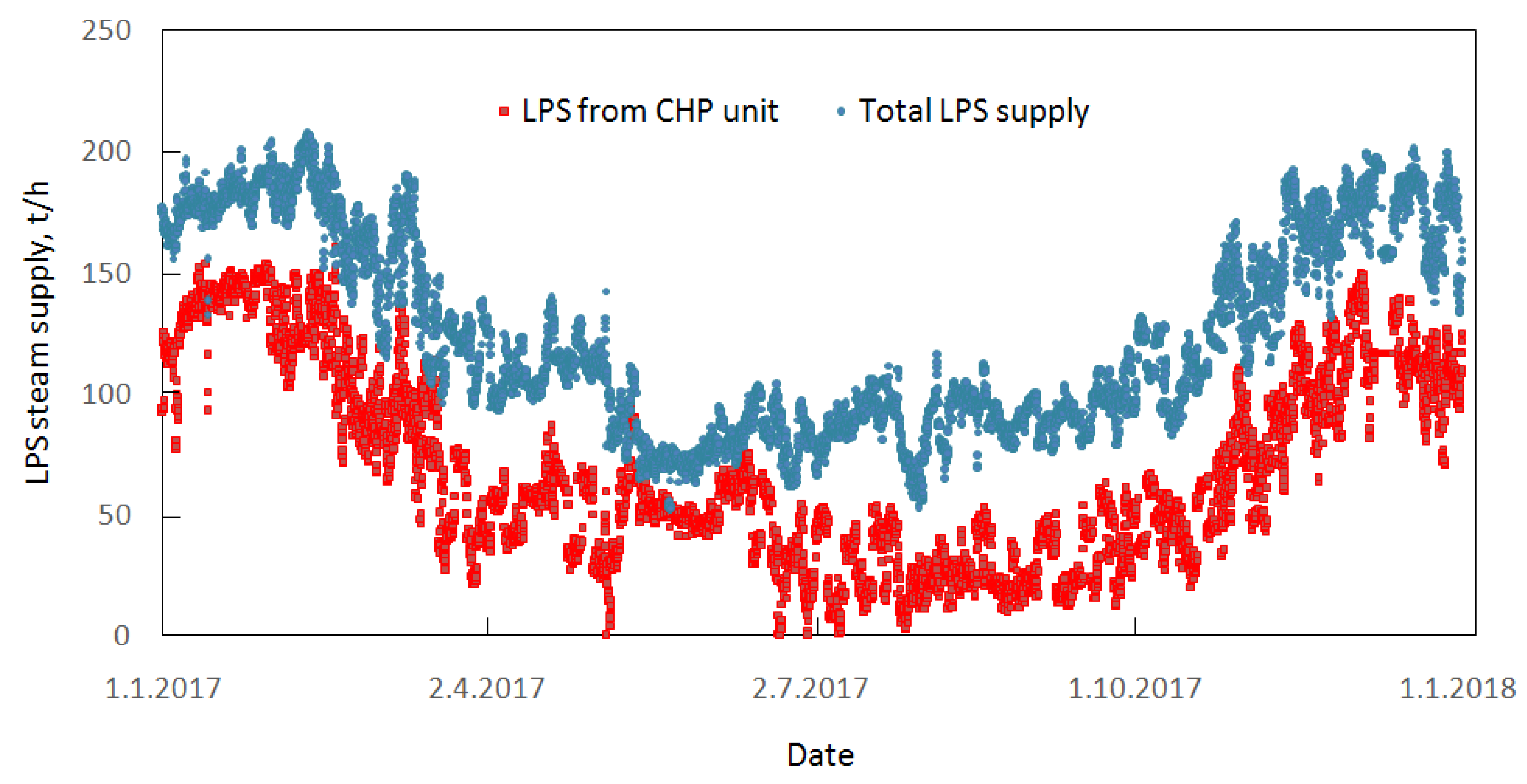
• Seasonal impact on operational state of steam networks. Summer months in particular are problematic due to excessive steam supply from secondary energy sources (SEC, all steam supplying units except CHP). The aforementioned switching between electro- and steam-drives reduces the possibilities of its utilization by production units. Steam excess is disposed of, by its condensation in air condensers, or, in worst situations, by its exhaust to the atmosphere.

Operation of steam networks is regulated by an internal directive, whose most important goals are:

• Keeping balance between steam production and its consumption.
• Maximal utilization of steam produced in CHP unit and secondary heat sources.
• Maximization of waste heat utilization in the form of low-pressure steam (LPS) produced at production units.
• Preserving steam quality parameters in desired intervals.
• Elimination of cold spots in steam networks.
• Utilization of electro-drives.
• Minimization of steam let-downs in CHP unit and other production units.

The occurrence of cold spots has the potential to exhibit damaging effect on several steam utilizing devices such as steam turbines. Condensate droplets are carried by flowing steam into turbines and due to their high velocity, turbine blades could get seriously damaged. Therefore, increased attention is paid to particular pipeline sections, deemed as potential cold spots, mainly based on historical data and previous experiences. Steam networks are managed the way the temperature is always higher than a certain value at these locations.

This method is very simple and effective, but has a major disadvantage: This way, new possible cold spots or bottlenecks cannot be detected in advance. This is a motivation for development of a mathematical model of steam networks able to overcome it.

The applied study method includes the following:

• Creation of mathematical models of steam networks and their application in the refinery on all pressure levels based on available operation data, visual controls and plant layouts.
• Mass and heat balances setup in order to determine current operational state of steam networks in the refinery.
• Confronting the simulation results with measured values of operational data to identify incorrect local measurement tools (steam pressure, temperature and mass flow).
• Assessment of troublesome spots formation risk in terms of low or very high steam flow velocity within individual sections of steam networks.
• Reviewing the impact of proposed projects within steam networks on its stability by a mathematical model expressed as steam temperature differences at individual steam-delivery points.
• Suitable measures proposal aimed at an improvement in the operational state of steam networks and the associated operating costs reduction.

3. Model Formulation

3.1. Operational Data Analysis

Three steam networks of different pressure level (low-pressure steam (LS); middle-pressure steam (MS); high-pressure steam (HS)) are operated in the refinery. The total length of all steam pipes reaches up to 60 km and there are 27, 20 and 18 active production units respectively connected to each steam pressure level. The average share of steam amount supplied by local steam sources to the total steam supply reaches up to 60% in the case of the HS network.

Steam flows and steam amounts being consumed or supplied in standard operational modes by individual production units as well as maximal steam flows through individual pipeline sections needed to be determined using past operational data. It was necessary to choose data corresponding to standard operational mode and sort/exclude data corresponding to planned or unplanned technical shutdowns and process data measurement failure.

Analyzed operational data included steam mass flows, temperatures and pressures. Based on values of steam temperature and pressure, the quality of steam (i.e., superheated/saturated/wet steam) can be determined. Moreover, by combination of steam pressure and the Antoine equation, the boiling point and superheating can be determined.

Finally, potentially incorrect values were identified and corrected or removed by detailed analysis of an extensive set of field data. Errors in the set of values can in our experience be caused by measurement failure, signal transmission error, improper placement of the measurement tool, a systematically different method of measuring, or exceeding the measuring scale.

To identify potentially incorrect values of raw process data, both simple logic and authors’ industrial experience obtained in previous practice were exploited. Negative process values (of mass flows, temperature and pressure) were treated as follows: The decision for a correction method was always made according to a timespan of such data failure. In case of a timespan shorter than 24 h, negative values have been replaced by the weighted arithmetic mean of the values observed during 24 h before the measurement failure. In a case that such failure persisted for more than 24 h, steam import or export were estimated using unit feed and specific steam consumption or production obtained from the unit′s past operation. The same approach was used in case of data failure accompanied by an error messages “No good data for calculation”, that were probably the most often occurring issues we had to deal with. Rarely, in the case of steam flows, we observed unit of measurement switch from t/h to kg/h and vice versa. Such values were manually transformed to the original unit of measurement, i.e., they were divided or multiplied by 1000.

3.2. Balance Model

The balance model was designed for real time monitoring purposes. In fact, the balance model is as simple as possible, thus shortening the calculation time and reducing hardware requirements and enabling its use by steam network operators.

The input data for the balance model comprise the following:

• Steam flows at individual production units (import, export or both, since some production units may act like steam importer and exporter at the same steam pressure level).
• Steam temperature and pressure at individual production units.
• Steam pipeline characteristics (lengths and diameters of individual pipe sections).

The input data were represented by the time-weighted hourly average values of measured field data measured during the whole year 2017. Thus, 8760 data sets containing 106, 68 and 81 measured values corresponding to high-pressure, middle-pressure and low-pressure steam (HPS, MPS and LPS), respectively, were processed. Prior to simulation, all data were analyzed and filtered if necessary (Section 3.1) to obtain reliable results.

The simulation schemes were prepared according to pipeline dimensions and existing technical drawings of the plant to preserve its layout as much as possible. A simplified scheme of HPS network is shown in Figure 1.

Specific enthalpy of steam for the purpose of heat balance was calculated by the IAPWS-IF97 method [42] that is considered to be a standard for steam enthalpy calculation published in 1997 by the International Association for the Property of Water and Steam. The specific steam volume was determined by method IAPWS-IF97 as well and it was used for steam flow velocity calculation.

The output data of the balance model are the following:

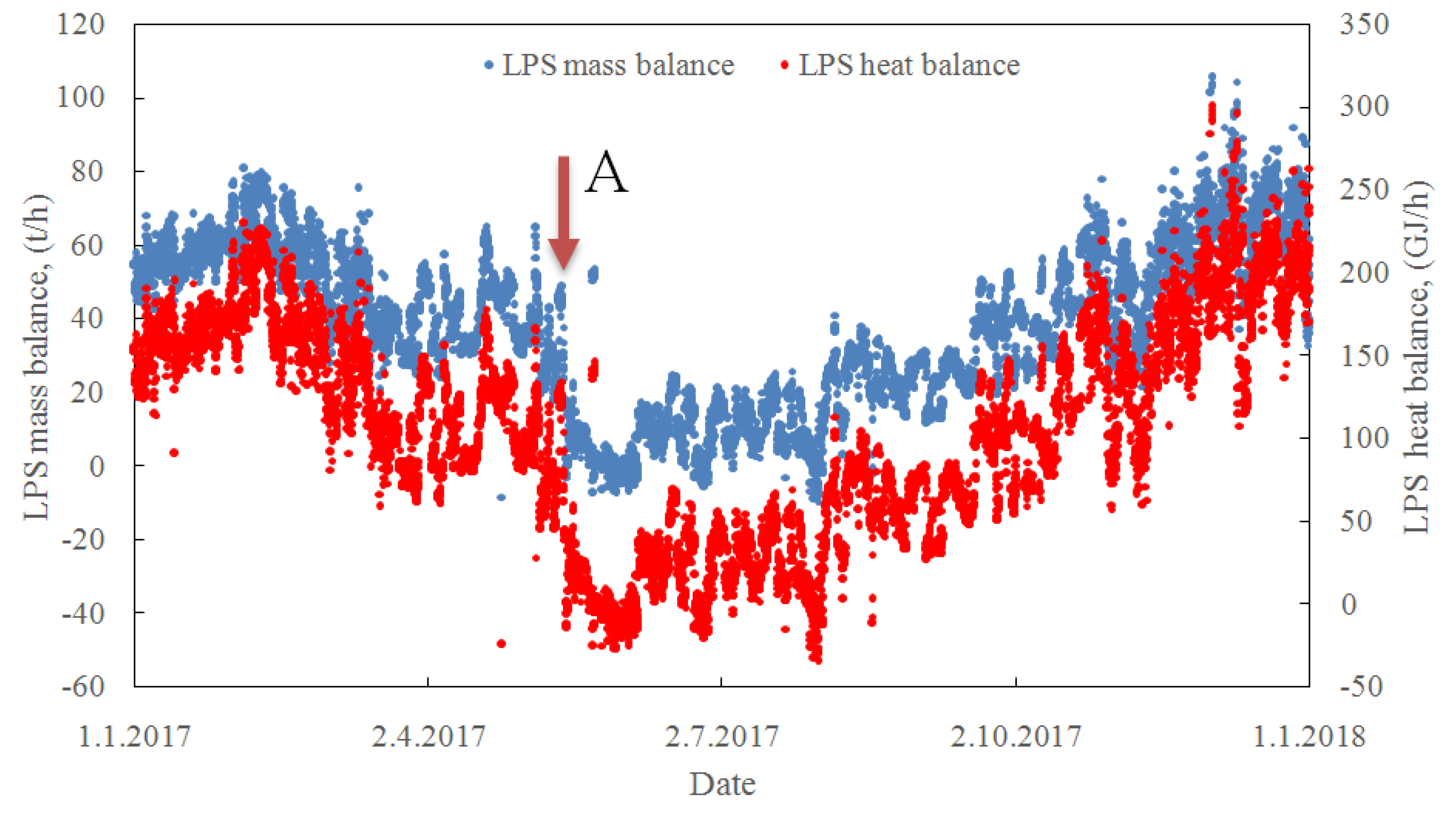
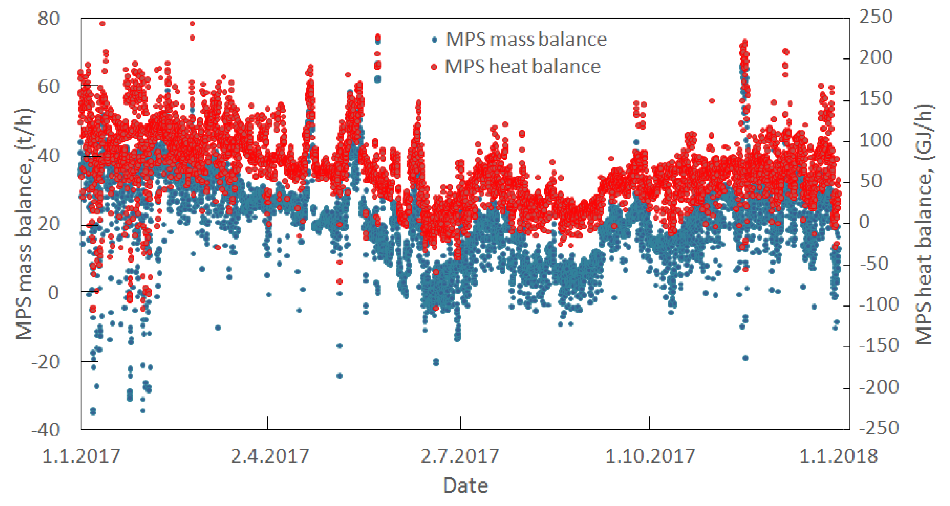
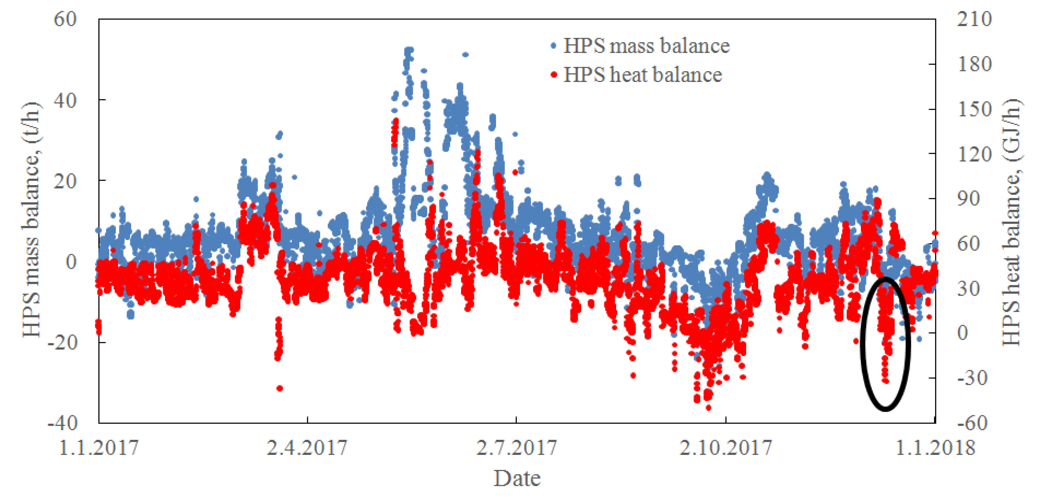
• Steam mass balance difference (i.e., the difference between steam mass supplied and consumed within the steam network).
• Steam heat balance difference (i.e., the difference between the heat supplied and consumed within the steam network in the form of steam).
• Steam flow velocities in individual pipe segments calculated according to steam mass flows in these pipe segments.

Based on the output data the overall technical state of steam networks as well as the economic impact of this state was evaluated. It was possible to assess the existence of cold spots as well as bottlenecks based on steam flow velocities w calculated in individual pipe sections by Equation (1), where $\dot{\mathrm{m}}$ represents the steam mass flow, v the specific volume of steam and D_in is the internal diameter of that pipe section.

$$\mathrm{w}=\frac{4\dot{\mathrm{m}}\mathrm{v}}{\mathsf{\pi }{\mathrm{D}}_{\mathrm{i}\mathrm{n}}^2}$$

(1)

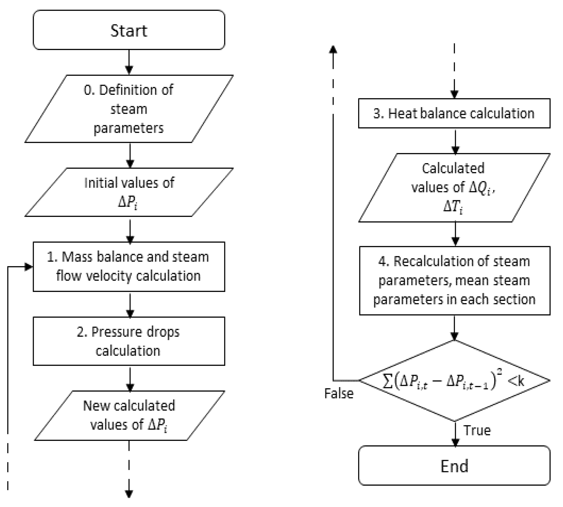
3.3. Combined Thermo-Hydrodynamic Model

This model was created in a commercial chemical modeling software environment, able to perform simulations of single pipes as well as complicated pipe networks. Other important features are:

• Simulation of single—or multiphase flow pressure drop with possible selection of calculation method.
• Heat-transfer calculation including outside weather conditions or physical properties of pipes.
• Calculation of profiles of different physical properties in pipe sections.

It is possible to perform simulations from single pipe segments to complex pipe networks. Each pipe segment can be divided into multiple sections with different properties (diameter, material, roughness, …). Number and types of fittings can be specified as well for pressure drop calculation.

This model is built to calculate temperature and pressure of outlet streams, while their mass flows are defined by the user. The inlet streams must be specified by combination of at least three input parameters: inlet pressure, temperature and molar/mass flow.

3.3.1. Pressure Drop Calculation

The used software works with many fluid flow pressure drop correlations. There are many empirical as well as mechanistic correlations, developed due to the calculation of pressure drop in wellbores or crude oil transport. Under common operation conditions, only superheated steam should be present in steam pipelines, but based on experience, saturated steam or even two-phase flow occurs on spots with lower steam flows. Therefore, we chose Beggs and Brill (1979) [43], which is the most widely used and most reliable fluid flow pressure drop correlation in industry suitable for two-phase flow simulations.

All pipe segments require definition of their properties, which are necessary for pressure drop calculation:

• Length;
• Inner diameter and outer diameter or tube wall thickness;
• Construction material (and its roughness);
• Elevation (increase or decrease of geodetic height).

For a single-phase fluid flow a simple pressure drop calculation was used. In such a case, pressure drop is calculated using Bernoulli’s Equation (2).

$${\mathrm{z}}_1\mathrm{g}+\frac{{\mathrm{w}}_1^2}{2{\mathsf{\alpha }}_1}+\frac{{\mathrm{P}}_1}{\mathsf{\rho }}={\mathrm{z}}_2\mathrm{g}+\frac{{\mathrm{w}}_2^2}{2{\mathsf{\alpha }}_2}+\frac{{\mathrm{P}}_2}{\mathsf{\rho }}+{\mathsf{\epsilon }}_{\mathrm{d}\mathrm{i}\mathrm{s}}+{\mathsf{\epsilon }}_{\mathrm{w}}$$

(2)

where z is the geodetic height, g is gravitational acceleration, w is the fluid flow velocity, P is absolute pressure, ρ is the fluid density, ε_dis is the energy dissipated due to fluid flow and (−ε_pump) is energy added by a pump. Γ is dimensionless parameter with values equal to 0.5 or 1 when the flow regime is laminar or turbulent, respectively. Index 1 refers to inlet and index 2 corresponds to outlet from given pipe segment. Geodetic heights difference is neglected here. The inlet, w₁ and outlet, w₂ steam flow velocities are equal when the pipe diameter and cross-section area remain constant throughout the whole segment. This yields from the continuity Equation (3).

$${\mathrm{w}}_1{\mathrm{S}}_1={\mathrm{w}}_2{\mathrm{S}}_2$$

(3)

Based on mentioned assumptions, for a single pipe segment without any pump, Equation (2) can be re-written as follows (4):

$${\mathrm{P}}_2={\mathrm{P}}_1-{\mathsf{\epsilon }}_{\mathrm{d}\mathrm{i}\mathrm{s}}\mathsf{\rho }$$

(4)

The dissipation of mechanical energy can be easily calculated as the sum of energy dissipation due to friction, ε_dis,f and local energy dissipation, ε_dis,L (5).

$${\mathsf{\epsilon }}_{\mathrm{d}\mathrm{i}\mathrm{s}}={\mathsf{\epsilon }}_{\mathrm{d}\mathrm{i}\mathrm{s},\mathrm{f}}+{\mathsf{\epsilon }}_{\mathrm{d}\mathrm{i}\mathrm{s},\mathrm{L}}=\mathsf{\lambda }\frac{\mathrm{L}{\mathrm{w}}^2}{2\mathrm{D}}+{{\displaystyle \sum }}^{ }\mathsf{\xi }\frac{{\mathrm{w}}^2}{2}$$

(5)

where L is the length of pipe segment, D is inner pipe diameter, w is the average fluid flow velocity in given segment, λ is the fluid flow friction factor and ξ is the coefficient of local dissipation of mechanic energy. The value of friction factor, λ, is a function of the Reynolds number, Re and the relative roughness of pipe wall, n. The Equations (6)–(8), used for calculation of the fluid flow friction factor are listed in

Table 1. Equations for calculation of the fluid flow friction factor used for simulation.

Eq. Number	Equation	Conditions of Use	Author
(6)	${\mathrm{f}}_{\mathrm{n}}=\frac{64}{\mathrm{R}\mathrm{e}}$	n = 0; Re < 2300	Hagen-Poiseuille [45]
(7)	${\mathrm{f}}_{\mathrm{n}}=\frac{0.316}{\mathrm{R}{\mathrm{e}}^{0.25}}$	n = 0; 2300<Re<105	Blasius (1913) [46]
(8)	$\frac{1}{\sqrt{{\mathrm{f}}_{\mathrm{n}}}}=1.8\log \left[\frac{\mathrm{R}\mathrm{e}}{0.135\mathrm{R}\mathrm{e}·\mathrm{n}+6.5}\right]$	$0\le \mathrm{n}\le {10}^{-2}$	Round (1980) [47]

together with conditions of their use. All these Equations are applicable for fluid flow in pipes of circular cross-section. Alternatively, a novel approach presented in [44], unifying the friction factor calculation for all flow regimes as a result of heuristic and evolutionary algorithms merging, could be used.

As mentioned earlier, the presence of two-phase flow is common in such sections, where steam flows are relatively low. For such situations, Beggs and Brill correlation was used.

The flow regime is determined based on the Froude number, Equation (9) and following dimensionless variables, Equations (10)–(13) [43]:

$${\mathrm{N}}_{\mathrm{F}\mathrm{r}}=\frac{{\mathrm{v}}_{\mathrm{m}}^2}{\mathrm{g}\mathrm{D}}$$

(9)

$${\mathrm{L}}_1=316{\mathsf{\lambda }}_{\mathrm{L}}^{0.302}$$

(10)

$${\mathrm{L}}_2=9.252·{10}^{-4}{\mathsf{\lambda }}_{\mathrm{L}}^{-2.4684}$$

(11)

$${\mathrm{L}}_3=0.10{\mathsf{\lambda }}_{\mathrm{L}}^{-1.4516}$$

(12)

$${\mathrm{L}}_4=0.5{\mathsf{\lambda }}_{\mathrm{L}}^{-6.738}$$

(13)

in

Table 2. Values of coefficients of local dissipation of mechanic energy used for simulation.

Fitting Type	ξ
Manual valve—opened	3
Straight valve—opened	0.5 to 0.8
Reverse flap	6
90° elbow	1.26
45° elbow	0.5
Tee	1

.

Where N_Fr is the Froude number, v_m is the flow velocity of two-phase mixture, D is pipe inner diameter and λ_L is dimensionless parameter given by the ratio of the flow velocity of liquid phase to the flow velocity of two-phase mixture, Equation (14).

$${\mathsf{\lambda }}_{\mathrm{L}}=\frac{{\mathrm{v}}_{\mathrm{L}}}{{\mathrm{v}}_{\mathrm{m}}}$$

(14)

Values of λ_L and the Froude number are determining the flow regime. The segregated flow is determined if these conditions, Equations (15) and (16), are met:

$${\mathsf{\lambda }}_{\mathrm{L}}<0.01 \wedge {\mathrm{N}}_{\mathrm{F}\mathrm{r}}<{\mathrm{L}}_1$$

(15)

$${\mathsf{\lambda }}_{\mathrm{L}}\ge 0.01 \wedge {\mathrm{N}}_{\mathrm{F}\mathrm{r}}>{\mathrm{L}}_2$$

(16)

For transition flow regime, condition represented by Equation (17), must be met:

$${\mathsf{\lambda }}_{\mathrm{L}}\ge 0.01 \wedge {\mathrm{L}}_2\le {\mathrm{N}}_{\mathrm{F}\mathrm{r}}\le {\mathrm{L}}_3$$

(17)

For intermittent flow regime conditions represented by Equations (18) or (19), must be met:

$$0.01\le {\mathsf{\lambda }}_{\mathrm{L}}<0.4 \wedge {\mathrm{L}}_3<{\mathrm{N}}_{\mathrm{F}\mathrm{r}}<{\mathrm{L}}_1$$

(18)

$${\mathsf{\lambda }}_{\mathrm{L}}\ge 0.04 \wedge {\mathrm{L}}_3<{\mathrm{N}}_{\mathrm{F}\mathrm{r}}\le {\mathrm{L}}_4$$

(19)

Finally, the distributed flow regime is considered if one of conditions, Equations (20) or (21) is met:

$${\mathsf{\lambda }}_{\mathrm{L}}<0.4 \wedge {\mathrm{N}}_{\mathrm{F}\mathrm{r}}\ge {\mathrm{L}}_1$$

(20)

$${\mathsf{\lambda }}_{\mathrm{L}}\ge 0.4 \wedge {\mathrm{N}}_{\mathrm{F}\mathrm{r}}>{\mathrm{L}}_4$$

(21)

Liquid holdup

Liquid holdup is expressed as Equation (22) and is calculated for all flow regimes, except transition.

$${\mathrm{H}}_{\mathrm{L}\left(\mathsf{\phi }\right)}={\mathrm{H}}_{\mathrm{L}\left(0\right)}\mathsf{\Psi }$$

(22)

where H_L(0), defined by Equations (23) and (24), is the liquid holdup which would exist at the same conditions in a horizontal pipe.

$${\mathrm{H}}_{\mathrm{L}\left(0\right)}=\frac{\mathrm{a}{\mathsf{\lambda }}_{\mathrm{L}}^{\mathrm{b}}}{{\mathrm{N}}_{\mathrm{F}\mathrm{r}}^{\mathrm{c}}}$$

(23)

$${\mathrm{H}}_{\mathrm{L}\left(0\right)}\ge {\mathsf{\lambda }}_{\mathrm{L}}$$

(24)

The values of parameters a, b and c are specific for each flow regime and are listed in

Table 3. Parameters for liquid holdup calculation in a horizontal pipe.

Flow Pattern	a	b	c
Segregated	0.9800	0.4846	0.0868
Intermittent	0.8450	0.5351	0.0173
Distributed	1.0650	0.5824	0.0609

.

The holdup correcting factor Ψ takes the pipe inclination effect into account and is given by Equation (25):

$$\mathsf{\Psi }=1+\mathrm{C}\left[\sin \left(1.8\mathsf{\phi }\right)-0.333{\sin }^3\left(1.8\mathsf{\phi }\right)\right]$$

(25)

where φ is the actual angle of the pipe from the horizontal. The parameter C in Equation (25) is calculated by Equation (26) and its value must be higher than or equal to zero.

$$\mathrm{C}=\left(1-{\mathsf{\lambda }}_{\mathrm{L}}\right)\ln \left(\mathrm{d}’{\mathsf{\lambda }}_{\mathrm{L}}^{\mathrm{e}}{\mathrm{N}}_{\mathrm{L}\mathrm{v}}^{\mathrm{f}}{\mathrm{N}}_{\mathrm{F}\mathrm{r}}^{\mathrm{g}}\right)$$

(26)

The values of parameters d′, e, f and j are specific for each flow regime in

Table 4. Parameters for holdup correcting factor calculation.

Flow Pattern	d′	e	f	j
Segregated uphill	0.0110	−3.7680	3.5390	−1.6140
Intermittent uphill	2.9600	0.3050	−0.44703	0.0978
Distributed uphill	No correction, $\mathrm{C}=0 \wedge \mathsf{\Psi }=1$
All patterns downhill	4.7000	−0.3692	0.1244	−0.5056

.

The transition flow regime is a region between the segregated and intermittent flow regimes. The liquid holdup for transition flow regime, H_{L(transition)}, is as a superposition of their liquid holdup factors expressed by Equation (27):

$${\mathrm{H}}_{\mathrm{L}\left(\mathrm{t}\mathrm{r}\mathrm{a}\mathrm{n}\mathrm{s}\mathrm{i}\mathrm{t}\mathrm{i}\mathrm{o}\mathrm{n}\right)}=\mathrm{A} {\mathrm{H}}_{\mathrm{L}\left(\mathrm{s}\mathrm{e}\mathrm{g}\mathrm{r}\mathrm{e}\mathrm{g}\mathrm{a}\mathrm{t}\mathrm{e}\mathrm{d}\right)}+\mathrm{B} {\mathrm{H}}_{\mathrm{L}\left(\mathrm{i}\mathrm{n}\mathrm{t}\mathrm{e}\mathrm{r}\mathrm{m}\mathrm{i}\mathrm{t}\mathrm{t}\mathrm{e}\mathrm{n}\mathrm{t}\right)}$$

(27)

where the parameters A and B are determined by Equations (28) and (29):

$$\mathrm{A}=\frac{{\mathrm{L}}_3-{\mathrm{N}}_{\mathrm{F}\mathrm{r}}}{{\mathrm{L}}_3-{\mathrm{L}}_2}$$

(28)

$$\mathrm{B}=1-\mathrm{A}$$

(29)

Pressure drop due to friction

Frictional pressure drop can be calculated by Equation (30), where f_tp is the friction factor calculated by Equation (31):

$${\left(-\frac{\mathrm{d}\mathrm{P}}{\mathrm{d}\mathrm{L}}\right)}_{\mathrm{f}}=\frac{{\mathrm{f}}_{\mathrm{t}\mathrm{p}}{\mathsf{\rho }}_{\mathrm{n}}{\mathrm{v}}_{\mathrm{m}}^2}{2{\mathrm{g}}_{\mathrm{c}}\mathrm{D}}$$

(30)

$${\mathrm{f}}_{\mathrm{t}\mathrm{p}}={\mathrm{f}}_{\mathrm{n}}{\mathrm{e}}^{\mathrm{V}}$$

(31)

f_n is the friction factor for smooth pipe and is determined from the smooth pipe curve of the Moody diagram depending on Reynolds number, Re. For laminar flow (Re ≤ 2000), the Hagen–Poiseuille equation is used, Equation (6). The friction factor for turbulent flow is described well by the Blasius equation, (7).

The parameter V in Equation (31) can be calculated by Equation (32) if the condition (33) is met. For other values, Equation (34) must be used.

$$\mathrm{V}=\ln \left(2.2\mathrm{y}-1.2\right)$$

(32)

$$1<\mathrm{y}=\frac{{\mathsf{\lambda }}_{\mathrm{L}} }{{\mathrm{H}}_{\mathrm{L}\left(\mathsf{\phi }\right)}^2}<1.2$$

(33)

$$\mathrm{V}=\frac{\ln \mathrm{y}}{-0.0523+3.182\ln \mathrm{y}-0.8725{\left(\ln \mathrm{y}\right)}^2+0.01853{\left(\ln \mathrm{y}\right)}^4}$$

(34)

3.3.2. Heat-Transfer Intensity Calculation

For heat loss calculation, there are three heat-transfer sub-models available in the software used.

• Zero heat transfer;
• Simple heat transfer—this sub-model assumes, that the heat transfer is directly proportional to the temperature difference between the fluid and the environment, ΔT. The resulting heat loss, is expressed by Equation (35), with U referring to the overall heat-transfer coefficient:

$${\dot{\mathrm{Q}}}_{\mathrm{l}\mathrm{o}\mathrm{s}\mathrm{s}}=\mathrm{U}\mathrm{A}\mathsf{\Delta }\mathrm{T}$$

(35)

• Detailed heat transfer—a complex heat-transfer sub-model that allows specifying more detailed set of heat-transfer parameters to model the heat transfer between the fluid, the vessel and the environment due to conduction and convection.

Simulations were performed with detailed heat-transfer sub-model to achieve high accuracy of results. This sub-model considers all partial phenomena:

• Heat transfer through natural (or forced) convection between the vessel fluid and the pipe wall;
• Heat transfer through conduction through the wall and insulation layers;
• Heat transfer through natural or forced convection from the insulation surface to the environment.

The total area, A_tot, in the detailed and simple sub-model generally consists of the cylindrical area and the head areas of used device. Steam network was assumed to consist only of pipes, thus the area A refers only to their surface.

In addition to thermal insulation, conduction parameters for the pipe wall are also required:

• Pipe wall thickness;
• Specific heat capacity;
• Mass density of construction material;
• Thermal conductivity

The value of overall heat-transfer coefficient, U, is continually updated in each time step. It is calculated with auto-selected correlations based on the system conditions. Three convection heat-transfer coefficients for heat transfer were considered:

• From the vessel outer wall to ambient air;
• From vessel contents to inner wall;
• From vapor to liquid phase inside the vessel

For heat transfer from outer wall to outside air, the correlation constants are automatically selected based on the Grashof, Gr_f and Prandtl numbers, Pr_f, defined by Equations (36) and (37), respectively.

$$\mathrm{G}{\mathrm{r}}_{\mathrm{f}}=\frac{\mathrm{g}\mathsf{\beta }\mathsf{\Delta }\mathrm{T}{\mathrm{X}}^3{\mathsf{\varrho }}^2}{{\mathsf{\upsilon }}^2}$$

(36)

$$\mathrm{P}{\mathrm{r}}_{\mathrm{f}}=\frac{{\mathrm{c}}_{\mathrm{p}}\mathrm{v}}{\mathsf{\kappa }}$$

(37)

where c_p is the fluid (air) specific heat capacity, v is the fluid kinematic viscosity, κ is its thermal conductivity, g is the gravitational acceleration, β is the thermal expansion coefficient, ρ is the mass density and X is the characteristic vessel dimension. This depends on the vessel orientation, being its axial length in case of a vertical one, or the vessel diameter in case of a horizontal one.

The product of these dimensionless numbers determines the type of convection regime. If $\mathrm{P}{\mathrm{r}}_{\mathrm{f}}·\mathrm{G}{\mathrm{r}}_{\mathrm{f}}<{10}^9$, the flow regime is laminar and the heat-transfer coefficient, α, is defined by Equation (38).

$$\mathsf{\alpha }=\mathrm{C}{\left(\frac{\mathsf{\Delta }\mathrm{T}}{\mathrm{X}}\right)}^{\mathrm{m}}$$

(38)

where m = 1.4 and C is parameter depending on vessel orientation. Its value equals C = 1.42 Wm⁻²K⁻¹ for vertical vessels and C = 1.32 Wm⁻²K⁻¹ for horizontal ones. If the following hold true

$\mathrm{P}{\mathrm{r}}_{\mathrm{f}}·\mathrm{G}{\mathrm{r}}_{\mathrm{f}}>{10}^9$, the flow regime is turbulent and the heat-transfer coefficient is expressed as defined by Equation (39):

$$\mathsf{\alpha }=\mathrm{C}{\left(\mathsf{\Delta }\mathrm{T}\right)}^{\mathrm{m}}$$

(39)

where m = 1.4 and C = 1.31 Wm⁻²K⁻¹ for vertical vessel and C = 1.24 Wm⁻²K⁻¹ for horizontal ones.

The overall heat-transfer coefficient, U, comprises thermal properties of all layers involved into heat transfer and is calculated based on partial heat-transfer coefficients, α. In general, the value of U related to inner wall surface is expressed by Equation (40). This Equation is applicable for number of layers equal to i = 1,2,…,n.

$${\mathrm{U}}_{\mathrm{i}\mathrm{n}}=\frac{1}{\frac{1}{{\mathrm{h}}_{i\mathrm{n}}}+\frac{2{\mathrm{D}}_{\mathrm{i}\mathrm{n}}}{{\mathsf{\lambda }}_{\mathrm{i}}{\mathrm{D}}_{\mathrm{L}\mathrm{M}\mathrm{i}}}+\frac{{\mathrm{D}}_{\mathrm{i}\mathrm{n}}}{{\mathrm{h}}_{\mathrm{o}\mathrm{u}\mathrm{t}}{\mathrm{D}}_{\mathrm{o}\mathrm{u}\mathrm{t}}}}$$

(40)

where κ_i is the thermal conductivity of i-th pipe wall layer and D_LMi is its logarithmic mean diameter. Subscripts inn and out refer to inside and outside pipe wall, respectively.

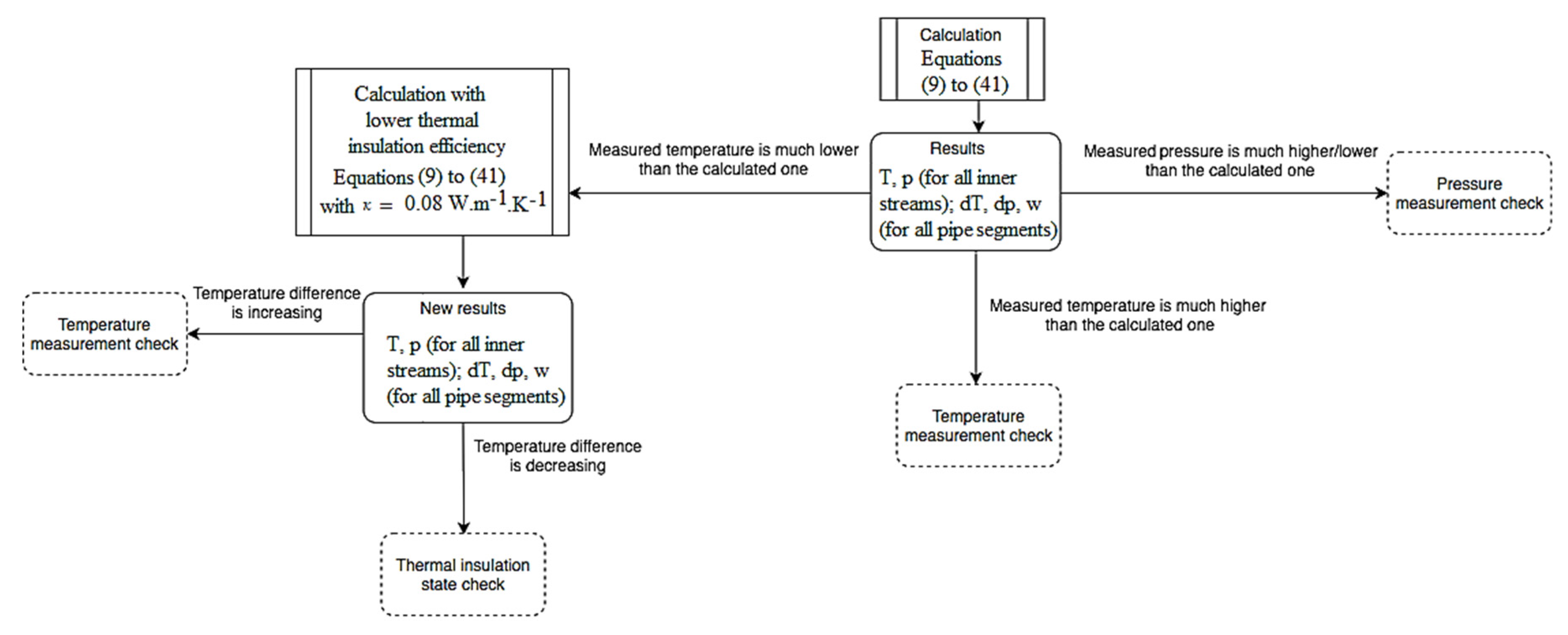
3.3.3. Model Validation (Analysis of Actual Operation)

One of the issues solved was the mass balance difference. The result of the balance model was used as follows: Measured steam flows at each outlet stream were adjusted in the way, the mass balance difference was distributed through all outlet streams proportionally, i.e., based on the ratio of the steam flow to total steam supply. This modification is expressed as follows Equation (41) and ensures an equal distribution of steam balance difference (eventual losses):

$${\dot{\mathrm{m}}}_{\mathrm{f},\mathrm{i}}={\dot{\mathrm{m}}}_{\mathrm{m}\mathrm{e}\mathrm{a}\mathrm{s},\mathrm{i}}+\mathsf{\Delta }{\dot{\mathrm{m}}}_{\mathrm{i}}\frac{{\dot{\mathrm{m}}}_{\mathrm{m}\mathrm{e}\mathrm{a}\mathrm{s},\mathrm{i}}}{{\dot{\mathrm{m}}}_{\mathrm{i}\mathrm{n},\mathrm{t}\mathrm{o}\mathrm{t},\mathrm{i}}}={\dot{\mathrm{m}}}_{\mathrm{m}\mathrm{e}\mathrm{a}\mathrm{s},\mathrm{i}}\left(1+\frac{\mathsf{\Delta }{\dot{\mathrm{m}}}_{\mathrm{i}}}{{\dot{\mathrm{m}}}_{\mathrm{i}\mathrm{n},\mathrm{t}\mathrm{o}\mathrm{t},\mathrm{i}}}\right)$$

(41)

where the subscript f,i relates to the balanced mass flow of the i-th outlet stream and the subscript meas,i means the measured mass flow of the i-th outlet stream. The calculation steps are performed by an algorithm depicted in Figure 2.

In step 0, the initial steam parameters are imported from the real measured data. Thermodynamic properties are determined. For simplification, steam parameters are assumed to be constant throughout individual pipe sections in this step. Step 1 involves mass balance, which is crucial part for next calculations. Subsequently, steam flow velocity in each pipe section can be determined as well in step 2 (Equation (1)). Pressure drop in each section is calculated using combination of Equations (6)–(34). Step 3 involves calculation of heat losses in each pipe section, Equations (35)–(40). This step also includes recalculation of overall heat-transfer coefficient, U_inn, in each iteration. From known values of heat losses, values of the steam temperature decrease can be obtained. This is important for recalculation of steam parameters in step 4.

The objective function of the model is the sum of differences of pressure drops in two following iterations squared. The value of parameter k was determined based on previous experiences to obtain results with sufficient accuracy in acceptable calculation time.

Outputs from the thermo-hydrodynamic model are the following:

• Temperatures of all inner and outlet streams;
• Pressures of all inner and outlet streams;
• Temperature drops in each pipe segment;
• Pressure drops in each pipe segment;
• Steam flow velocities in each pipe segment.

Validation/verification of this model was done by comparison of calculated and measured values of temperature and pressure at the outlet streams. The average relative errors for i-th stream are calculated by Equation (42):

$${\overline{\mathsf{\delta }}}_{\mathrm{a},\mathrm{i}}=\frac{1}{\mathrm{N}}{\displaystyle \sum }_{\mathrm{j}=1}^{\mathrm{N}}\frac{{\mathrm{a}}_{\mathrm{c},\mathrm{i},\mathrm{j}}-{\mathrm{a}}_{\mathrm{m}\mathrm{e}\mathrm{a}\mathrm{s},\mathrm{i},\mathrm{j}}}{{\mathrm{a}}_{\mathrm{m}\mathrm{e}\mathrm{a}\mathrm{s},\mathrm{i},\mathrm{j}}}$$

(42)

where a = T,P; indices c and meas refer to calculated and measured values, respectively, N is yearly working time fund, i.e., count of data sets. Values of relative errors can also help us to identify possibly incorrect measurement tools.

Calculated temperature and pressure drops are directly related to steam flow velocities. Elevated pressure drop indicates high steam flow and on the other hand, elevated temperature drop indicates low steam flow. Calculated steam flow velocities can be compared to those obtained by the balance model and assessed by temperature and pressure losses as well.

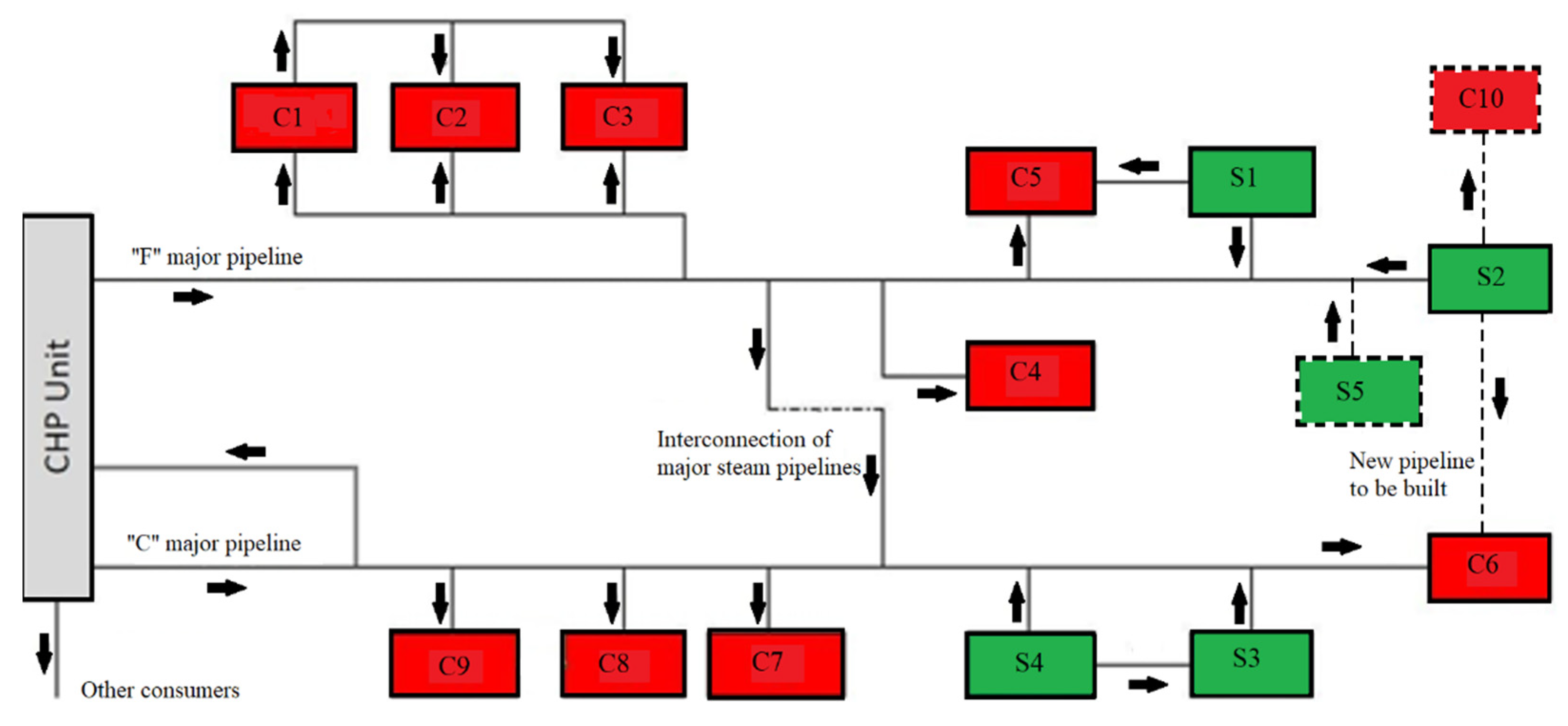
3.3.4. The Impact of Proposed Changes on Steam Network Operation

After model validation (analysis of actual operation), it was used for prediction of transported steam parameters after certain technological changes within the high-pressure steam network. By such simulation it is possible to assess impact of these changes and to identify potential problems. The following changes were considered:

• Direct connection of units C6 and S2 by a new steam pipeline;
• Commissioning of new production unit C10;
• Commissioning new hydrogen production plant S5 thus replacing the old unit S1.

Project A is related only to change of topology, while projects B and C will affect the mass balance of steam networks as well by adding new steam suppliers/consumers. Building a connection between C6 and S2 can change steam flow direction and thus affect steam temperature in adjacent units.

The unit C10 should process part of sour gases from refinery and thus decrease the load of the existing unit sulphur-recovery unit S2 located in its proximity (Figure 3). As a result, the HPS export from S2 will decrease by more than 11 t/h.

New hydrogen production plant S5 is only in the design stage and should substitute the obsolete hydrogen production plant S1 with connection to the HPS network in its proximity (Figure 3). The HPS export should increase from current 11 t/h (from S1) up to 35 t/h (from S5) on average. However, S5 will be able to produce up to 54 t/h steam at its full load, which can be a critical amount due to the transport capacity of the steam pipeline in this section.

Each of these projects will have a significant impact on steam network’s operation. At unchanged loads of other production units, it will be necessary to modify the steam supply from the CHP unit to maintain the steam mass balance. The effect of proposed changes on each steam network is summarized in

Table 5. The effect of proposed changes A, B and C on the steam amount supplied to steam networks. LPS = low-pressure steam, MPD = middle-pressure steam, HPS = high-pressure steam.

Steam Network	Steam Export Change, t/h
	A	B	C
LPS	-	-	−9.2
MPS	-	+7.3	-
HPS	-	−11.6	+25.0

. Simulation scheme of HPS network was modified according to information relating to this project as can be seen in Figure 3.

Data analysis proved that the operation of HPS network varies a lot with season as well as with different loads of other production units. Evidence of this fact is provided in Figure 4 showing a total HPS amount supplied from the CHP unit throughout the year 2017 varying from 0 to 100 t/h. Average ambient temperatures were selected according to local meteorological measurements and they are listed in

Table 6. Selected model parameters and HPS supply into the steam network.

	Date, Time	Ambient Temperature, °C	Wind Speed, m/s	HPS Supply from the CHP Unit, t/h	Total HPS Supply, t/h
Winter	3.1.2017, 10:00	−5	2	53.18	112.3
Spring	22.4.2017, 6:00	10	3	60.93	101.13
Summer	10.7.2017, 19:00	30	3	28.07	97.67

. A representative set of values was selected, corresponding to situations, when ambient temperature was equal to the selected one. Table 6 also contains values of overall HPS supply and HPS supply from the CHP unit at that time.

Simulations were performed with two different values of the thermal conductivity of thermal insulation. The value of κi = 0.038 Wm⁻¹K⁻¹ refers to a new insulation in proper technical state. On the other hand, the value of κi = 0.080 Wm⁻¹K⁻¹ refers to real state of thermal insulation and it was determined based on results of analysis of current operation of steam network and visual inspection in SLOVNAFT, a.s.

4. Results and Discussion

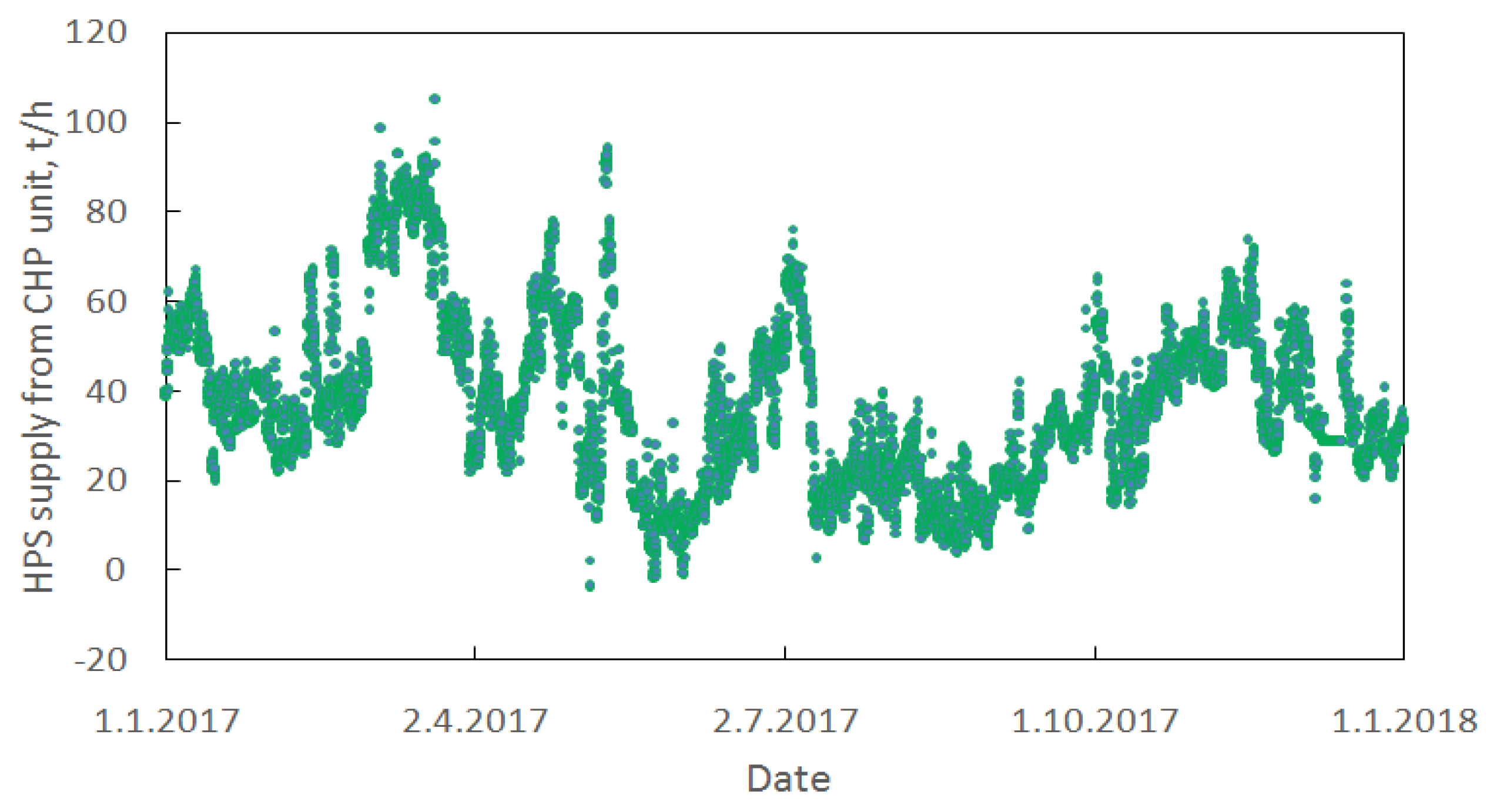
4.1. Data Analysis

The HPS network in the SLOVNAFT refinery is the shortest one with total length of approx. 7 km and there are only 6 steam supplying and 12 steam consuming units connected to it. The share of the amount of HPS supplied from the CHP unit was only 39.52% during year 2017. This means, that this steam network is the least-dependent on the steam supply from the CHP unit. By contrast, the MPS network is the most dependent on the steam supply from the CHP unit with the share of steam amount almost 84% of total one. There is a significant effect of season on steam consumption as well as supply. Figure 5 shows a time-course of LPS supply and the variability of transported steam amounts. Less significant seasonal trends can be observed in the case of the MPS and HPS networks as well. Especially the LPS steam network suffers from exceeding amount of steam supply during summer due to high air temperatures and lower heat utilization. This is common issue in chemical industry, especially in refining and petrochemical industry. In such situations the waste heat-recovery methods should be utilized as much as possible/needed [48]. Moreover, in most critical situations, the exceeding steam is led to the air condenser to decrease its supply into steam network and keep the network balanced.

4.2. Balance Model

The results of the balance model characterize the overall technical state of steam networks in the refinery and the efficiency of their operation. The results of mass and heat balances of each steam pressure level network are listed in

Table 7. Results of mass and heat balances of individual steam pressure level networks.

	$\mathbf{\Delta }{\dot{\mathbf{m}}}_{\mathbf{A}\mathbf{V}\mathbf{G}}$ t/h	${\left(\frac{{\Delta }\dot{\mathbf{m}}}{{\dot{\mathbf{m}}}_{\mathbf{i}\mathbf{n},\mathbf{t}\mathbf{o}\mathbf{t}}}\right)}_{\mathbf{A}\mathbf{V}\mathbf{G}}$	${\left(\frac{\mathbf{\Delta }\dot{\mathbf{m}}}{{\dot{\mathbf{m}}}_{\mathbf{i}\mathbf{n},\mathbf{C}\mathbf{H}\mathbf{P}}}\right)}_{\mathbf{A}\mathbf{V}\mathbf{G}}$	$\mathbf{\Delta }{\dot{\mathbf{Q}}}_{\mathbf{A}\mathbf{V}\mathbf{G}}$ GJ/h	${\left(\frac{\mathbf{\Delta }\dot{\mathbf{Q}}}{{\dot{\mathbf{Q}}}_{\mathbf{i}\mathbf{n},\mathbf{t}\mathbf{o}\mathbf{t}}}\right)}_{\mathbf{A}\mathbf{V}\mathbf{G}}$	${\left(\frac{\mathbf{\Delta }\dot{\mathbf{Q}}}{{\dot{\mathbf{Q}}}_{\mathbf{i}\mathbf{n},\mathbf{C}\mathbf{H}\mathbf{P}}}\right)}_{\mathbf{A}\mathbf{V}{G}}$
LPS	38.13	0.3054	0.5579	104.97	0.2943	0.5323
MPS	21.52	0.2116	0.2770	65,74	0.2294	0.2739
HPS	6.05	0.0646	0.1634	26.57	0.0922	0.2265
Total	44.50	0.1423	0.2401	136.17	0.1463	0.2456

as the average balance difference during the whole year 2017. The balance difference means the difference between the amount of supplied and consumed mass and heat within the steam network, respectively.

Graphical interpretation of mass and heat balance is depicted in Figure 6, Figure 7 and Figure 8.

The average mass balance difference in 2017 in the LPS was 38.13 t/h, i.e., 30.5% of total steam amount supplied from the CHP unit and 55.8% of total steam amount supplied into this network, respectively. This phenomenon could be partially explained due to LPS consumption as steam tracing as well as increased heat losses during the winter months. This consumption is not controlled, and it is very difficult to estimate its amount. There is a significant drop on 15.5.2017, where the steam supply from the CHP dropped by approx. 34 t/h during one single day. However, the total steam measured consumption remained constant. From this reason, the LPS consumption as steam tracing was estimated as high as 34 t/h during the winter months.

Negative LPS mass balance in summer months is seen in Figure 6: when there is no other option to manipulate the LPS steam balance, the LPS is led to air cooled steam condensers. This consumption is not measured which is the explanation of the observed fact.

The mass and heat balance results of MPS network have similar trends as in case of LPS network. Increased balance difference during winter can be explained by increased heat losses to the surroundings and uncontrolled steam tracing. However, the difference between summer and winter is not as sensible as the difference at LPS network. The average mass balance difference is 21.52 t/h. It means the share of 27.70% and 21.16% on the steam supply from the CHP unit and the total steam supply, respectively. The trend of heat balance copies the trend of mass balance. The measurement of temperatures and pressures can be therefore considered as reliable.

The results of HPS mass and steam balance are the most satisfying. The average mass balance difference is only 6.5% of total HPS amount supplied into this network and 16.3% of total HPS amount supplied from the CHP unit, respectively. There are a few drops and peaks, which can be explained by unit shut downs or measurement failures. The biggest drop on 10.12.2017 is highlighted in Figure 8. Input data analysis showed, that during the period from 8.12 to 13.12.2017 all steam flow meters on the CHP unit battery limit showed constant value. The assumption that this is not a failure of the measuring tool, but rather a failure of signal transmission was later confirmed by consultation with energy managers.

Dividing average heat and mass balance difference, the value of theoretical enthalpy of loss of steam, h_t, Equation (43) is obtained. Values of theoretical enthalpy calculated for each steam network compared with typical, h, minimal, h_min and maximal, h_max, values of enthalpy of steam at given pressure level defined by internal regulation are listed in

Table 8. Values of theoretical steam enthalpy and typical values of steam enthalpy in the refinery.

Steam Pressure Level	ht [GJ/t]	h [GJ/t]	hmin [GJ/t]	hmax [GJ/t]
LPS	2.75	2.84	2.76	2.91
MPS	3.05	3.01	2.87	3.09
HPS	4.39	3.07	3.03	3.13

.

$${\mathrm{h}}_{\mathrm{t}}=\frac{\mathsf{\Delta }{\dot{\mathrm{Q}}}_{\mathrm{A}\mathrm{V}\mathrm{G}}}{\mathsf{\Delta }{\dot{\mathrm{m}}}_{\mathrm{A}\mathrm{V}\mathrm{G}}}$$

(43)

Values of theoretical enthalpy of LPS and MPS are inside or close to the interval of typical values defined by internal regulation. Moreover, there is a similar time-course of both mass and heat balances. This shows that temperature and pressure measurements in the LPS network are sufficiently accurate. The value of the theoretical steam enthalpy of HPS is inadequate, since it differs a lot from the typical value of HPS enthalpy. Assuming the enthalpy of 3.1 GJ/t and given mass balance difference, the overall heat losses due to material losses should reach 18.8 GJ/h. The rest of 7.8 GJ/h should be explained by heat loss to surrounding or incorrect measurement of temperature, pressure or both.

The balance model was designed to perform calculations of steam flow velocity in each pipe sections as well, thus aiming to detect the risk of troublesome spots formation within the steam networks. The upper steam flow velocity limit value of 30 m/s was set based on real experience, depicted in Figure 9, as well as in accordance with expert literature [49]. At the moment of highest steam pressure at unit S2 the excess steam was discharged through the pressure relief valve into the environment and the calculated exported steam flow velocity reached value 29.9 m/s as depicted in Figure 9. The following pressure drop resulted from switching a steam-drive into operation, thus reducing the steam amount supplied from the S2 unit into the HPS network.

By contrast, the lower limit value was set as low as 5 m/s based on previous experiences. Results of the balance model show, that there are few problematic sections in each steam network. The most important identified bottlenecks are:

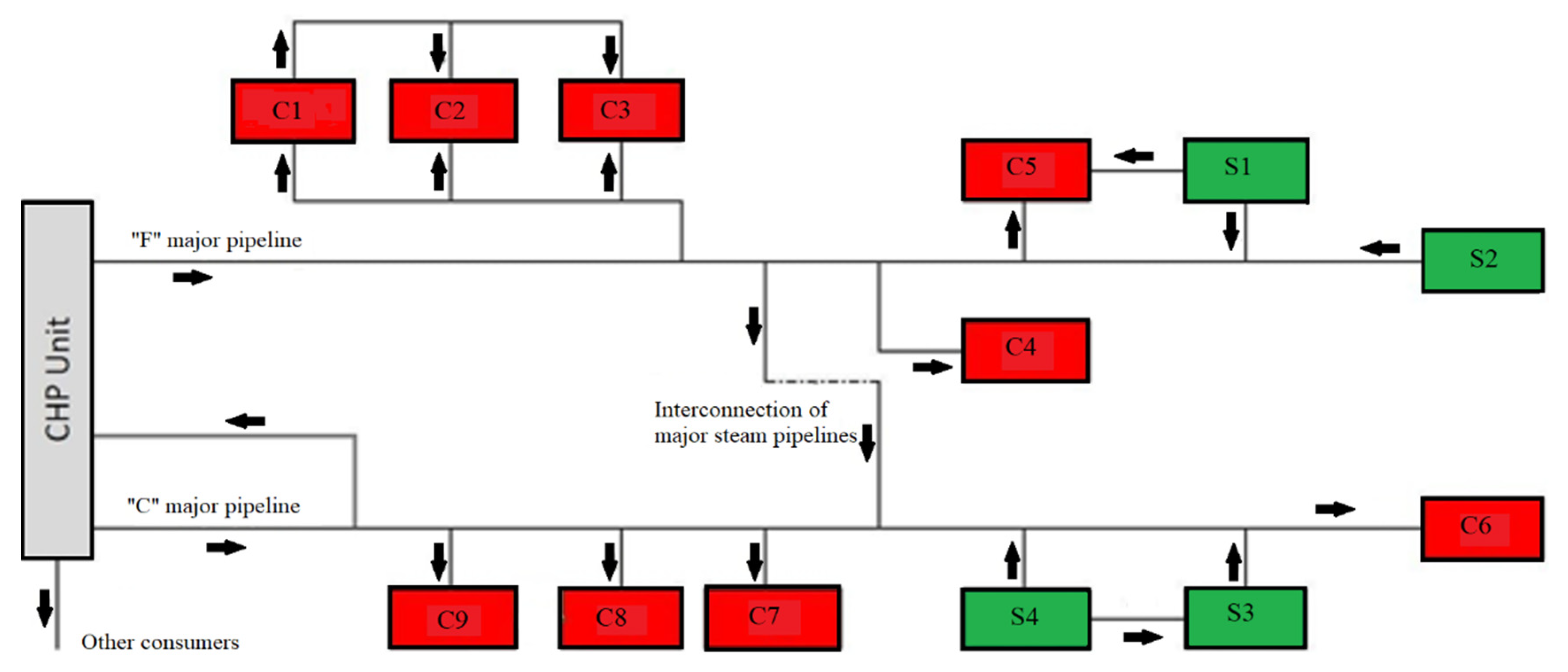
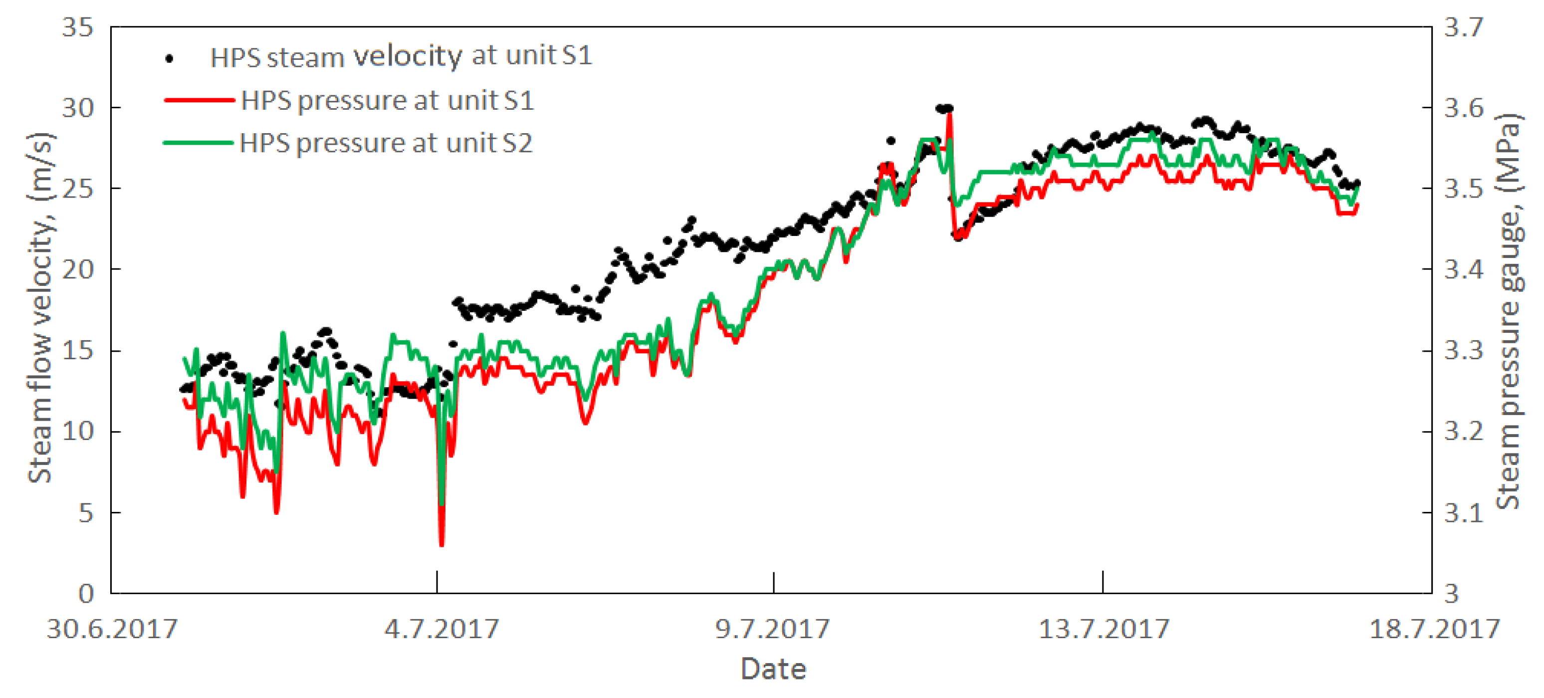
• Section from the C-F main pipeline interconnection to units C5, S1 and S2—this section is problematic due to high amounts of HPS transported as well as due to low steam temperature from S2 unit close to its dew point, which can lead to steam flow velocities over 30 m/s and its condensation.
• The CHP unit export into HPS pipelines E and F. At normal operation, their capacity is sufficient, but can become a bottleneck especially during the winter.
• The CHP unit export into MPS pipeline D—the same reason as indicated in point 2. Moreover, this pipeline supplies the MPS steam to an external consumer and must be able to transport significant amounts of steam in the heating period.

4.3. Thermo-Hydrodynamic Model

Calculated values of steam temperature and pressure were compared to the measured ones and differences as well as relative errors were evaluated. Steam flow velocities were used to determine potential bottlenecks or cold spots. Such identification is possible based on heat loss values as well. High specific heat loss indicates low steam flow rate and vice versa. There is a similar meaning for specific pressure drop. A high value (over 0.3 kPa/m) indicates high steam flow velocity and a possible bottleneck. By contrast, a low pressure drop indicates low steam flow velocity and a possible cold spot.

Results of simulations proved positive as well as negative temperature and pressure differences. The results can be considered reliable with a value of relative error under 5% and values over 10% were excluded and the measurement was marked as “incorrect”. Values of average, minimal and maximal relative errors of temperature and pressure for each network are listed in

Table 9. Average, minimal and maximal relative errors of steam temperature and pressure.

	LPS	MPS	HPS
${\overline{\mathsf{\delta }}}_{\mathrm{T}}/\%$	4.98	2.25	3.21
${\mathsf{\delta }}_{\mathrm{T},\mathrm{m}\mathrm{i}\mathrm{n}}/\%$	1.03	0.35	1.10
${\mathsf{\delta }}_{\mathrm{T},\mathrm{m}\mathrm{a}\mathrm{x}}/\%$	9.51	5.01	9.40
${\overline{\mathsf{\delta }}}_{\mathrm{P}}/\%$	3.54	2.87	3.38
${\mathsf{\delta }}_{\mathrm{P},\mathrm{m}\mathrm{i}\mathrm{n}}/\%$	0.06	0.30	0.20
${\mathsf{\delta }}_{\mathrm{P},\mathrm{m}\mathrm{a}\mathrm{x}}/\%$	9.33	8.52	7.02

. Please note that all values are absolute values, since the difference can be either positive or negative.

According to the results in Table 7, the LPS network is in worst technical state, since the corresponding mass balance difference is the largest here. The impact of this finding on the results shown in Table 9 is the following:

• A large balance difference distributed to all outlet streams could have caused significant relative errors of the thermo-hydrodynamic model.
• The complexity of the LPS network and many interconnections between each pipeline may also have caused large errors.
• Finally, the nominal values of temperature as well as pressure are lowest in the LPS network which means that the same absolute difference yields in higher relative error in LPS network than in the other ones.

4.4. The Impact of Proposed Changes on Steam Network Operation

The purpose of these simulations was to determine, how the proposed changes within steam network would affect the steam network operation and to detect potential operational troubles. The connection of units C6 and S2 (Project A) should solve the problem of comparatively cold HPS delivered to the C6 unit. The temperature at its battery limit is typically within the range 295 to 310 °C. HPS with temperature approx. 300 °C could already be a risk to safety and reliable operation of steam turbines located at this unit based on previous experiences. This is probably the most important parameter observed in these simulations. At present, both mentioned units are located at the ends of main steam pipelines. While unit S2 supplies a significant amount of steam, unit C6 is a less important steam consumer. Moreover, the distance from S2 to C6 is quite long, approx. 350 m. The combination of these two facts leads to low steam flow velocity in this section and accompanied increased heat losses. Connection of units C6 and S2 would mean creating a circuit within the steam network and improving steam flow velocity in this section.

Results stated below refer to winter conditions, as a worst possible scenario for steam network operation. At the period corresponding to the data taken for simulation in winter conditions, the average HPS temperature at C6 unit was reaching 301.9 °C.

Table 10. Temperature of HPS at selected units after changes within the HPS steam network.

Scenario	Steam Temperature, °C
	C6	C5	C4	C7	C8	C9
Present	308.8	300.0	288.6	316.8	311.4	313.7
A	292.9	302.5	291.1	331.1	325.8	328.1
A+B	292.9	305.2	337.4	335.3	329.8	332.2
A+C	293.7	330.4	317.2	315.4	310.4	312.6
A+B+C	295.8	330.4	317.2	315.0	310.1	312.2
B+C	308.8	315.3	303.4	319.9	314.3	316.7

contains results of all simulations. As expected, these projects would affect mostly units adjacent to the place of realization of proposed projects (C6, C5, C4, C7, C8 and C9). Since the change of steam temperature in other units was negligible, they are not listed in Table 10.

The results show, that in case of realization of project A only, the steam temperature at unit C6 will drop by almost 15 °C (assuming unsuitable technical state of thermal insulation). Since the temperature is already low, this decrease would take the steam even closer to its condensation point. Following the results shown in Table 10, one can conclude:

• Only the connection of units C6 and S2 itself will not improve the steam temperature at C6 unit. Continuous operation of this pipeline will not be effective, otherwise a significant temperature drop will be observed leading to unacceptable operation conditions.
• Also commissioning the new unit C10 will not improve the steam quality at C6 unit (case A+B). Although it will lower the load of unit S2, the supplied steam from S2 will flow in the direction of unit C6 anyway.
• The operation of new unit S5 would improve the steam temperature at unit C6 only slightly (case A+C). The reason is the high steam pressure of steam supplied from unit S2 that will make the steam from unit S5 to flow in the opposite direction (from unit S5 to S1 and C5).

Significant steam temperature increase at units C7 to C9 in case A and A+B can be explained by decreased steam supply from unit S2 to pipeline F. This will be compensated by increased steam supply from the CHP unit of high quality with temperature over 360 °C. The calculated pressure drop on the section between units S2 and C6 is 5 kPa, which is comparable to pressure drops in other sections (over the same distance). One can conclude, that, supposing constant steam pressure at other units, the steam flow in this section will be in direction from unit S2 to unit C6 and not in the opposite one. According to these statements, we recommend stopping project A.

Project C will cause a slight temperature decrease at units C7 to C9. Although new unit S5 would supply large amount of steam of relatively high temperature, the temperature will decrease due to heat loss through transport over a long distance from units S5 to units C7, C8 and C9.

Another remarkable observation is that, in summer conditions, the steam supply from the CHP unit would be too low and some action would have to be made. At present, there is a return pipeline “C” that is used to allow the steam flow back to the CHP unit to be consumed there. Another, but less economic, way is to use the steam let-downs or steam drives.

Comparison of presented calculation results with real system operation data cannot be made as none of the examined projects is in proper operation yet. Project C has been postponed by at least three years; project B, though commissioned, did not reach a stable long-term operation yet and project A is on hold.

4.5. Improvement of Steam Network Operation

There is a significant variability of steam consumption during the year and the steam network is designed to handle different amounts of steam under any conditions. The balance model has proven significant imbalance within the steam network. Certain part of this amount is lost as a part of condensate being disposed into the ground. Few spots with leaking steam into the atmosphere were observed during visual inspections as well; however, these losses are not as high as the result corresponding to the balance model.

Despite steam and condensate losses, the most important factor is the inaccuracy of measurement. A simple algorithm, presented in Figure 10 was developed and used to recommend following general measures, concerning routine and preventive maintenance of steam pipelines, along with the best practice in steam system management [49]:

• Regular inspection of steam traps’ operation;
• Regular visual inspection of steam pipelines and isolation;
• Improve the steam condensate recovery system and prevent from its disposal into the ground;
• Regular inspection and calibration of measurement tools.

The inspection of steam traps is done on a regular basis over a period of 2 years. In the last 2 years, more than 13,000 steam traps have been inspected. More than 1000 were out of operation at that time. Of the remainder, 91.2% were working correctly, 7.7% were leaking and only 1.1% were clogged. Steam traps that are not working correctly are replaced by new ones immediately after inspection.

5. Conclusions

The work deals with mathematical modeling as a tool for steam network optimization. The authors developed a simple model based on nodes and pipes and, therefore, it is applicable to any steam network. Simultaneous calculation of matrix Equations allows shortening the calculation time. Model was tested on steam network in SLOVNAFT oil refinery with real process data from the year 2017. Required data consisted mainly of steam flow, temperature and pressure measurements on individual production units, which were used as input data for both models used. The most challenging issue was the lack of certain data, production unit shutdowns and other measurement or data transfer-related issues.

The balance model performs the calculation of steam flow velocity in each pipe, in addition to mass and heat balance. This allowed identification of troublesome spots within the steam network in terms of low (cold spots) or high steam flow velocity (bottlenecks). Results were partly used as input data for the thermo-hydrodynamic model. This model uses exact equations and correlations for pressure drop, heat loss or steam properties calculation. A probabilistic model employing a similar approach as the balance model was recently used to assess and predict the transport capacities, bottlenecks and system operation change after inclusion of new infrastructure in the real gas transmission network in Europe [50].

Comparing the results of simulations to the real measured data, one can conclude that the real state of thermal insulation is bad, since the thermo-hydrodynamic model initially estimated higher temperatures than the measured ones. Subsequently, the simulations were performed again with a higher value of thermal conductivity corresponding to obsolete and damaged thermal insulation of pipes. The results obtained were closer to reality.

A thermo-hydrodynamic model was used to assess the operation of steam networks after implementation of the proposed changes. Simulations of multiple variations were performed with results leading to one conclusion. The connection of units S2 and C6 by a common pipeline does not lead to the desired result. Therefore, it is recommended to abort this action if possible. This model can be used in the future for prediction of future operation states as well. A comparison of model results and real operational data cannot be performed, however, as none of the analysed projects impacting the high-pressure steam network management is in proper operation yet.

The proposed thermo-hydrodynamic model is very complex and sufficiently accurate but requires corresponding skills and knowledge among its users. Moreover, its results are only as reliable as the measurements themselves. During the cooperation with the refinery, a few controlled operation experiments were performed to determine the steam flow in pipe interconnections and to assess the accuracy of individual measurement tools as well. It is recommended to continue with these experiments in the future as well and improve the overall state of steam networks.

References

1. U.S. Department of Energy (DoE), Advanced Manufacturing Office (AMO). Improving Steam System Performance: A Sourcebook for Industry, 2nd ed.; 2012; 64p. Available online: https://www.energy.gov/sites/prod/files/2014/05/f15/steamsourcebook.pdf (accessed on 14 November 2018).
2. Bütün, H.; Kantor, I.; Maréchal, F. Incorporating Location Aspects in Process Integration Methodology. Energies 2019, 12, 3338. [Google Scholar] [CrossRef] [Green Version]
3. Wu, Y.; Wang, R.; Wang, Y.; Feng, X. An area-wide layout design method considering piecewise steam piping and energy loss. Chem. Eng. Res. Des. 2018, 138, 405–417. [Google Scholar] [CrossRef]
4. Nishio, M.; Itoh, J.; Shiroko, K.; Umeda, T. A thermodynamic approach to steam-power system design. Ind. Eng. Chem. Process. Des. Dev. 1980, 19, 306–312. [Google Scholar] [CrossRef]
5. Papoulias, S.A.; Grossmann, I.E. A Structural Optimization Approach in Process Synthesis. Part II: Heat Recovery Networks. Comput. Chem. Eng. 1983, 7, 707–721. [Google Scholar] [CrossRef]
6. Bruno, J.C.; Fernandez, F.; Castells, F.; Grossmann, I.E. A rigorous MINLP model for the optimal synthesis and operation of utility plants. Trans. Inst. Chem. Eng. 1998, 76, 246–258. [Google Scholar] [CrossRef]
7. Varbanov, P.S.; Doyle, S.; Smith, R. Modelling and optimization of utility systems. Chem. Eng. Res. Des. 2004, 82, 561–578. [Google Scholar] [CrossRef]
8. Reddy, C.C.S.; Naidu, S.V.; Rangaiah, G.P. Optimization of a steam network. Chem. Eng. 2013, 52, 54–59. [Google Scholar]
9. Variny, M.; Mierka, O.; Godó, Š.; Illés, P.; Margetíny, T. The Optimization of the High Pressure Steam Consumption and the Steam Pipeline Network Management in the Slovnaft Refinery. In Proceedings of the ICCT 2014, sborník Abstraktů a Plných textů, 2. Mezinárodní Chemicko-Technologická Konference, Mikulov, Czech Republic, 7–9 April 2014; ČSPCH: Praha, Czech Republic, 2014; 6p, ISBN 978-80-86238-61-6. [Google Scholar]
10. Magalhaes, E.G.; Wada, K.; Secchi, A.R. Steam Production Optimization in a Petrochemical Industry. In 4th MERCOSUR Congress on Process Systems Engineering: 2nd MERCOSUR Congress on Chemical Engineering: Proceedings of Enpromer; 2005; 10p, Available online: https://www.lume.ufrgs.br/handle/10183/8315 (accessed on 6 December 2019).
11. Bungener, S.L.; Van Eetvelde, G.; Maréchal, F. Optimal Operations and Resilient Investments in Steam Networks. Front. Energy Res. 2016, 4. [Google Scholar] [CrossRef] [Green Version]
12. Hachicha, A.A. Thermo-hydraulic modelling for direct steam generation. Energy Procedia 2017, 143, 705–712. [Google Scholar] [CrossRef]
13. Price, T.; Majozi, T. Using Process Integration for Steam System Network Optimization with Sustained Boiler Efficiency. In Proceedings of the 19th European Symposium on Computer Aided Process Engineering—ESCAPE 19, Cracow, Poland, 14–17 June 2009; pp. 1281–1287. [Google Scholar]
14. Magalhaes, E.G.; Fronza, T.; Wada, K.; Secchi, A.R. Steam and Power Optimization in a Petrochemical Industry. In Proceedings of the International Symposium on Advanced Control of Chemical Processes ADCHEM 2006, Shenyang, China, 25–27 July 2018; pp. 839–843. [Google Scholar]
15. Bojić, M.; Stojanović, B. MILP Optimization of a CHP energy system. Energy Convers. Manag. 1998, 39, 637–642. [Google Scholar] [CrossRef]
16. Zhu, Q.; Luo, X.; Zhang, B.; Chen, Y.; Mo, S. Mathematical modeling, validation, and operation optimization of an industrial complex steam turbine network-methodology and application. Energy 2016, 97, 191–213. [Google Scholar] [CrossRef]
17. Chen, C.L.; Chen, H.C. A mathematical approach for retrofit and optimization of total site steam distribution networks. Process. Saf. Environ. Prot. 2014, 92, 532–544. [Google Scholar] [CrossRef]
18. Luo, X.; Huang, X.; El-Halwagi, M.M.; Ponce-Ortega, J.M.; Chen, Y. Simultaneous synthesis of utility system and heat exchanger network incorporating steam condensate and boiler feedwater. Energy 2016, 113, 875–893. [Google Scholar] [CrossRef]
19. Zhao, L.; Zhong, W.; Du, W. Data-Driven Robust Optimization for Steam Systems in Ethylene Plants under Uncertainty. Processes 2019, 7, 744. [Google Scholar] [CrossRef] [Green Version]
20. Luo, X.; Yuan, M.; Wang, H.; Jia, Y.; Wu, F. On steam pipe network modeling and flow rate calculation. Procedia Eng. 2012, 29, 1897–1903. [Google Scholar] [CrossRef] [Green Version]
21. Ziping, T.; Fumin, B. Real time simulation in computer for oversize steam networks. J. Shanghai Jiao Tong Univ. 2000, 34, 486–489. [Google Scholar]
22. Chen, Z.; Wang, J. Heat, mass, and work exchange networks. Front. Chem. Sci. Eng. 2012, 6, 484–502. [Google Scholar] [CrossRef]
23. Isafiade, A.J.; Short, M. Synthesis of Renewable Energy Integrated Combined Heat and Mass Exchange Networks. Process. Integr. Optim. Sustain. 2019, 3, 437–453. [Google Scholar] [CrossRef]
24. Xiao, W.; Zhou, R.-J.; Dong, H.-G.; Meng, N.; Lin, C.-Y.; Adi, V.S.K. Simultaneous optimal integration of water utilization and heat exchange networks using holistic mathematical programming. Korean J. Chem. Eng. 2009, 26, 1161–1174. [Google Scholar] [CrossRef]
25. Liu, Q.T.; Zhang, Z.G.; Pan, J.H.; Guo, J.Q. A coupled thermo-hydraulic model for steam flow in pipe networks. J. Hydrodyn. 2009, 21, 861–866. [Google Scholar] [CrossRef]
26. Zhong, W.; Feng, H.; Wang, X.; Wu, D.; Xue, M.; Wang, J. Online hydraulic calculation and operation optimization of industrial steam heating networks considering heat dissipation in pipes. Energy 2015, 87, 566–577. [Google Scholar] [CrossRef]
27. García-Gutiérrez, A.; Hernández, A.F.; Martínez, J.I.; Ceceñas, M.; Ovando, R.; Canchola, I. Hydraulic model and steam flow numerical simulation of the Cerro Prieto geothermal field, Mexico, pipeline network. Appl. Therm. Eng. 2015, 75, 1229–1243. [Google Scholar] [CrossRef]
28. Teixeira, R.G.D.; Secchi, A.R.; Biscaia, E.C., Jr. Two-Phase Flow in Pipes: Numerical Improvements and Qualitative Analysis for a Refining Process. Oil Gas. Sci. Technol. 2015, 70, 497–510. [Google Scholar] [CrossRef] [Green Version]
29. Wang, H.; Meng, H.; Zhu, T. New model for onsite heat loss state estimation of general district heating network with hourly measurements. Energy Convers. Manag. 2018, 157, 71–85. [Google Scholar] [CrossRef]
30. Wang, H.; Wang, H.; Zhu, T.; Deng, W. A novel model for steam transportation considering drainage loss in steam network. Appl. Energy 2017, 188, 178–189. [Google Scholar] [CrossRef]
31. Milosevic, Z.; Ponhöfer, C. Refiner improves steam system with custom simulation/optimization package. Oil Gas. J. 1997, 95, 90–94. [Google Scholar]
32. De, S.; Kaiadi, M.; Fast, M.; Assadi, M. Development of an artificial neural network model for the steam process of a coal biomass cofired combined heat and power (CHP) plant in Sweden. Energy 2007, 32, 2099–2109. [Google Scholar] [CrossRef]
33. Li, Z.; Zhao, L.; Du, W.; Qian, F. Modeling and Optimization of the Steam Turbine Network of an Ethylene Plant. Chin. J. Chem. Eng. 2013, 21, 520–528. [Google Scholar] [CrossRef]
34. Manesh, M.H.K.; Abadi, S.K.; Amidpour, M.; Ghalami, H.; Hamedi, M.H. New emissions targeting strategy for site utility of process industries. Korean J. Chem. Eng. 2013, 30, 796–812. [Google Scholar] [CrossRef]
35. Strušnik, D.; Avsec, J. Artificial neural networking and fuzzy logic exergy controlling model of combined heat and power system in thermal power plant. Energy 2015, 80, 318–330. [Google Scholar] [CrossRef]
36. Dettori, S.; Colla, V.; Salerno, G.; Signorini, A. Steam Turbine models for monitoring purposes. Energy Procedia 2017, 105, 524–529. [Google Scholar] [CrossRef]
37. Beangstrom, S.G.; Majozi, T. Steam system network synthesis with hot liquid reuse: I. The mathematical model for steam level selection. Comput. Chem. Eng. 2016, 85, 210–215. [Google Scholar] [CrossRef]
38. Nemet, A.; Klemeš, J.J.; Varbanov, P.S.; Mantelli, V. Heat Integration retrofit analysis—An oil refinery case study by Retrofit Tracing Grid Diagram. Front. Chem. Sci. Eng. 2015, 9, 163–182. [Google Scholar] [CrossRef]
39. Beangstrom, S.G.; Majozi, T. Steam system network synthesis with hot liquid reuse: II. Incorporating shaft work and optimum steam levels. Comput. Chem. Eng. 2016, 85, 202–209. [Google Scholar] [CrossRef]
40. Majanne, Y. Model predictive pressure control of steam networks. Control. Eng. Practice 2005, 13, 1499–1505. [Google Scholar] [CrossRef]
41. Dzedzemane, R.; le Roux, J.D.; Muller, C.J.; Craig, I.K. Steam Header State-Space Model Development and Validation. IFAC PapersOnLine 2018, 51, 207–212. [Google Scholar] [CrossRef]
42. The International Association for the Properties of Water and Steam. The IAPWS Industrial Formulation 1997 for the Thermodynamic Properties of Water and Steam; IAPWS: Eflangen, Germany, 1997. [Google Scholar]
43. Product Marketing, Aspen Technology, Inc. An. Integrated Approach to Modeling Pipeline Hydraulics in a Gathering and Production System; Aspen Technology, Inc.: Bedford, MA, USA, 2015; Available online: https://www.aspentech.com/en/-/media/aspentech/home/resources/white-papers/pdfs/11-7579-wp_pipeline_hydraulics_d.pdf (accessed on 21 October 2019).
44. Brkić, D.; Praks, P. Unified Friction Formulation from Laminar to Fully Rough Turbulent Flow. Appl. Sci. 2018, 8, 2036. [Google Scholar] [CrossRef] [Green Version]
45. Sutera, S.P.; Skalak, R. The history of Poiseuille’s law. Annu. Rev. Fluid Mech. 1993, 25, 1–20. Available online: https://www.annualreviews.org/doi/10.1146/annurev.fl.25.010193.000245 (accessed on 6 December 2019). [CrossRef]
46. Blasius, H. Grenzschichten in Flüssigkeiten mit kleiner Reibung. Z. Angew. Math. Phys. 1908, 56, 1–37. [Google Scholar]
47. Round, G.F. An explicit approximation for the friction factor—Reynolds number relation for rough and smooth pipes. Can. J. Chem. Eng. 1980, 58, 122–123. [Google Scholar] [CrossRef]
48. Reddy, C.C.S.; Naidu, S.V.; Rangaiah, G.P. Waste heat recovery methods and technologies. Chem. Eng. 2013, 120. Available online: https://www.chemengonline.com/waste-heat-recovery-methods-and-technologies/?printmode=1 (accessed on 5 December 2019).
49. Spirax-Sarco. The Steam and Condensate Loop. Effective Steam Engineering for Today; Spirax-Sarco Limited: Cheltenham, UK, 2011; ISBN 978-0-9550691-5-4. [Google Scholar]
50. Praks, P.; Kopustinskas, V.; Masera, M. Probabilistic modelling of security of supply in gas networks and evaluation of new infrastructure. Reliab. Eng. Syst. Saf. 2015, 144, 254–264. [Google Scholar] [CrossRef]
Figure 1. A part of simplified simulation scheme of high-pressure steam (HPS) network for the balance model (S = steam supplier, C = steam consumer).
Processes 08 00622 g001
Figure 2. Calculation algorithm of the thermo-hydrodynamic model.
Processes 08 00622 g002
Figure 3. A part of simplified simulation scheme of HPS network after implementation of proposed changes (S = steam supplier, C = steam consumer; existing connection of main pipelines = dot-dashed line, new connection of pipelines = dashed line).
Processes 08 00622 g003
Figure 4. The amount of HPS supplied from the combined heat and power (CHP) unit during year 2017.
Processes 08 00622 g004
Figure 5. A time course of LPS steam supply from the CHP unit and its total supply throughout the year 2017.
Processes 08 00622 g005
Figure 6. A difference between the amount of steam supplied and consumed within the LPS network during the year 2017.
Processes 08 00622 g006
Figure 7. A difference between the amount of steam supplied and consumed within the MPS network during the year 2017.
Processes 08 00622 g007
Figure 8. A difference between the amount of steam supplied and consumed within the HPS network during the year 2017.
Processes 08 00622 g008
Figure 9. Time course of HPS flow velocity at S2 unit and HPS pressure at battery limit of units S2 and S1 during the time period from 1.7.2017 to 17.7.2017.
Processes 08 00622 g009
Figure 10. Algorithm used to formulate recommendations for steam system inspections and metering devices check.
Processes 08 00622 g010