1. Introduction
Many industry and research facilities have some of their processes performed under vacuum conditions. Those include semiconductor technology plants, food industry sites and the aerospace industry sites. The existence of vacuum installations induces the need for reliable vacuum pressure monitoring.
A pressure value can provide valuable information about a process and by means of the detection of some gaseous species or leakage, which enables process diagnosis.
Miniaturization goes hand in hand with microfluidics. The designed system contains of a cube crossed by a microchannel where the sensing chip is located. The heat transfer between the chip and its surrounding microchannel allows one to perform the sensing operation.
The miniaturization of sensors relies on microfluidics and allows low cost, low power and non-invasive sensing. In the case of Pirani sensing, the measuring is enabled by device miniaturization. Indeed, the signal to noise ratio is increased by reducing solid thermal conduction.
A vacuum refers to any condition at subatmospheric pressure, which can range from a rough vacuum close to atmospheric pressure to an extremely strong vacuum around 10−10 Pa. Handling such a wide range usually involves several pressure transducers simultaneously integrated inside a chamber. Multiple sensor use in a vacuum chamber raises many issues: integration, maintenance, redundancy, power consumption, wiring and readout to name a few. Extending the sensing range using a single miniature device operating wirelessly is therefore a viable alternative.
The Pirani principle is commonly used to sense pressure in the fine and rough vacuum range. It is based on the heat transfer between a heated sensing element (wire, plate or chip) and its surrounding gas molecules. Since the heat transfer is proportional to the number of molecules, the temperature variation of the sensor depends on the pressure. Heating is necessary to observe a pressure induced temperature variation.
Surface acoustic waves (SAW) propagate on the surfaces of piezoelectric crystals. An interdigital transducer (IDT), which is a set of metallic electrodes etched on the surface of the piezoelectric substrate, converts electrical voltage into waves back and forth. SAW are sensitive to the environment properties like temperature, pressure and humidity. When a material is heated, it is subject to thermal expansion. Its physical properties such as its elasticity, piezoelectricity and permittivity are modified. The variations of those properties are mostly expressed as Taylor series expansions. The resonance frequency of a SAW IDT can be expressed as:
where
V is the wave propagation velocity and
the wavelength which depends on the electrode’s dimensions. At the first order, the sensitivity of the resonance frequency
to the temperature around a reference temperature
is expressed by the coefficient
(in ppm/K):
where
T is the temperature and
is the resonance frequency shift. In [
1], a high-sensitivity wireless temperature SAW sensor is presented. Besides, SAW devices can be easily wirelessly operated [
2].
Several wireless SAW-Pirani sensors are presented in the literature, such as [
3,
4,
5]. In [
6], a GaN membrane SAW sensor that measures simultaneously the pressure and the temperature with the same SAW structure operating as a dual sensor is demonstrated. Sensitivities higher than 60 MHz/MPa for the Lamb mode and about 20 MHz/MPa for the Rayleigh mode were obtained for the structure having fingers and pitches which were 170 nm wide. These values correspond to pressure coefficients of frequency (PCF) of about 3500 ppm/MPa for the Rayleigh and 5400 ppm/MPa for the Lamb mode values, exceeding the values previously reported for SAW pressure sensors. SAW sensors as transducers are shown to be suitable for measuring pressures higher than 1 atm.
In [
7], a SAW pressure sensor is presented. The evaluated sensitivities were 87.81 ppm/K, 900 ppm/MPa and 0.0023 dB/
.
With this in mind, a miniaturised wireless vacuum sensor with extended range and sensitivity was designed, simulated and prototyped [
8,
9]. The assembly of a prototype entailed challenges linked to the operation of two different electromagnetic waves, the miniaturization of all the components and wireless power transfer in a vacuum environment while most components were made of stainless steel. These challenges raised the question of the feasibility of such a solution and its convenience. After manufacturing, assembly issues were addressed and the first characterisation tests were performed.
2. Materials and Methods
The objective of the measurements performed in vacuum was to be able to observe a pressure-dependent signal, i.e., measure a resonance frequency shift vs. pressure through all the vacuum pump pressure range. After characterising the prototype at room temperature and pressure, the prototype was tested and characterised inside a vacuum chamber.
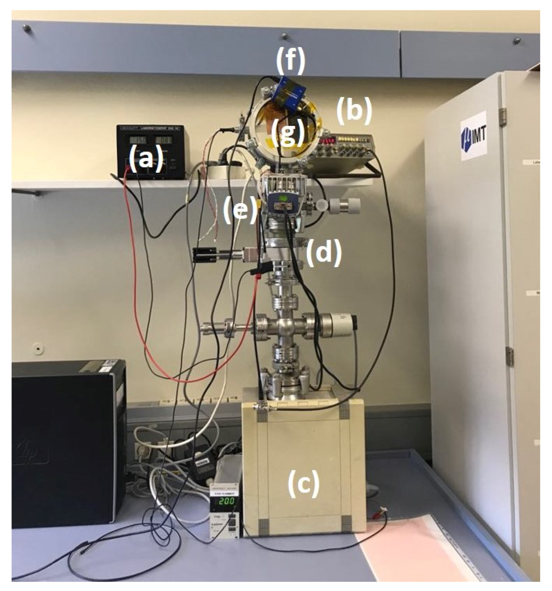
2.1. Description of the Test Rig:
The vacuum test rig shown in
Figure 1 was made of the following components:
Vacuum pump: a TSH071E Turbocube from Pfeiffer Vacuum (Aßlar, Germany) was used to generate subatmospheric pressure conditions.
Metallic ISO KF pipes (METALLIC FLEX, Kirchweg, Germany) were used to connect the components.
A VAT gate valve was used to protect the turbo pump in the rough vacuum region between 10 Pa and atmospheric pressure since it cannot operate under a pressure higher than 10 Pa.
A BCG 450 triple gauge from INFICON (Bad Ragaz, Switzerland) was used as a pressure sensor to monitor the pressure: it contained a Bayard Alpert gauge, a Pirani gauge and a capacitive diaphragm gauge with automatic switch to measure pressures between 5 × 10⁻⁸ Pa and 1.5 × 10⁵ Pa. The pressure sensor contained a display indicating the real time pressure and was connected to a LabVIEW user interface via an RS232 to USB cable.
A needle valve was used to control the pressure.
A window box was prepared to operate the prototype. The sensor was placed inside the box against the window from inside, whereas the interrogation antenna and Tx coil were placed against the window from outside. The PMMA window enabled the propagation of the waves towards and from the vacuum.
In order to test the prototype in vacuum, adjustments to the vacuum chamber were required. It mainly consisted in the preparation of a vacuum PMMA window. Due to the fact that the vacuum viewports available off the shelf are made of borosilicate with a metallisation layer, they are not suitable for SAW interrogation. Companies like VACOM or INFICON commercialise viewports for vacuum optics of several materials and dimensions. The standard viewports are made of borosilicate and fused silicate and show transmission spectra for wavelengths between 0.2 and 5 . The 2.45 GHz SAW wavelength is 1.3836 . The wavelength of the induction wave for coils coupling is in the kilometer range. At first glance the viewport should allow the propagation of the SAW and not the induction wave. However, to prevent tensions occurring during heating, cooling or installing, the viewport contains an intermediate metallisation layer of Kovar (an iron-nickel-cobalt alloy) that prevents electromagnetic waves propagation.
For this reason, a customised polymethyl methacrylate (PMMA) window was manufactured to test the prototype in vacuum. The PMMA circular window had an outer diameter of 160 mm corresponding to the previous viewport diameter and the chamber diameter. The central part of the window, i.e., its 5 cm diameter central circle, had a 2 mm thickness. The transmitting (Tx) coil and Tx antenna were placed outside facing the prototype and the receiving (Rx) coil. Reducing the thickness to 2 mm was done to increase the quality of the signal delivered by the antenna. Since the structure of the chamber did not allow one to put the transmitting coil and the interrogation antenna on different sides, the heating power transfer was separated from the antenna interrogation. The receiver coil was connected to a 10 surface mounted device (SMD) resistor which was soldered on top of the chip.
The prototype inserted inside vacuum consisted mainly of a PCB. On top of the PCB the receiver coil and antenna were mounted. At the bottom of the PCB, the SAW chip was placed. The SMD resistor soldered on top of the SAW chip and connected to the receiver coil was acting as a Joule heating resistance. The soldering of the resistor provided a good thermal contact between the resistor and the SAW chip. A photo of the setup is shown in
Figure 2.
Since the structure of the chamber did not allow placing the transmitting coil and the interrogation antenna at different sides, as could be possible using a smaller ceramic or glass box with an ISO KF or CF junction, the receiver coil was separated from the rest of the PCB. The heating was performed via an SMD resistor to substitute the direct heating of the chip via a gold metallic layer joule resistance at its bottom. The temperature was measured by placing a Pt1000 sensor in the vicinity of the chip inside the vacuum.
2.2. Experimental Procedure
The objective of the test rig was to measure the resonance frequency of the SAW chip versus pressure. After the assembly of the test rig the vacuum pump was turned on. When the ultimate pressure was reached, the pressure was gradually increased by turning the needle valve. The corresponding resonance frequency of the chip was recorded.
Figure 3 shows the complete setup.
The pressure was varied between 0.9 and 100,000 Pa and the behaviour of the chip was observed during one hour by means of a vector network analyser (VNA). Each pressure was maintained over the course of one hour and VNA interrogations were performed every 5 min in order to obtain 10 measurement points for each pressure. Two points per pressure decade were measured. For each pressure value, the measurements were performed when the pressure was stabilised, i.e., 5 min after turning the needle valve to modify the pressure.
The stabilisation of the SAW peak frequency was tracked. The SAW peak was identified from the reflection coefficient
vs. frequency curve via a gain local minimum and a phase local maximum. The MOSFET of the heating unit Tx circuit outside the chamber was supplied with a 16 V square wave at 157 kHz and 0.84 A. The measured output at the receiver coil and heating resistor was 700 mV RMS and 2 V peak to peak. The power provided to the heating resistance was calculated from the voltage measured, which equals:
2.3. Calibration
Prior to the chip interrogation, the network analyser had to be calibrated. Through the use of scattering parameters, the device under test (DUT), i.e., the SAW chip, could be characterised by determining its resonance frequency. At high frequency, scatter parameters are directly related to gain, return loss and reflection coefficient. A VNA’s performance depends on the accuracy of its measurements, which require a preliminary calibration. The calibration process aims to perform a vector error correction to remove errors from actual measurements. An analogy to a VNA calibration process is the zeroing out of a test-lead resistance from an ohmmeter to remove the offset caused by the lead resistance.
The error model of a VNA includes multiple terms for every frequency at which measurements are made. The frequencies where the calibration measurements are made must be carefully chosen in coordination with the frequency range where the VNA is to be used. The calibration process determines the error terms, requires a VNA, cables, and standard probes with known impedance. The calibration is performed by sequentially making measurements using calibration standards. Reliable and suitable connectors and cables handled with care are critical components of the calibration setup. No stresses exceeding their specifications should be applied on them. These calibration standards are one-port and two-port networks that have known characteristics. The one port network is used for reflection mode and the two port network is used for transmission mode. The characterisation of the SAW chip needed only the reflection coefficient , hence a reflection mode with one port network. For this purpose, a three steps calibration standard using a coaxial cable was applied. The three steps are:
Short (S): A coaxial short has a total reflection of magnitude 1. The reflection coefficient of the short is dependent only on its length offset, which represents the length between the reference plane and the short. The loss occurring over this length can generally be ignored. Modelling the short in a VNA requires that only its electrical length be entered into the instrument, but in some cases the model can be extended using the polynomial coefficients to account for parasitic inductance.
Open (O): A coaxial open standard is constructed using a closed design to avoid effects caused by entry of stray electromagnetic energy. At the open end of the inner conductor, a frequency-dependent fringing capacitance is formed. Even if an open standard could physically be constructed with a length of 0, fringing capacitances would result in a negative imaginary part for at higher frequencies.
Match (M): A match is a precision broadband of 50 impedance that has a value corresponding to the system impedance.
The open-short-match technique described above is the most popular for one-port calibration. It uses the three standards connected one after the other to the test port and the relations occurring for wave-quantities a1 to b1 are determined. The behaviour of the individual standards is assumed to be known. The corresponding descriptive models are stored in the vector network analyser. Based on the three derived values, the three unknown quantities (source match, directivity, and reflection tracking) can be calculated.
The three calibration probes were included with the VNA. A calibration was performed for every new set of measurements (position changing, modification of the test rig). The SAW peak frequency was always situated between 2.4 and 2.5 GHz. The frequency sweep was performed first between 2 and 3 GHz and then between 2.4 and 2.5 GHz. The calibration was adjusted accordingly; i.e., the number of calibration points was increased from 1000 to 30,000 between 2 and 3 GHz in the calibration file of the VNA. Frequency steps of 1 kHz were generated. A smoothing algorithm was applied to all the measurement points. A smoothing algorithm is an averaging function that works over a single sweep. The percentage, or aperture, is adjustable up to a maximum of approximately 20–25% of the span (depending on the specific network analyser). The result is a smoothing of the trace by the vector network analyser and the outcome is similar to video bandwidth filtering in a spectrum analyser. The smoothing reduces the noise and increases the signal to noise ratio (SNR).
For each frequency point and its associated window the algorithm normally looks for the mid-point using adjacent data. However, at the beginning and end points (of the measurement span), the algorithm performs a look ahead and look behind. This provides the smoothing function the same number of points for the smoothing window at the beginning and end of the sweep. For noise reduction, averaging is more appropriate, allowing noise to be averaged out. The main disadvantage is that increased averaging factors increase the required measurement time. For averaging, VNAs use sweep-to-sweep averaging in which each data point is computed based on an exponential average of consecutive sweeps weighted by a user-specified averaging factor. Each new sweep is averaged into the trace until the total number of sweeps is equal to the averaging factor for a fully averaged trace. Each point on the trace is the vector sum of the current trace data and the data from the previous sweep. A high averaging factor gives the best signal-to-noise ratio but slows the trace update time. Averaging applies to each s-parameter per measurement channel, no matter which s-parameters are actually displayed. Regardless of the sweep type, the results of the averaged/corrected trace were placed in the analyser’s internal data arrays.
3. Results
The first characterisation of the prototype in vacuum aimed to evidence a pressure-dependent behaviour. This setup allowed to obtain wirelessly a pressure-dependent measurement signal via the use of a miniaturised coil and antenna in vacuum and validates the sensor feasibility and concept of miniaturised wireless vacuum sensor.
Different windows were tested. The standard viewport from INFICON made of borosilicate with a metallisation layer and 10 mm thickness did not grant any SAW signal. The rest of the measurements were performed using the custom made PMMA window described in the materials and methods section. The operating frequency chosen for the heating unit, 157 kHz, is the one that gave maximum output voltage at the heating resistor. The voltage output at the receiver coil that is directly provided to the 5
heating resistance equals to 0.7 V RMS, which corresponds to 100 mW of power approximately. The simulated chip needs 24 mW. The requirements of the heating unit were fulfilled. No SAW peak frequency shift was observed if there was no heating. The observed response time was 1 min approximately. The SAW peak frequency was stabilised one minute after the pressure was modified. The response times calculated (100 s) are therefore realistic. At some pressures, two SAW peaks instead of one were observed in a repeatable way. The behaviour of the antenna signal itself depends on the vacuum pressure. At some pressures the antenna also shows two resonance peaks instead of only one, as shown in
Figure 4. The second peak may correspond to a harmonic of the main resonance frequency or some reflection phenomenon.
From
Figure 4, it can be seen that the operation of the pump influences the signal of the antenna. A secondary self resonance of the antenna can be seen left from the SAW peak. The SAW peak is located between 2 antenna self resonances. A rule of thumb criterion to identify a resonance is an
value below −15 dB. In the upper graph (a) only the second self resonance of the antenna approaches this value, the SAW peak and the first antenna self resonance approaches −10 dB.
A pressure-dependent signal was obtained. When the pressure increases the temperature of the chip decreases. When the temperature decreases the resonance frequency increases. When the pressure increases the resonance frequency increases as well. The criteria to identify the SAW peak frequency were a local minimum of the gain and a local maximum of the phase. The sensitivity is higher between 0.1 and 1 kPa than close to atmospheric pressure. The results obtained with the prototype are shown in
Figure 5.
The sensitivity
of the sensor to pressure is defined as:
where
is the resonance frequency of the chip; P the pressure and T the temperature; the pressure coefficient of frequency PCF is:
where
is the resonance frequency of the chip, P the pressure and T the temperature. The sensors shows a linear behaviour.
The temperature sensitivity
is defined as:
where
is the resonance frequency of the chip and T the temperature.
The temperature coefficient of frequency TCF is defined as:
where
is the resonance frequency of the chip and T the temperature. If the frequency shift vs. pressure and temperature is linear, the resonance frequency can be expressed as:
where
is the resonance frequency at the temperature
and the pressure
;
is the temperature sensitivity; and
is the pressure sensitivity.
The sensitivity in Hz/Pa changes for the different pressure ranges and is reported in
Table 1. The average sensitivity is 5880 Hz/Pa, i.e., 2.4 ppm/Pa between 0.9 Pa and atmospheric pressure. Inside the vacuum, the resonance frequency of the SAW chip measured changed with respect to pressure. The resonance frequency increased with the pressure between 244,7989,448 Hz at 0.871853 Pa and 2,448,780,148 Hz at 99,722.23 Pa. The sensitivity constantly decreased with the pressure according to the expectations between approximately 42 kHz/Pa at 0.9 Pa and 1 Hz/Pa at atmospheric pressure. The sensitivity is higher in the rough vacuum area between the minimum pressure and 200 Pa approximately corresponding to the limit between the Knudsen regime and the transition regime [
8], which corresponds of Knudsen number close to 1 [
10]. The Knudsen regime is not explained in detail here but in [
11]. The uncertainty of the pressure sensor used as a reference is 15% and the uncertainty of the frequency was taken as a first approximation as the double of the standard deviation of the measurements. Since those measurements constitute only a proof of concept, no extended uncertainty analysis was performed. The objective was to observe the rough signal measured in vacuum and determine if the behaviour of the chip is influenced by the value of the vacuum pressure.
Table 1 and
Figure 6 show the computed sensitivity of the sensor.
The values of the gain at SAW peak frequency are similar and do not really depend on the pressure level. The mean value of the gain at the SAW peak frequency is −3.85 dB and the standard deviation is 0.18.
Figure 7 shows the values of the gain of the SAW peak versus pressure.
The values of the gain at the SAW peak frequency are shown in the graph between −4.03776 dB at 2058.71 Pa and −3.417872525 dB at 99,722.23157 Pa. No real trend could be observed despite a continuous increase of pressure. The standard deviation of the gain is stable for each value of the pressure around 0.15%.
The value of the phase at the SAW peak frequency shown in
Figure 8 also does not show any obvious trend, have values between 15¼ and 25¼ with a mean value of 23.53¼ and a standard deviation of 3.05¼. The values of the phase at peak frequency are situated between 15.87451 at 99,722.23 Pa and 26.36852 at 69,677.32 Pa. The standard deviation of the pressure reported in
Table 2 increases with the pressure level, which consolidates the statement of the manufacturer that the uncertainty of the sensor represents 15% of the value of the measurement. The standard deviation of the pressure is always lower than 2% which is much beneath the uncertainty claimed by the manufacturer of the measurement value in any case. The sensitivity decreases when the temperature increases.
4. Discussion
4.1. Sensitivity
The sensitive device is made of lithium niobate Y + 41
− X and has dimensions of 3 mm × 3 mm × 1 mm, which corresponds to the SMD 3 × 3 mm packaging. The SAW wave generated has a temperature coefficient of frequency (TCF) of 19 ppm/K. The equilibrium temperature is 65
for a pressure of 0.9 Pa. The heating capacity is 49 mW.
Figure 9 shows the equilibrium chip temperature corresponding to each pressure value.
Three regimes can be distinguished in the output curve:
The Knudsen regime from 0.9 Pa up to 200 Pa approximately, where the highest sensitivity is reached.
The transition regime from 200 Pa up to 7000 Pa approximately where the sensitivity takes intermediate values.
The convection regime approaching atmospheric pressure where the sensitivity is even lower than in transition regime in the range of 1 Hz/Pa.
The sensitivity rapidly decreases when the pressure increases. This was expected. It is due to the exit of the Knudsen regime as pressure increases and the corresponding evolution of the gas thermal conductivity towards a constant asymptotic value. The mean free path of the gas molecules at ambient temperature decreases very quickly between 0.01 and 100 Pa from 0.1144 m to 0.0011444 m which corresponds to a Knudsen number from 0.715 to 7.15. Considering the dimensions of the chamber whose diameter is 0.160 m, the pressure range tested corresponds to the transition from the Knudsen regime to a regime with a constant thermal conductivity hence the observed responses. The experimental curve of the sensitivity versus pressure is shown in
Figure 6. It was obtained by deriving the values of resonance frequency with respect to pressure. The equilibrium temperature of the chip for each pressure is shown in
Figure 9. The equilibrium temperature was computed from the value of the resonance frequency using the temperature coefficient of frequency provided in the technical sheet of the chip which is 18.857 ppm/K.
The response of the sensor to the pressure is non linear. First of all the Pirani sensing curve has a characteristic S-shape [
8] due to the nonlinear relationship between the gas thermal conductivity and pressure. However, eliminating thermal losses, eliminating the offset of the signal and applying a proper algorithm to the output signal may significantly increase the sensor linearity.
The experimental points obtained are compatible with the theoretical expectations in their trend. This means that the SAW peak frequency increases when the pressure increases with a higher sensitivity in the fine vacuum region between 0.1 and 1000 Pa than between 1000 and 100,000 Pa in the rough vacuum area. This was to be expected from the Knudsen regime analysis, since the thermal conductivity tends towards a constant value approaching atmospheric pressure.
Another less impactfull phenomenon can explain the decrease of sensitivity when the pressure increases. The sensitive device cools down when the pressure increases. The sensitivity of the device to the pressure decreases when its temperature approaches the ambient temperature. This phenomenon is nonetheless less influential than the exit of the Knudsen regime.
4.2. Uncertainty
Every measurement is subject to measurement uncertainty, which is the statistical deviation of the measured values from their true value. There are two types of measurement uncertainty: random uncertainty and systematic uncertainty. Random uncertainties vary with time and are thus unpredictable. While they can be described by statistical analysis, they cannot be removed by calibration. Common random uncertainties include those related to instrument noise and the repeatability of switches, cables, and connectors. On the contrary, systematic uncertainties occur in a reproducible way. They are caused by imperfections in the VNA and can be taken into account by means of calibration.
The severity of the random uncertainty can be mitigated by adopting careful and meticulous measurement practices, such as allowing the instrument to achieve thermal equilibrium, using high-quality cables and connectors, selecting a small frequency bandwidth, and using averaging. This was attempted by working in a temperature controlled environment, using thick cables less vulnerable to bending, working on a restricted frequency range corresponding to the location of the SAW signal and using averaging algorithms. A VNA is also sensitive to its surrounding temperature, which can cause a drift. This was addressed by working in a temperature controlled lab with 1 drift.
An uncertainty analysis and a statistical analysis were performed. The error bars were computed based on the standard deviation (shown in
Table 2). The sample mean value and standard deviation were computed.
This uncertainty remains acceptable given the uncertainties on each system parameter (pressure, TCF, and heating power). The agreement between the theoretical curve and the experimental response is within a range of +/−20%. This allows one to validate the dynamic model of the SAW-Pirani developed. Variations of 1 Pa can be clearly detected. A zoom on the noisiest SAW peak makes it possible to estimate the limit step of measurement at about 1.5 kHz.
The experimental points are compatible with the theoretical expectations. The similarity between theory and experimental results validates the theoretical model to compute the sensitivity of a SAW-Pirani sensor. The precision of the reference sensor is not constant and depends on the pressure range. The sensitivity decreases continuously through the pressure range. The uncertainty of the gauge is 15,000 Pa close to atmospheric pressure and 1.5 × 10⁻⁵ Pa in a strong vacuum. This diminution also accounts for the discrepancy observed between the experimental results and the theoretical curve computed for a gas in the Knudsen regime. The theoretical curve corresponds to the maximum sensitivity. It was therefore expected that experimental results would be of a lower quality. There are also other sources of uncertainty among which the equilibrium temperature that depends on the pressure, the ambient temperature and the input voltage fluctuations.
No frequency counter was used since there was more interest in the shift than in the actual value itself. The basis frequency depends on the thermal resistance and the size of the device.
However, no extended uncertainty analysis was carried on. The analysed system is a prototype, many practical aspects were validated and a qualitative result was expected: the trend of the resonance frequency versus pressure. Extensive uncertainty analysis should be performed only after optimisation of the prototype and optimised integration inside vacuum.
4.3. Signal Processing
In the Pirani sensing the thermal losses are conduction losses and then gaseous thermal transfer losses. Since the gaseous heat transfer is faster, the response time decreases. When AC current is applied, the response time generates a phase between the input signal and the temperature rise. It is easy to observe by performing a frequency sweep to the nanowire. When the pressure in the chamber is modified, the time constant is modified and the temperature response is shifted. The quasi-static approach is no longer valid. The nanowire and the gas gap are considered as thermal resistances and capacitances in parallel and subject to heat flux. When the nanowire is transferred from vacuum to gas medium, the thermal resistance decreases which lowers the response time.
A method to reduce noise is to reduce the VNA’s intermediate frequency (IF) bandwidth. The IF bandwidth is a digitally implemented variable filter used to reduce noise. Narrower IF BW’s result in additional data samples at each frequency point sample. The effect is similar to averaging. However, IF bandwidth reduction results in an increase in point-to-point averaging. Normal averaging, as noted earlier, is a sweep-by-sweep or trace-by-trace average. The minimum measurable frequency step is 1 kHz, this is the sensitivity of the network analyser. Measurement performance depends on the calibration standard chosen, and on the repeatability of the measurement system itself.
A visual criterion was used to identify the SAW peak, an algorithm is needed with clear conditions to identify the SAW peak. These points can be compared to the curve obtained with the simulation of 100 ppm/K calculated with a surface emissivity of 0.75. The experimental values follow the expected trend but are quite far from the orders of magnitude expected.
4.4. Comparison to Other Works
In [
10], to determine the sensitivity of the device close to the Knudsen regime, the ultimate pressure of the pump was maintained during the whole experiment. The power injected in the heating resistor was increased by threshold. For each threshold, after the thermal equilibrium was reached and the temperature computed, the pressure was variated by a few tenths of Pa. The relative frequency shift generated by this threshold was measured and the ultimate pressure reinstalled. The sensitivities of the device for each threshold were extracted.
In [
12], several low pressure gauges are compared. An uncertainty analysis is presented. The most important source of noise identified was the short term random noise. The short term random noise creates instabilities in zero-pressure readings. Another source of uncertainty is, for heated gauges, thermal transpiration at absolute pressures below 100 Pa. At higher pressures performance is limited by long-term shifts in calibration with time (months to years). Random noise limits the smallest pressure change that can be resolved by a transducer. A measure of the noise-limited pressure resolution is given by twice the standard deviation of repeated readings at a stable pressure. The resolution of different transducers tends to scale linearly with their full scale range. The capacitive diaphragm gauges (CDGs) have a resolution of about 1 part in 106 of full scale (FS) range, quartz based transducers about 1 part in 106 to 3 parts in 106 of FS and MEMS-type transducers at about 4 parts in 106 to 10 parts in 106 of FS. As of their availability with lower FS ranges, CDGs have the best absolute pressure resolution among the transducers. The zero instabilities in transducers manifest themselves primarily in two ways. They appear either as zero shifts that correlate directly with changes in room temperature, or as zero drifts that vary randomly in both sign and magnitude and are probably due to drifts in electronics and/or mechanical structure of the gauge.
In [
13], a stable resonant pressure sensor fabricated using 3-D micromachining process is described. Two resonators are located on the surface of a diaphragm and applied pressure is measured from the difference of two resonant frequencies. The sensors is located in a 6.8 × 6.8-mm wide, 0.5-mm thick silicon chip. The resonator has a high Q-value of 50,000. The principle of a resonant pressure sensor is easily understood by an analogy of the phenomenon in which a natural frequency of a string changes due to tensile force. EPROM in the pressure receiver stores the sensor parameters for signal linearization and wide range temperature compensation.
A PhD thesis by Ruellan [
14] presents many interesting conclusions. Ruellan proposes to use the transient regime to reduce response time of thermal conductivity pressure gauges. Using AC signal increases the sensitivity by reducing the noise. Reducing the noise also comes with a reduction of drifts. This can be seen by applying pressure thresholds to the sensing device. The omega method is used to determine thermal conductivity. The small response time can be measured by applying a step current to a nanowire and observing the voltage output. A simple nanowire has a resistance in the range of
. The capacitance of a coaxial cable is in the range of 100 pF. For a 1 m cable of 20
, the characterstic response time is 2
. This time is close to the thermal response time of the device. The electric filtering may disturb the measurement. A solution to this can be the use of parallel nanowires to reduce the overall resistance. Coaxial cables tend to be replaced by twisted pairs that have a lower lineal capacitance. Short pairs are preferred to reduce the capacitance to the maximum. The cabling used for signal acquisition impacts the response time in the
range. The response time depends on pressure.
4.5. Outlook
Considering all the limitations and adjustments currently required, it can be asked whether the designed sensor and prototype represents an advantageous solution for the future.
The commercially available viewports do not allow the transmission of either waves. Besides, to prevent tensions occurring during heating, cooling or installing, the viewports contain an intermediate metallization layer of kovar (an iron-nickel-cobalt alloy) that prevents electromagnetic waves propagation. PMMA is not the best material to use in vacuum due to its poor mechanical stability. When vacuum was applied it was systematically bending which presented a risk of failure for such a small thickness. Viewports of ceramics without metallization or quartz should be considered for further tests. In [
10] a fused quartz window is used to perform transvacuum measurements. Other distances due to the interrogation antenna and PCB were introduced. The reference [
15] highlights the wireless charging procedure of a metallic device. It addresses the issue of electromagnetic waves transmission in metals. In vacuum most equipment is in stainless steel or aluminum, using the surrounding metals as an intermediate coil for induction coupling could be a solution. If this method can also be transposed to antenna operation, there will be no need for windows anymore.
The sensitivity and repeatability of the measurements were assessed. The presettings of the VNA software influences the quality of the measurement signal without modifying the hardware structure. A VNA of better signal quality and denser frequency sweep should be used to obtain a better precision. Since the prototype tested is not a final product, there is no use of an extended calibration according to international standards yet. For this purpose, a pressure calibrator (AMETEK JOFRA AP010C, AMETEK, Inc., Berwyn, PA, USA) [
16] could be used.
The final setup in vacuum aimed to operate the prototype wirelessly and see its response. The position of each of the components strongly influences the measurement signal. All the components impact the measurements. In [
17], an ultrasonic interferometer is presented. Factors for accurate low pressure manometry include the control of thermal and mechanical instabilities.
The sensor itself shall have higher performances thanks to successful manufacturing processes. In order to enhance the performances of the prototype, many improvements in the manufacturing should be made. The SAW device should directly be suspended by wires to the substrate to eliminate the solid conduction heat losses. The heating resistance should be etched around the IDT directly in contact with the gas during the lithography process prior to the dicing.
The PCB containing the heating and interrogation unit should also be adapted to support the suspended chip by containing a hollow at its center aligned to the position of the microchannel. The SAW chip of the sensor is made of lithium niobate Y + 41-X. However, using the YZ cut of the same lithium niobate crystal increases the temperature sensitivity up to 100 ppm/K which increases the temperature sensitivity by approximately five times. The results presented so far can be compared to the theoretical sensitivity curve mentioned above. For this purpose the experimental sensitivities should be multiplied by a correction factor to take the TCF difference into account. This factor equals to 100/19 = 5.3 approximately. In order to improve the SAW Pirani performances, a more robust and easier to manufacture prototype should be produced. The IDTs can be in Ti/Au or in Ta/Pt. The Ti/Au electrodes can be used at low temperature. A diffusion phenomenon followed by the oxydation of titanium in gold at higher temperature forbids their use beyond 300 . The Ta/Pt structure is not subject to this issue and can be operated at very high temperatures. The use of a Pt heating resistor enables the direct measurement of the substrate temperature with conventional Pt 100 gauge for instance.
A dynamic model needs to be validated now to forecast the response time of the sensor with respect to its geometry and its thermal resistance. It might then be possible to detect 0.0001 Pa. Finally, the sensitivity can be increased and the limit step further reduced by metallizing the surface of the sensing element. The experimental results also confirm the theoretically planned measurement range.
Figure 5 shows the response of the SAW-Pirani over a wide range of pressure values, without forced convection device. Further experiments would have to show whether it is possible to remove the zero sensitivity area (regime 2) by means of a forced convection device.
5. Conclusions
A prototype of a compact wireless SAW Pirani vacuum sensor was manufactured and tested. Measurements inside vacuum betwwen 0.9 Pa and atmospheric pressure allowed to test the complete prototype inside vacuum with its components—the sensing chip, the heating unit, the interrogation unit, the PCB and the packaging. Completely wireless measurements were performed via induction coupling and antenna reflection in order to observe a pressure-dependent behaviour of the chip.
There is still room for improvement in almost every aspect, mainly the vacuum interface, the electrical contacting of the chip and the antenna coupling. However, the technical solution imagined to wirelessly measure vacuum pressure with a compact sensor proved to be feasible.

 ,
, 


