1. Introduction
Industry 4.0 is taking its course and continuously raising new challenges to classical process operation and management functions. One pillar of any production system is related to guaranteeing the stability, consistency and predictability ofF industrial processes. This was and it will always be a major concern for industry. Juran considered it as a fundamental function for implementing any quality management systems (the Juran trilogy of Planning, Control and Improvement), and it is an intrinsic part of every Quality standard, deeply embedded in the celebrated ISO 9000 series. Traditionally, this function is operationalized in the shop floor using variation management and reduction methodologies such as Statistical Process Monitoring (SPM), Engineering Process Control (EPC), or combined versions of them [
1,
2,
3,
4], as well as other approaches like error-proof systems (Poka Yoke). However, the way SPM is implemented in industry is changing, as a result of, among other possible drivers: (i) increasing complexity of the processes/products under monitoring and (ii) the new challenges imposed by data collected from them.
Regarding the first category of drivers, current processes under monitoring can present characteristics (almost) absent from the scenarios where, during over 80 years, most SPM technology was developed, such as: they can present stationary dynamics (autocorrelation) [
5,
6,
7,
8,
9,
10] or non-stationary dynamics (such as discontinuous or batch processes) [
11,
12,
13,
14]; multiple set-points and operations modes [
15,
16,
17]; processes have a complex network structure and are composed of many sub-process in series or parallel [
18,
19,
20,
21,
22]; processes are intrinsically multiscale in space and time [
23,
24,
25,
26,
27].
The second category of drivers are connected to the new data-intensive environments industry is currently immersed in. SPM is a data-driven methodology, as its implementation strongly relies on the analysis of historical data (Phase 1 analysis) and data collected during operation (Phase 2 analysis) [
28]. The vast majority of SPM methods were developed to handle scalar (0
th order tensor) sensor like data, either univariately [
29,
30,
31] or multivariately [
32,
33,
34,
35]. More recently, profile monitoring emerged as a new SPM branch dedicated to functional relationships [
36,
37,
38] or higher-order tensorial data structures such as: near-infrared (NIR) spectra [
39,
40,
41], surface profilometry [
37], grey-level images [
42], colour and hyperspectral images [
43,
44,
45,
46,
47], hyphenated instruments [
48] among others, expanding the SPM domain to new processes/products.
The one aspect shared by all methods proposed in the past and the fundamental premise established since the seminal work of Walter A. Shewhart [
31], is that all common cause variation must be present in the reference historical Normal Operating Conditions (NOC) dataset collected to conduct Phase 1 analysis, i.e., in order to assess process stability and establish the control limits for the monitoring statistics. However, this fundamental premise does not hold in many processes, such as the assembling processes in the microelectronics industry using Surface Mount Technology (SMT), which is the focus of our paper.
To make our presentation more objective and clearer, in the following sub-sections we will describe our problem and provide and introductory sketch of the proposed solution.
1.1. Problem Statement: Process Monitoring of Surface Mount Technology (SMT) Production Lines
The assembly process of complex electronic devices involves placing, fixing and functionalizing electronic components on Printed Circuit Boards (PCB). This is done through the preliminary deposition of solder past deposits (SPD) in specific positions, with a well-defined target shape and volume. This part of the process is critical for quality, as any defect or misplacement may result in the loss of function of the module and eventually the entire device. Therefore, SPDs should be monitored immediately after being placed, to avoid the well-known consequence of the accumulation of costs as any fault is detected later on in the process (usually the cost rises by roughly a factor of 10 as one moves from one stage to the next without detecting a potential problem, leading to the progression of
$1:
$10:
$100:…, in the costs due to poor quality of the assembly process). In the present case study, data arises from a modern production line equipped with Surface Mount Technology (SMT) that performs 100% inspection of all paste deposits for each PCB produced (more details about the process are provided in
Section 3), which implies the simultaneous analysis of several thousands of SPDs. Handling such a large number of variables for process monitoring raises several important challenges to traditional statistical process monitoring approaches, as addressed elsewhere [
49], but the fundamental issue that was not considered so far is indeed the poor coverage of common cause variation in the reference dataset (even when composed of what is usually considered a sufficiently high number of samples).
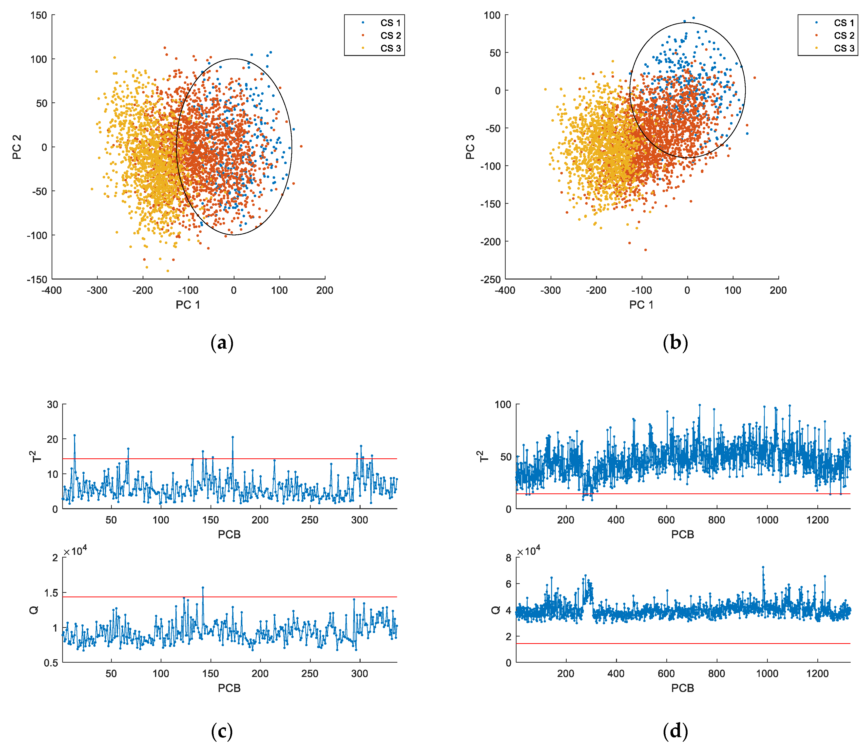
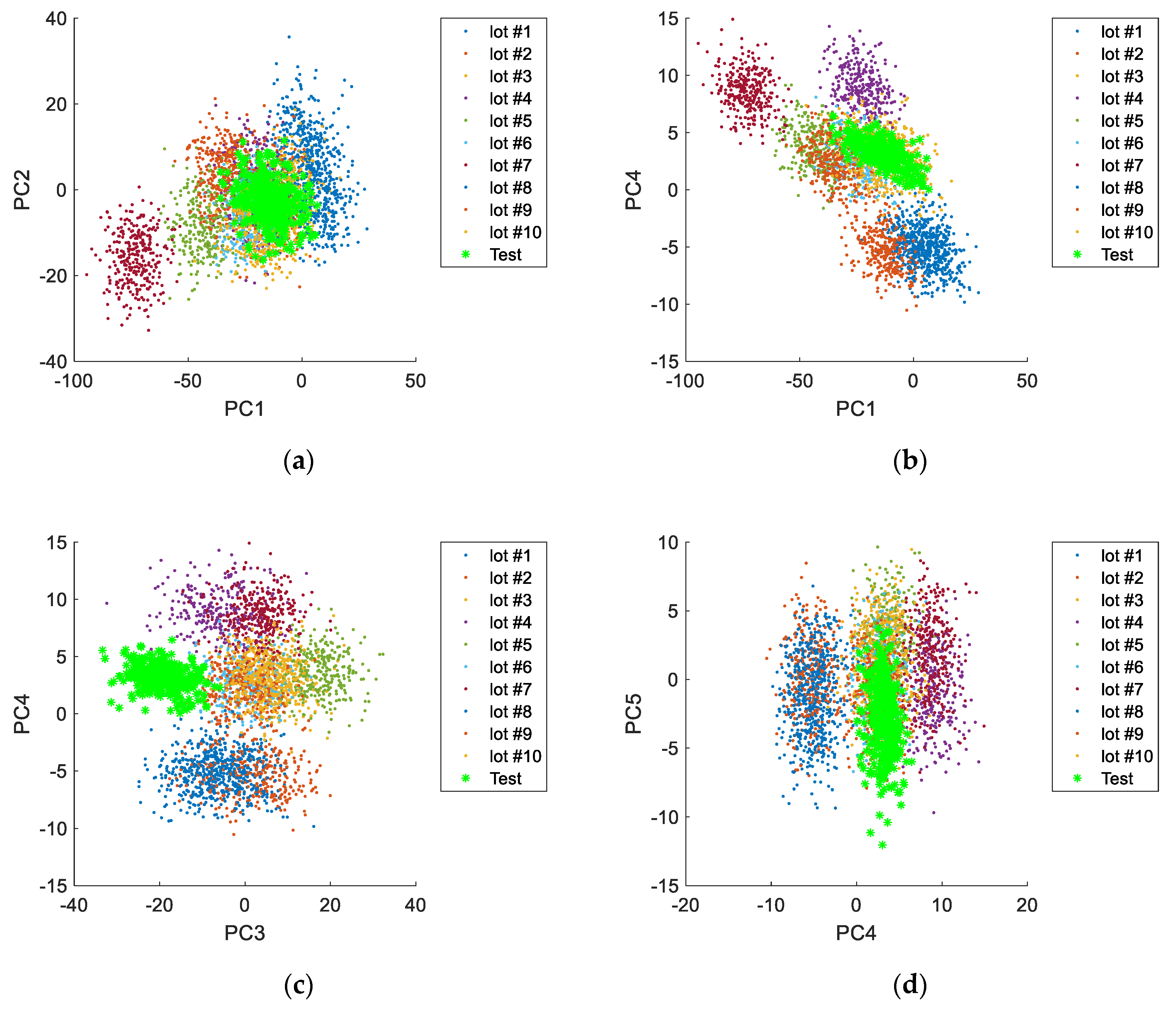
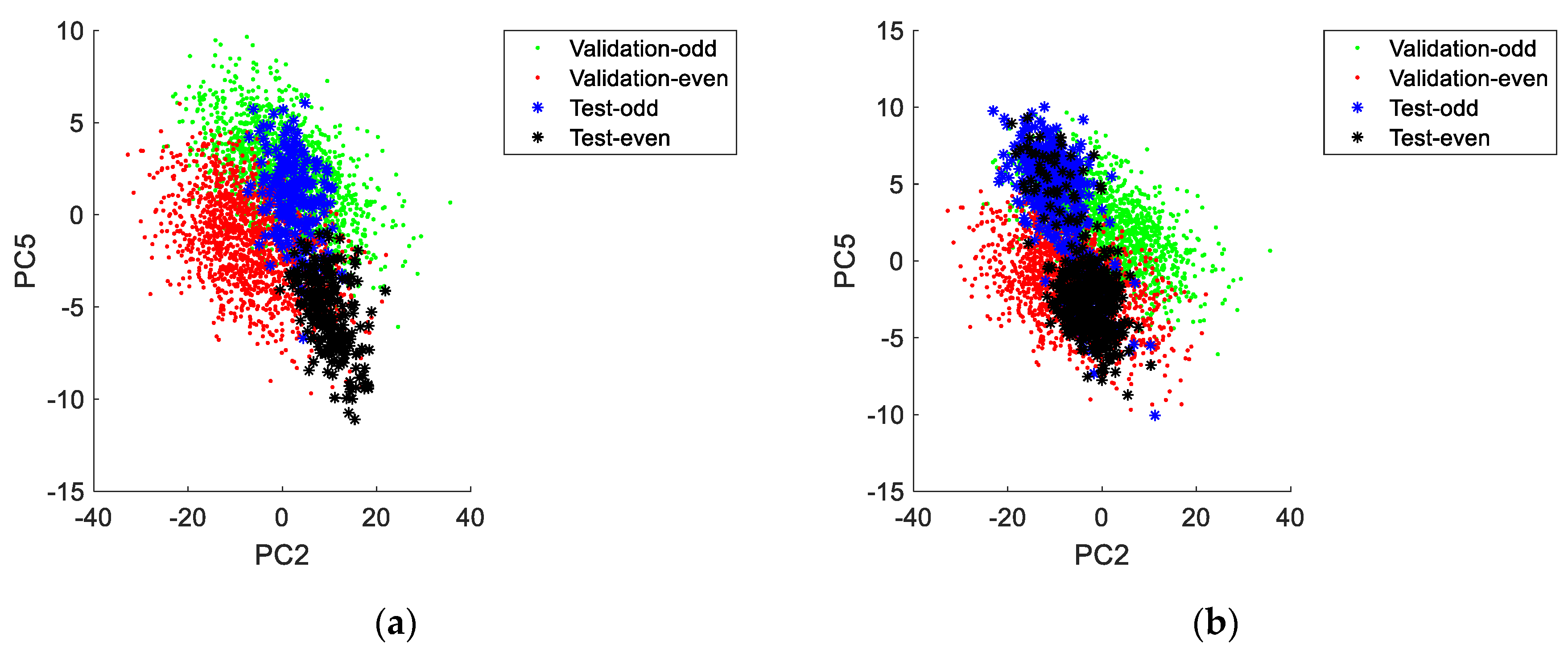
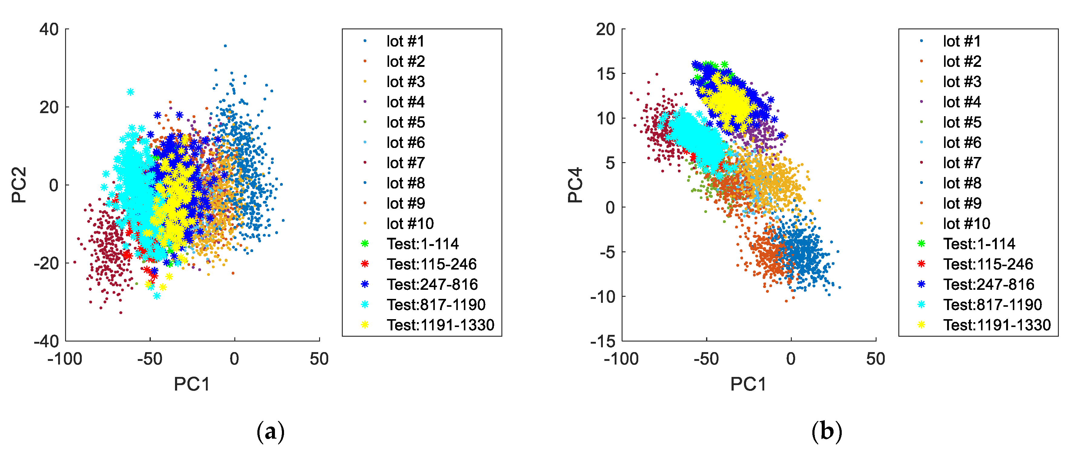
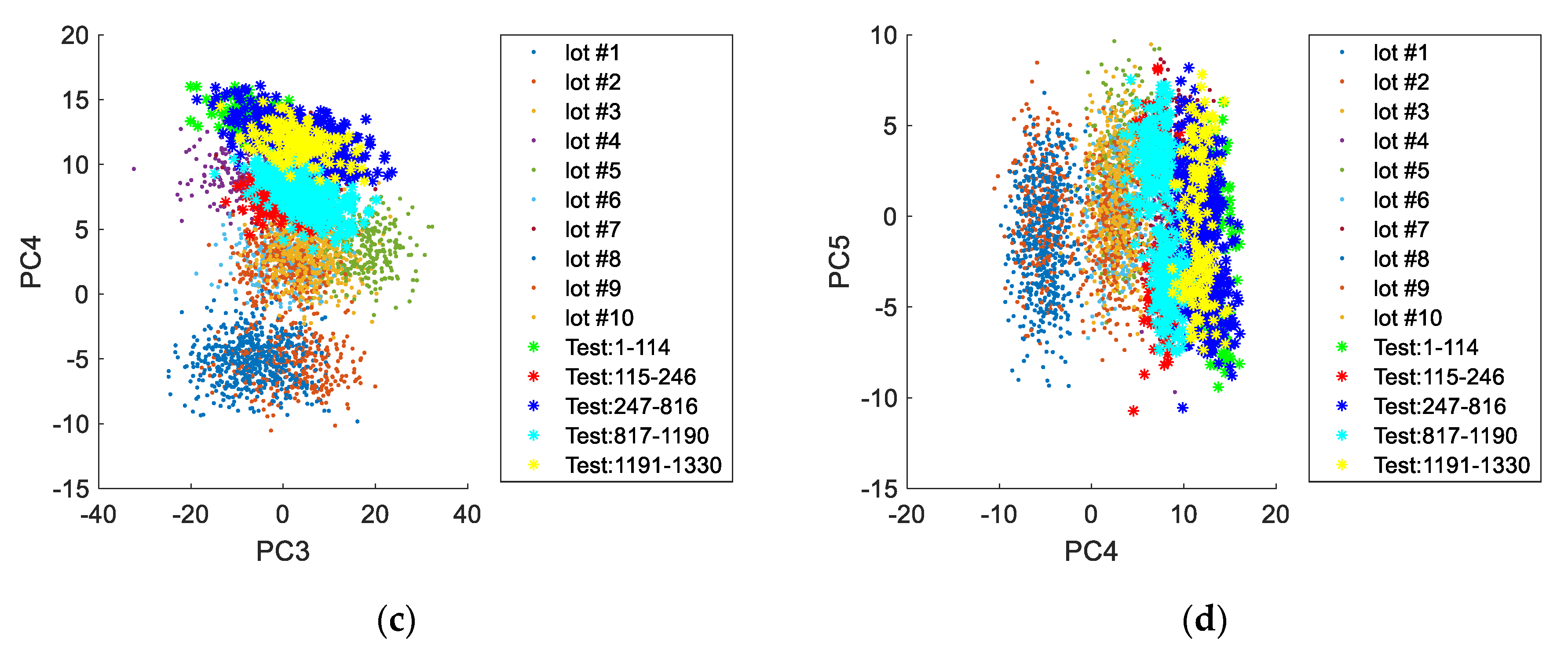
For a better understanding of the problem under analysis,
Figure 1a,b represent the scores for the first three principal components (PC1, PC2 and PC3) for several datasets collected for the production of the same product, all of them regarding NOC conditions. Given the large number of variables involved, we opt to present just these three scores, that represent a significant portion of the overall variability (from the properties of Principal Component Analysis, they are the three linear combinations with maximum explanation power of the variability presented by the original variables; see [
50,
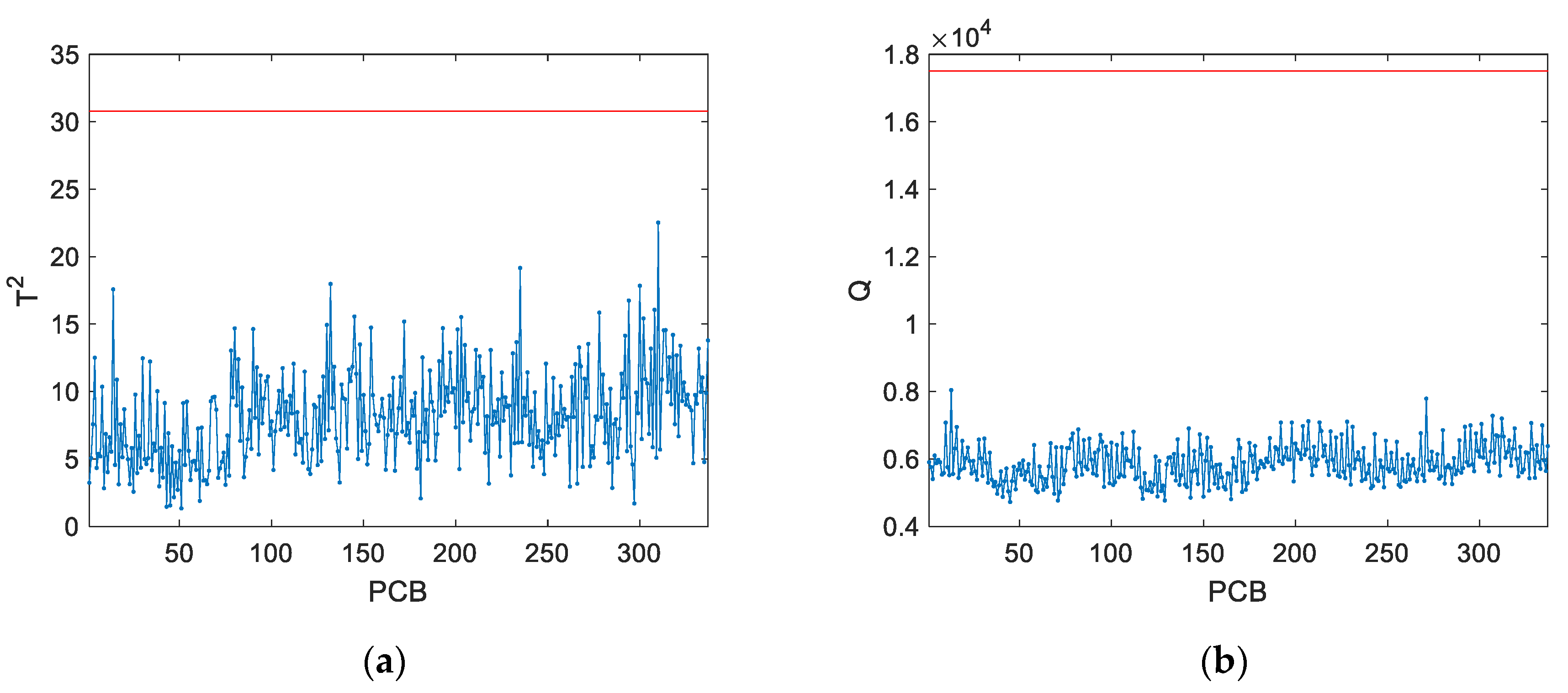
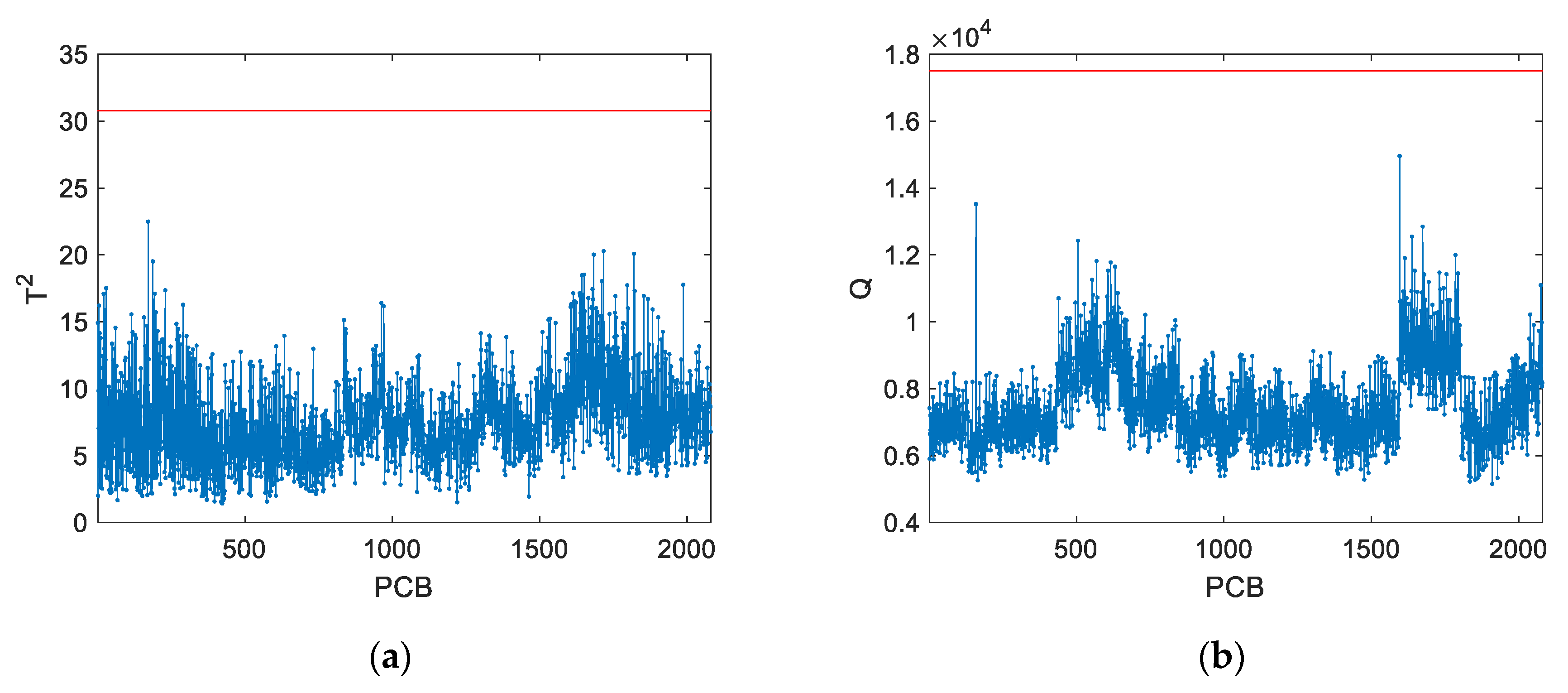
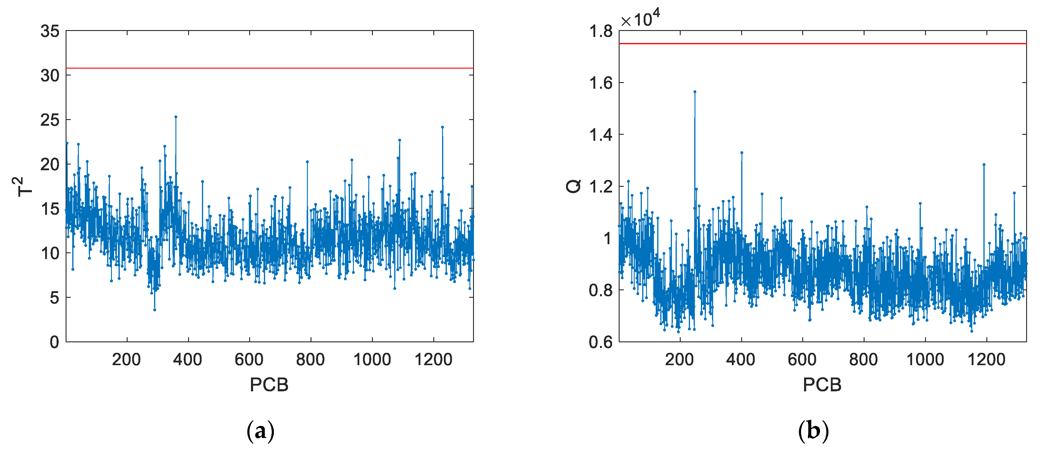
51]) and are enough to establish the picture we want to convey at this point. Each point concerns a PCB, and these points, as stated above, arise from the reference dataset (CS1) and other two datasets collected afterwards at different periods, also regarding normal operating conditions. All observations should therefore be considered “normal”, as confirmed by process experts. Conducting a Phase 1 analysis of the reference NOC dataset (CS1) it is possible to conclude that the process is stable. This can be confirmed by analyzing
Figure 1c, where the two multivariate monitoring statistics fall in general within the region limited by the Phase 1 control limits (more details on these monitoring statistics are presented in
Section 4). This historic reference dataset can therefore be used to setting up the multivariate control limits from conducting the monitoring activity of future incoming PCBs. However, from the plot in
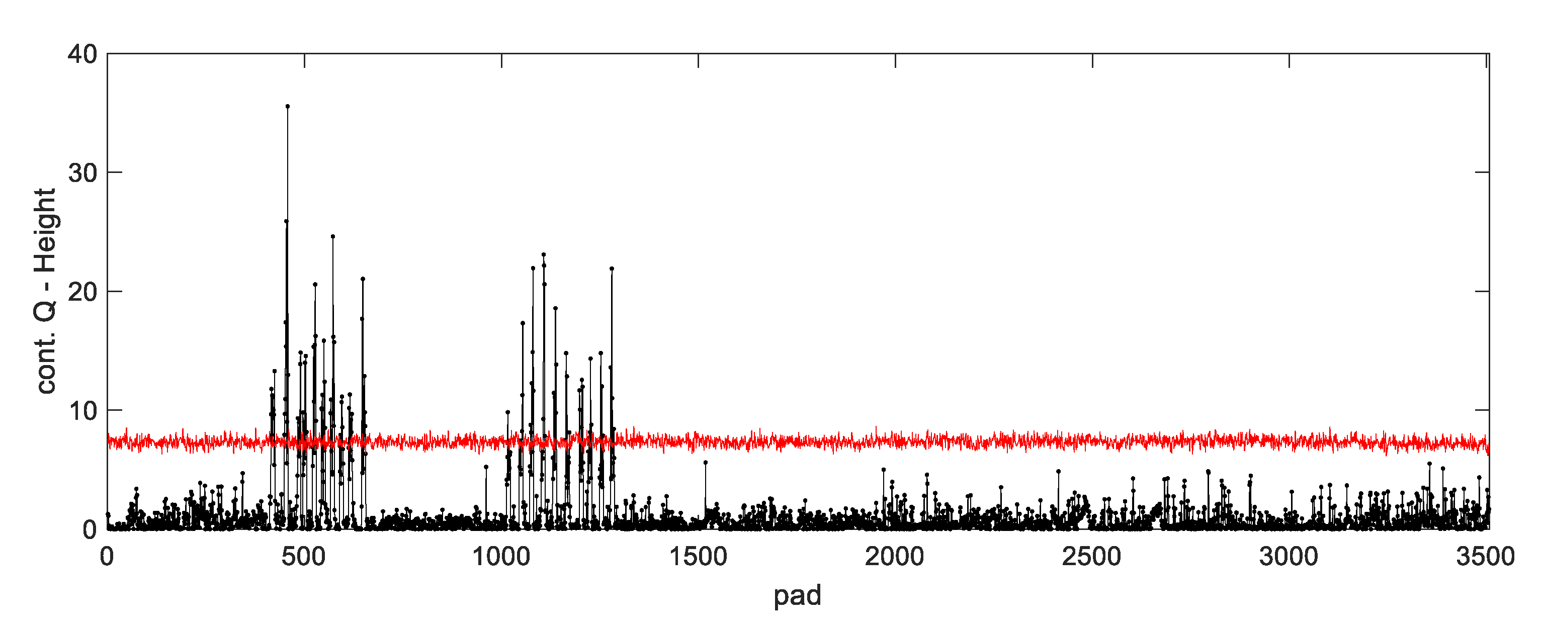
Figure 1a,b, it is clearly visible that many alarms are expected to be issued when applying these control limits to data from future PCBs. This can actually be confirmed by analyzing
Figure 1d, where the SPM charts developed using CS1 were applied to dataset CS3, resulting in sustained alarms being issued by the two control charts. Therefore, implementing any SPM methodology based on the information strictly inferred from the historical dataset will inevitably result in frequently signaling as faulty PCBs that are perfectly good, making this activity, as it is currently conducted, of very limited value.
The fundamental reason causing the situation described above is the limited information about process variability that can be extracted from a dataset representing a stable period of NOC operation—the reference dataset does not reflect the whole of common cause variation sources, but just a small part of it.
Fortunately, the reference NOC dataset is not the only source of information about common cause variation available.
In fact, the engineering team has been accumulating knowledge over time about the “common” causes of variability that lead to such false alarms, by analyzing case by case what is causing them. The root causes regard aspects that are very common and perfectly normal and expected in process operations, such as slight changes in the settings from different lots, automatic corrections and adjustments introduced by the assembly units, “normal” (or acceptable) tridimensional deformations in the boards fed to the process, rigid body movements (rotations, translations) of the boards as they move in the line, and other known specificities of the paste deposition tools. These aspects of variability are known and expected to happen over a long time frame, but not all of them will be, for sure, present in the initial stages of the process, or in any other single isolated period in the future.
Furthermore, the extensive process knowledge accumulated over time enables not only the identification of which phenomena may cause the variation patterns presented in
Figure 1, but also to know their magnitudes. The detailed analysis of past production runs where they took place, does provide information on the amount of variation associated with them. Therefore, besides the reference dataset, there is also information available about the
long term structural components of common cause variability (at least for the dominant modes of common cause variability), and their stochastic behavior (of which the reference dataset is a particular realization).
Bringing this extra engineering knowledge of common structural cause variation is fundamental to address the present problem rooted in the unavoidable underrepresentation of common cause variation in the reference dataset.
1.2. Proposed Methodology: Artificial Generation of (Common Cause) Variability (AGV)
In this work we introduce a Data Augmentation approach for enriching the reference dataset with structural common cause variation sources. Data is generated by conducting stochastic computational simulation of process behavior using rigorous mechanistic models for the dominant structural modes of common cause variation, whose conditions and parameters are described probabilistically based on data collected from industrial runs for other related assembly processes (dispersion) whereas the targets and settings are those of the current process (central tendency). The simulations will generate patterns of variation in the measurements respecting the physical constrains of the systems/products, leading to the same natural long term and short term correlations patterns found in real process data.
Ultimately, the proposed methodology is even able to create a frame of reference for starting the monitoring right from the onset of the production, using the variation patterns extracted from previous runs with other products (as shown in
Section 5). We call it
conditionally expected common cause variation, i.e., the expected variability under normal operating conditions,
conditioned on all the past data and knowledge extracted over the years from data regarding the production of related products.
Together with the solution for the unwelcomed false alarms, the proposed methodology also brings new diagnostic tools: the variation from the different simulated phenomena is usually well captured by specific principal components. Therefore, once a potential fault is detected the analysis of the scores my reveal a possible mechanism underlying its origin (the one connected to the principal component where the deviation is more noticeable). Other causes can be explored by other diagnostic tools, such as residual analysis and contribution plots.
The aforementioned concept of conditionally expected common cause variation differs from Shewhart’s original perspective, but is still inspired in it. It requires and builds up on extensive knowledge about the process physics and accumulated data. As Industry 4.0 takes place, the evolution of Digital Twining technology is likely to create similar opportunities to use accurate models of the process, namely for process monitoring as proposed in this article.
The present article is organized as follows. In
Section 2, a brief description of the process and datasets to be analyzed is provided. Then, in
Section 3, we introduce in detail the proposed data augmentation methodology (Artificial Generation of common cause Variability, AGV). The monitoring scheme based on the augmented NOC dataset is described in
Section 4. The results from the application of the proposed data augmentation methodology for process monitoring to several real world industrial dataset are presented and discussed in
Section 5.
Section 6 further extends the discussion of results and their consequences. Finally, in
Section 7 we provide a brief summary of the main advantages and limitations of the proposed methodology and refer to future work to address these limitations and make the approach more sensitive to localized faults affecting a relatively small number of elements.
2. Process Description
The process considered in this work regards a surface mount industrial unit (Bosch Car Multimedia Portugal), composed by several lines where electronic components are attached to PCBs through reflow soldering. In this process, SPDs are accurately placed in designated points of copper PCBs that will be used to fix and functionalize electronic components further ahead in the assembly line, through reflow soldering under a predefined temperature profile. Several thousands of SPDs are set in place, with a cycle time that can achieve approximately 20s. The resulting PCBs with printed SPDs are subject to 100% 3D Solder Past Inspection (3DSPI). This technology has been a pillar for process monitoring and improvement in this plant, and will be further explored in this work. 3DSPI generates, for each single SPD printed in the pad, a full 3D profile, retaining 5 features for analysis: area (a), height (h), volume (v), offset in the X-direction (x) and offset in the Y-direction (y).
In this work, we consider the production of one specific product from which 3507 SPDs (we will also use the designation of “pads” to refer to such SPDs) are monitored, totaling 3507 × 5 = 17,535 variables to be handled. Three datasets are available and will be used in this study to test the proposed approach: CS1 contains information for 337 NOC PCBs and is used to validate the AGV methodology and confirm/tune some of its parameters; CS2 and CS3, contain 2080 and 1330 PCBs, respectively, mostly regarding good products, but also containing some PCBs with a few faulty pads. CS2 and CS3 will be used to further test the proposed methodology.
3. Artificial Generation of (Common Cause) Variability (AGV)
The proposed methodology for Artificial Generation of (common cause) Variability (AGV) aims at completing the reference dataset with the long term dominant sources of common cause variability that, from engineering knowledge, are known to exist. This is done by simulating the printing of solder paste deposits in Printed Circuit Boards (PCB) under situations where the dominant sources of common cause variation span their normal range (as extracted from the analysis of historic data from production runs of related products). The simulations are based on accurate mechanistic/first principle models and reproduce the effects of underlying common causes on the 3DSPI measurements of solder paste deposits: area (a), height (h), volume (v), offset-X (x) and offset-Y (y). As part of the common cause variation is introduced when different lots of the same product are produced while others are active during the production of a given lot, the AGV module also accounts for both inter-lot, intra-lot and pad specific variability.
During the process simulation, the AGV module generates data for
L lots with
B PCBs each, where each PCB is composed by
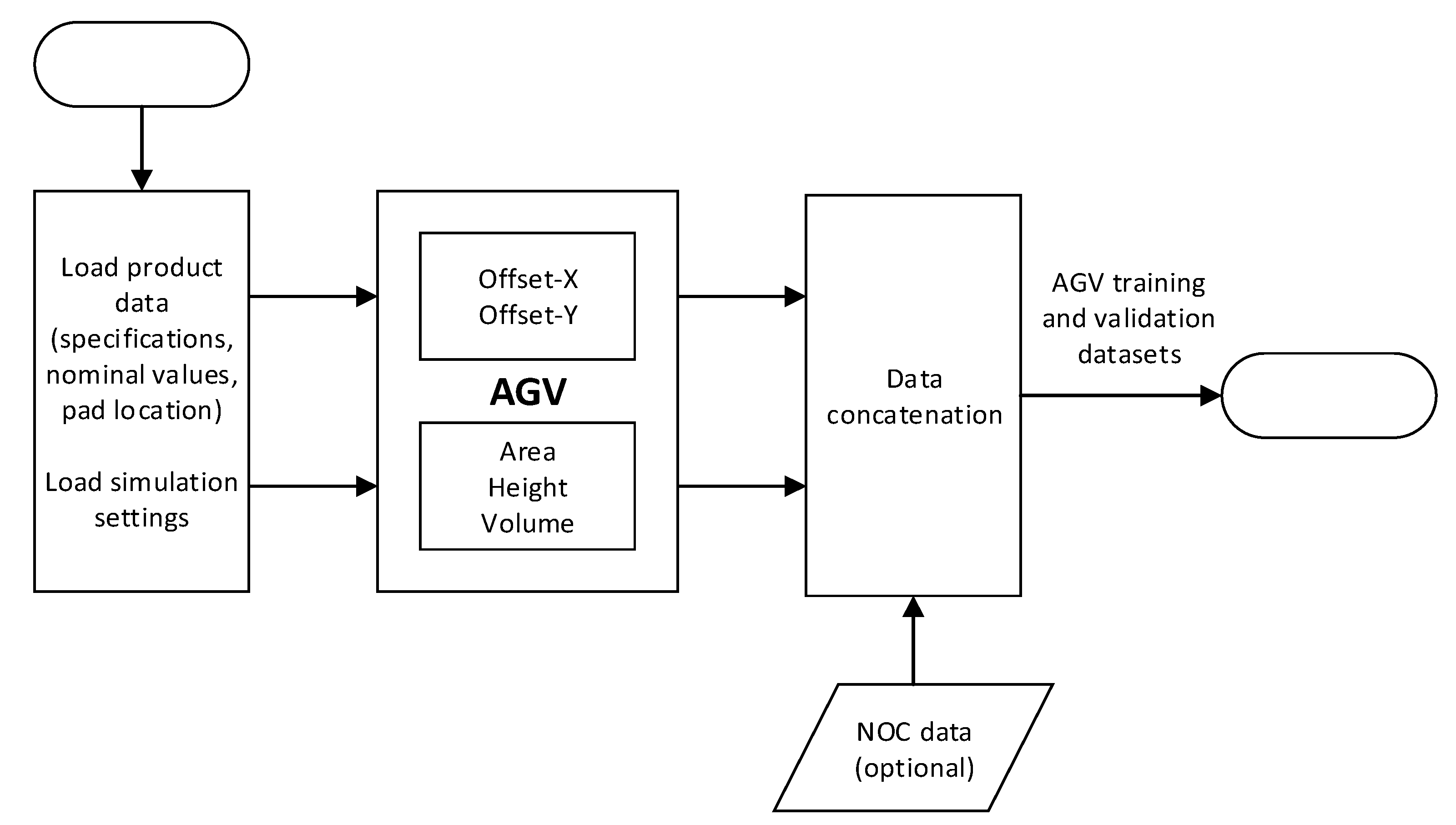
P pads (a pad is a small part of the PCB where SPD should be placed). A more comprehensive description of the simulation settings for each of the variability sources are provided in the following subsections. A schematic representation of the AGV module is presented in
Figure 2.
The basic inputs of the AGV module are the nominal values and tolerance limits for the measured parameters (
a,
h,
v,
x,
y) and the geometrical coordinates of each pad (
Table 1). Based on this information, the allowed variability given the existing tolerance limits is estimated by,
This parameter is analogous to the standard deviation and is based on the fact that, for normally distributed data, 99.73% of the data falls within the ±3 sigma interval.
Along with the PCB’s tolerance specifications, the user can also define a set of tuning parameters (
Table 2) that allow for the full configuration of the simulated conditions of the printing process. The relationship between the tuning parameters and the process phenomena is discussed in the following subsections. It is expected that, in future applications for the same lines and for related products, the settings for most of these parameters will not change. However, the need for some tuning can be readily assessed after collecting the 3DSPI measurements from the first few products.
3.1. Common Cause Variation Affecting Offset-X and Offset-Y
The relative location of the pads can be affected by rigid body translations and rotations of the PCB. Furthermore, offsets in the y-coordinate (offset-Y) can also be attributed to the printing direction of the squeegee.
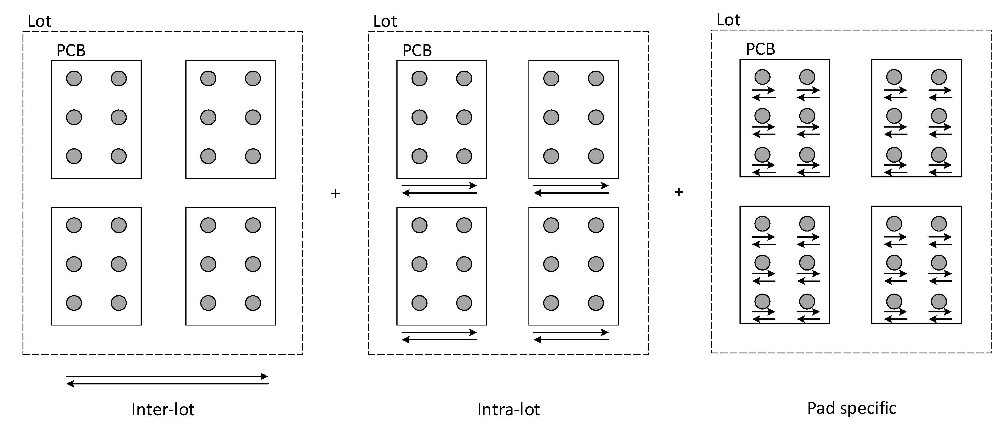
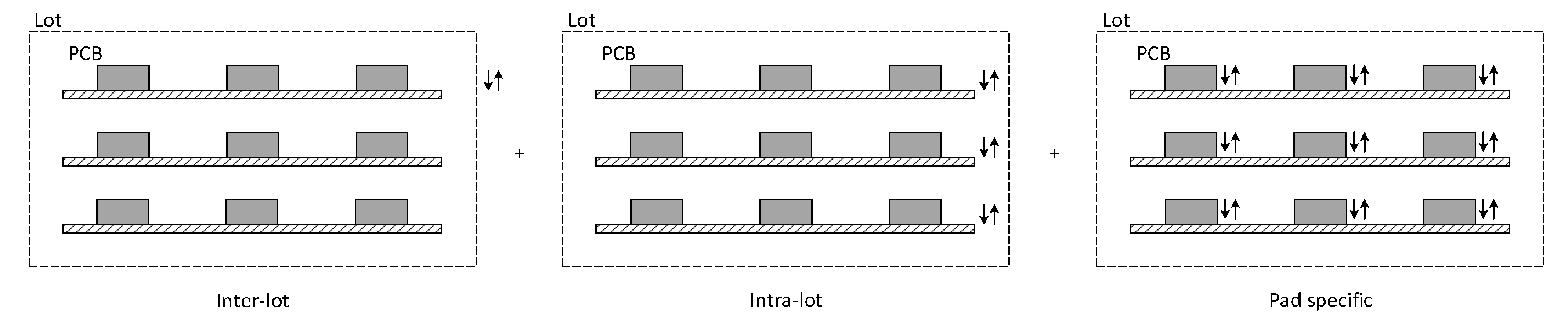
The translation effects are identical for both offset-X and offset-Y. For the sake of brevity, only the case of offset-X is described. To simulate the rigid body translation effect (
Figure 3), we considered that it can be split into three components. These are relative to:
- (i).
An overall deviation that is common to all PCBs within a lot—inter-lot variation: ;
- (ii).
A local deviation that affects all pads in a PCB—intra-lot variation: ;
- (iii).
Unstructured deviations for each pad—pad specific variation: .
In these simulations,
,
and
are generated by taking random draws from the standard normal distribution. The fraction of total variation attributed to each component is determined by the scaling factors
,
and
. These scaling factors must fall between 0 and 1 and are further restricted to comply with:
Thus, the sum of all components amounts to one unit of allowed variance. Finally, the components are scaled by the allowed variance , where is the allowed standard deviation for the offset-X of the p-th pad and is a scaling factor.
Following the above definitions, the translation effect on the offset in the
x-coordinate for the
p-th pad of the
b-th PCB of the
l-th lot (
) is given by (
Table 3):
Likewise, the translation effect on the offsets in the
y-coordinate (
) are simulated by (
Table 3):
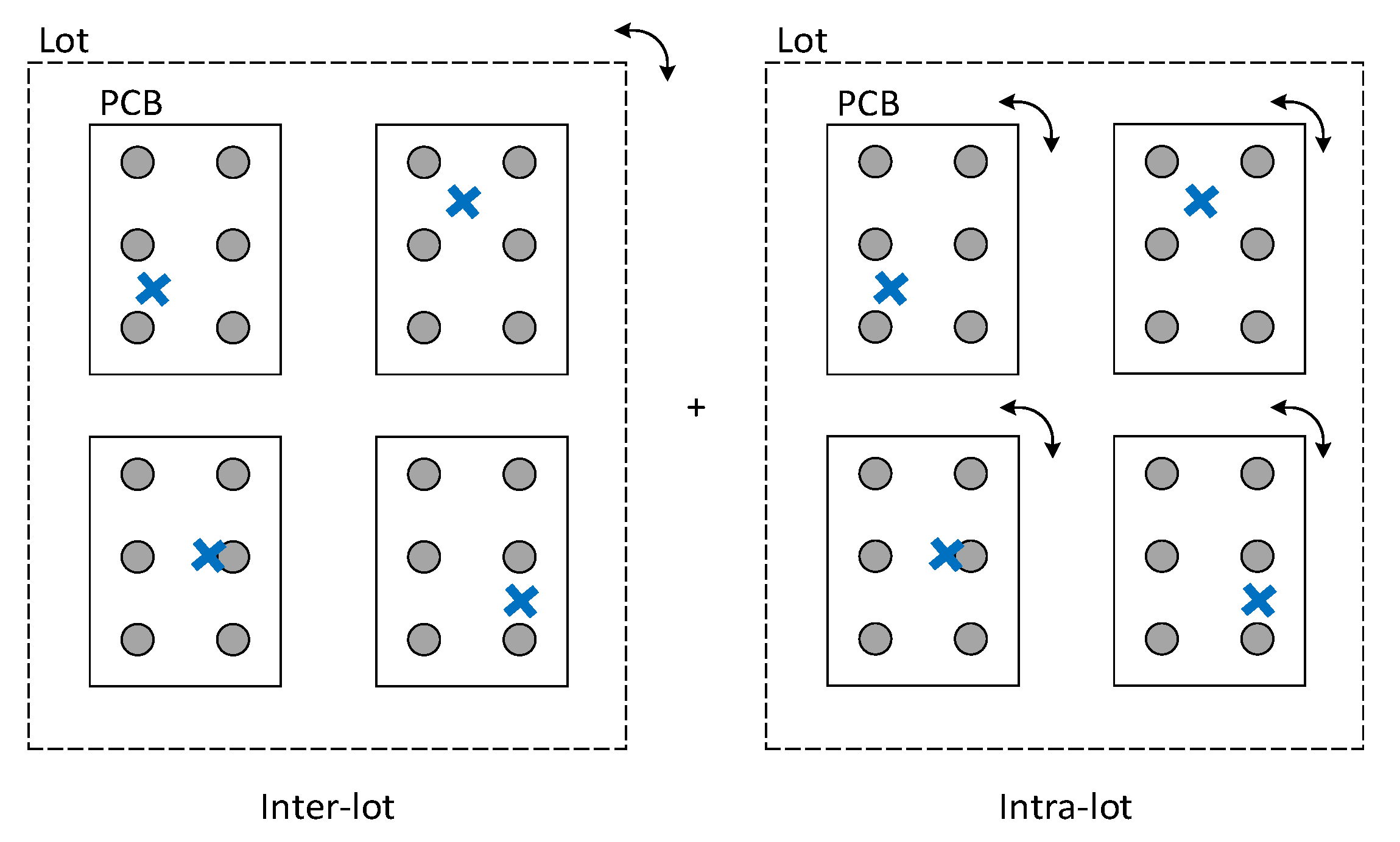
The rigid body rotation effects (
Figure 4), are taking into account by simulating rotations in the PCB with different centers and magnitudes. This rotation can be further decomposed into:
- (i)
An inter-lot rotation angle that affects all PCBs within a lot - inter-lot variation:
- (ii)
An intra-lot rotation angle that adds specific variation to each PCB—intra-lot variation: .
The
and
variables are generated from the standard normal distribution and scaled by the allowance rotation angle
, divided by 3 to ensure that the rotation angle falls, with high probability, between
. Furthermore, the amount of variability attributed to the inter-lot and intra-lot components is defined by the scale factors
and
, which are between 0 and 1 and comply to the condition:
Based on this, the rotation angle of the
b-th PCB of the
l-th lot (
) is computed as,
The rotation matrix is subsequently obtained by,
The center of rotation is randomly generated for each PCB using the uniform distribution. More specifically, the x-coordinate for the center of rotation () is taken from the uniform distribution on the interval , where is a vector with the x-coordinates of each pad. Similarly, the y-coordinate of the center of rotation () is generated from the uniform distribution in the interval , where is a vector with the y-coordinates of each pad.
Using the above information, the rotation effects on the offset-X,
, and offset-Y,
, for the
p-th pad of the
b-th PCB of the
l-th lot, are determined by (see
Table 4.):
Along with the translation and rotation effects, the offset-Y is also affected by an additional systematic bias caused by the printing direction of the squeegee (the squeegee is the device that pushes the solder past deposits placed on the top side of the stencil towards the existing apertures in the stencil). This phenomenon leads to a positive deviation in the offset-Y when the printing is performed in one direction and a negative deviation when the printing direction is reversed. Without loss of generality it is assumed that PCBs with an odd index
b are printed in the direction of increasing
y-coordinates. Conversely, PCBs with an even index
b are assumed to be printed in the opposite direction of decreasing magnitude
y-coordinates. To simulate the squeegee effect on offset-Y (
;
Table 5), the allowance deviation that can be caused by the squeegee is defined by
and its impact is alternated with the PCB index. Furthermore, to account for local random variation, for each PCB, the allowance deviation is multiplied by a random variable with uniform distribution in the interval [0,1].
Finally, the offset-X (
) and offset-Y (
) are determined by summing all effects:
where
and
are the nominal value for the offset-X and offset-Y of the
p-th pad.
3.2. Common Cause Variation Affecting Height
The height of solder paste in each pad is affected by the solder mask and the squeegee’s action. The effect of the solder mask translates into systematic deviations across all PCBs in the same lot (because the same mask is used in each production lot). The allowed deviation due to the solder mask is here defined by
. Furthermore, its impact on the height is simulated through (
Figure 5):
- (i)
An overall component that affects all PCBs in a lot—inter-lot variation: ;
- (ii)
A specific component for each PCB—intra-lot variation: .
For both cases,
and
are generated from the standard normal distribution. The
and
factors scale the contribution of each component. These factors are between 0 and 1 and conditioned to:
As the total variability of the height is greater than that caused by the solder mask, the remaining variability is added as a specific component for each pad,
. Following these considerations, the solder mark effect on the height of the
p-th pad of the
b-th PCB of the
l-th lot (
) is computed as follows (see also
Table 6):
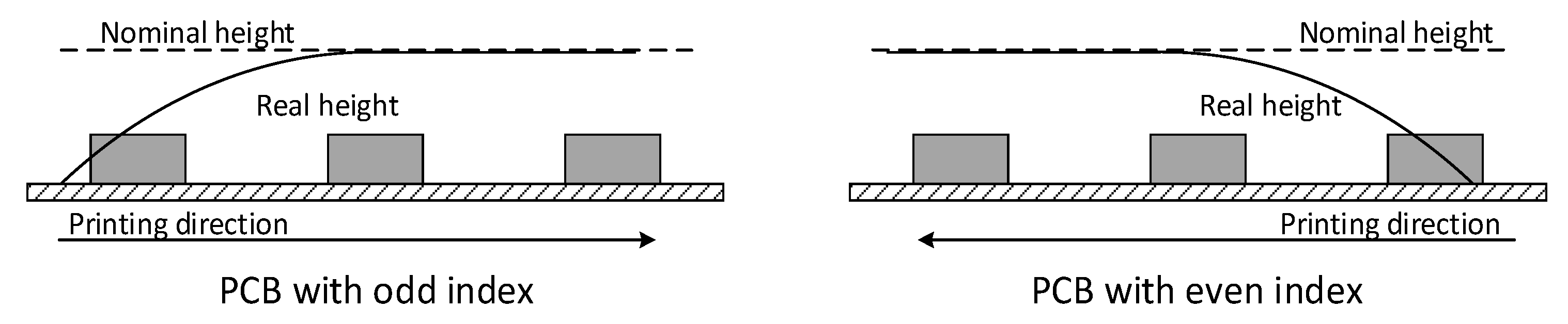
As in the case of the offset-Y, the height is also affected by the printing direction of the squeegee. This effect relates to a progressive increase in the pressure of the squeegee. At the beginning of the printing process, the pressure is low and thus the heights are typically lower than intended. As the printing progresses, the heights reach the intended nominal values. The same applies when the printing direction is reversed, but now affecting the pads on the other extreme of the PCB (
Figure 6). To be consistent with the squeegee effect on the offset-Y (see
Section 3.1), it is considered that PCBs with an odd index
b are printed in the direction of increasing
y-coordinates, while PCBs with an even index are printed in the reversed direction.
To systematically address both printing directions, the original
y-coordinate of the pads is transformed into an equivalent distance, related to the point where the printing beginnings, by:
where
is a vector with the
y-coordinates of each pad,
p is the pad of interest and
b is the PCB index. Based on this, the influence of the squeegee in the height (
) is modeled through an exponential decay function (
Table 7):
where
is the maximum allowance deviation,
is a length constant and
is a random variable following
. Process knowledge indicates that the deviation in
is more pronounced in the first third of the PCB (i.e., until
). Thus, by considering that for
the deviation in
is reduced to 13.5% of the allowance deviation, the length constant is set to:
The final value for the height of each pad (
) is determined by summing the solder mask and squeegee effects:
3.3. Common Cause Variation Affecting Area
The area common cause variation can be conceptually subdivided into three components representing (the structure of each component is analogous to
Figure 3):
- (i).
Inter-lot deviation that impacts all pads of all PCBs in the same lot—inter-lot variation: ;
- (ii).
Intra-lot deviation that affects all pads in each PCB—intra-lot variation: ;
- (iii).
Local variability that affects each pad—pad specific variability: .
The random part of each component (
,
and
) is drawn from the standard normal distribution and scaled by the allowed standard deviation of each pad’s area (
) using a scaling factor for the total variance (
). Furthermore, the contribution of each component is codified by the scaling factors
,
and
, which are between 0 and 1 and are subject to:
Therefore, the final variance for the area of each pad is
. Following these definitions, the values for the area (
) are obtained by (
Table 8):
3.4. Common Cause Variation Affecting Volume
The volume of solder paste deposit in each pad (
) is considered to be proportional to the product of area (
) and height (
):
where
is a correction constant (
Table 9). For the case studies considered in this article, three different values for
were observed. However, it was not possible to establish a relationship between this parameter and the pads’ location or geometry. Therefore, in the absence of further prior information, it is suggested that
is estimated using the nominal values for volume, area and height such that:
4. Multivariate Statistical Process Monitoring Based on Principal Component Analysis (MSPM-PCA)
In the previous section, details were given regarding the artificial generation of common cause variability for the SPD printing process in a Surface Mount Technology (SMT) production line. This is done in the AGV module, and the simulation outputs for area (a), height (h), volume (v), offset-X (x) and offset-Y (y), are used to augment the reference NOC dataset, enriching it with a wide overage of common cause variation modes. The augmented NOC dataset can then be used to set up a multivariate statistical process monitoring scheme, which in the present case is based on principal component analysis (PCA).
PCA is a latent variable methodology that decomposes the original data matrix,
, with
observations and
variables, as:
where
is a
matrix of PCA scores,
is a
matrix with the PCA loadings,
is a
matrix of residuals and
is the number of retained principal components (PC). As PCA is scale-dependent, the data matrix
is usually standardized or “autoscaled” to zero mean and unit variance.
The principal components of PCA are monitored by the Hotelling’s
as proposed by [
52,
53],
where
is a
vector with the current observations,
is a diagonal matrix with the first
eigenvalues in the main diagonal. If the process follows a multivariate normal distribution, then the upper control limit (UCL) for
can be computed as [
54,
55]:
where
is the upper
-percentile of the
F distribution, with
and
degrees of freedom.
The complementary residuals’ subspace is monitored through the
Q-statistic based on the squared prediction error (SPE) of the residuals,
[
53]:
where
is the projection of
onto the PCA subspace. The UCL for this statistic is usually determined by [
53,
56]:
with,
where,
is the upper
percentile of the standard normal distribution.
Due to deviations in the model assumptions, the theoretical control limits for the PCA monitoring statistics are often found to be inaccurate. Therefore, it is often preferable to set the control limits by adjusting a scaled
distribution to the empirical distributions of
and
[
57,
58,
59], leading to:
where
is a weighting factor and
is the effective number of degrees of freedom for the
distribution. Both values are obtained by matching the moments of the
distribution with those of the empirical distributions obtained from NOC data, leading to
and
, where
is the sample variance and
the sample mean of the monitoring statistic.
Under the PCA framework, fault diagnosis can be performed by resort to contribution plots [
60,
61,
62,
63]. In this context, the contribution of the
i-th variable for the
and
statistics are computed as [
62,
64],
where
is the
i-th row of
and
is the
i-th element of
. The theoretical control limits for each
and
can be found in Refs. [
62,
64]. Alternatively, the scaled
approximation described before can also be used.
5. Results for the Implementation of AGV in an Industrial SMT Process
The results presented next regard the printing of solder paste deposits in PCBs composed by 3517 pads. For each pad, measurements for five parameters are collected: (i) area; (ii) height; (iii) volume; (iv) offset-X; (v) and offset-Y. For monitoring purposes, only 3507 pads are considered since the remaining pads are associated with atypical shapes for which the accumulated historic data is not yet enough to set up the AGV module parameters; they are also known to produce unusual offsets in x- and y-coordinates even in NOC. Consequently, the total number of variables under monitoring is m = 3507 pads × 5 parameters = 17,535 variables.
To analyze the characteristics of the proposed AGV module, three real datasets are considered in this study. The first dataset (CS1;
Section 5.1) corresponds to NOC data and is composed by 337 PCBs. The second dataset (CS2;
Section 5.2) contains 2080 PCBs taken from a different production run. Similarly, the third dataset (CS3;
Section 5.3) has 1330 PCBs taken from a third production run. The CS2 and CS3 datasets are mostly composed by normal PCBs, but also contain some faulty PCBs. Furthermore, due to structured common cause variation in the process, the operational state of the three case studies is typically distinct.
In this study, the PCA model is trained using only simulated data generated by the AGV module with the values for the tuning parameters presented in
Table 2. No data from the process was employed for building the PCA model or setting up the monitoring charts (they can be also considered, for this reason, pre-control charts). 20 lots with 300 PCBs in each lot were generated in the AGV module. Ten of these lots were used to build the PCA model (training dataset). The other ten lots were used to set the control limits by adjusting the empirical distributions of the monitoring statistics (validation dataset). The control limits were set to a false alarm rate of 0.01. Although we only present here the results for one set of the 20 lots, several replicates were analyzed leading to similar results.
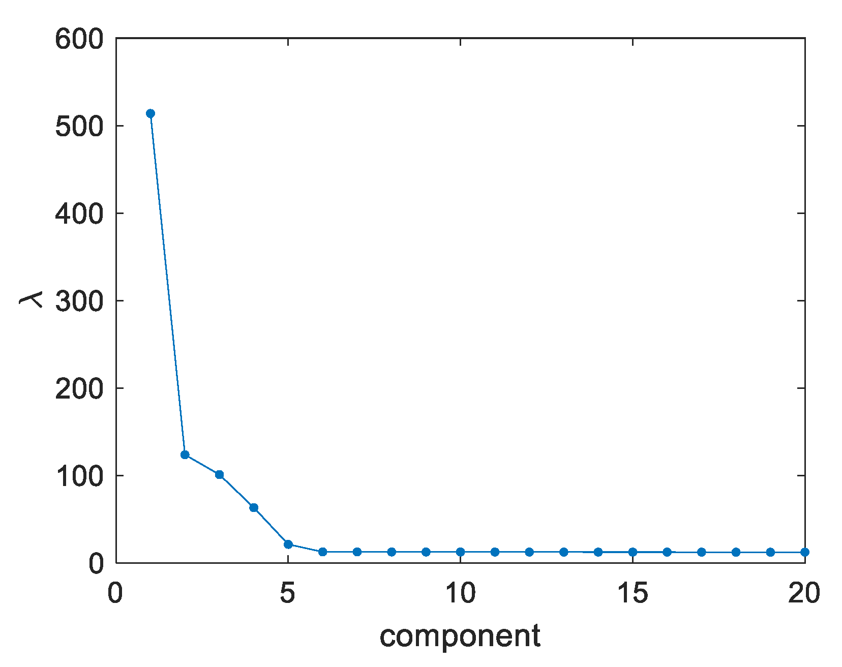
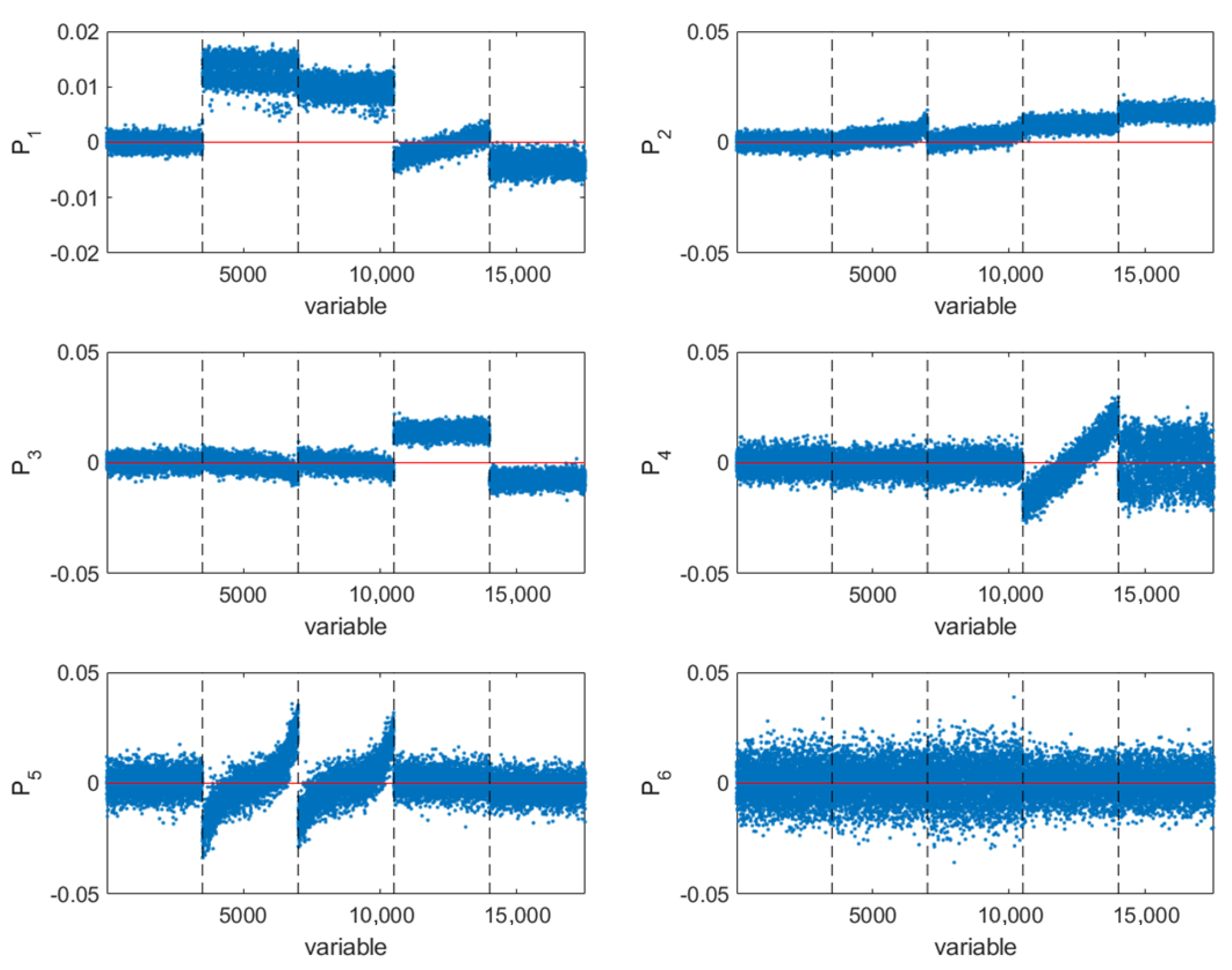
From analysis of the scree plot in
Figure 7, the number of retained principal components was set to 5. By further inspection of the PCA loadings (
Figure 8) it is verified that the first five components have a close relationship with known phenomena. PC1 describes the relationship between heights and volumes. This PC also shows that the variation in the SPD’s height and volume is related to the pads’ location in the PCB. PC2 and PC3 explain the rigid body translation effects in the PCBs, while PC4 describes the rotation effects. PC5 is related to the squeegee effect in the heights and its propagation to the volumes. For this reason, PC5 is also related to the printing direction. As for the remaining PCs, they are mostly associated with relationships between areas and volumes of different SPDs. However, since the variation in the area is assumed to be independent from pad to pad, each one of them tend to generates a different PC. Therefore, many PCs are generated by this effect (note that there are over three thousands of pads involved in this mechanism). This justifies why the first 5 PCs explaining the most relevant structured phenomena for process monitoring contain less than 5% of the total variance in the simulated data. However, the monitoring procedure still comprises all the process variation: both the variation captured by the first 5 PCs (through the Hotelling’s
T2 statistic for the selected PC scores) and the complementary residual variation (using the
Q-statistic for the PCA residuals). Therefore, this asymmetrical distribution of common cause variability is consistent with the physics of the process and does not pose any problem or limitation for the monitoring scheme.
5.1. Analysis of Dataset CS1: NOC Data
The CS1 is composed by NOC data, and therefore it will be used to validate the AGV simulation module. By applying the PCA model to this dataset the score plots in
Figure 9 are obtained. The results show that the scores from CS1 do not fully overlap the scores from the simulated lots. This is visible in the plot of PC3 vs. PC4 (see
Figure 9c), and is an expected behavior since the inter-lot variability causes the lot to fall in a different region of the scores space. In this case, CS1 has lower scores in PC3 than the simulated lots. PC3 is related to translation effects in the PCBs, which implies that the PCBs in CS1 have a systematic translation in a given direction. Note however that some of the simulated lots have translations with similar magnitudes but on the opposite direction. As these inter-lot translations occur randomly and in either direction, we consider that the simulated data is still representative of real operation conditions. The different behavior across the lots is also visible for PC1 and PC4. Since both PCs are related with changes in offset-X and offset-Y, this indicates that the alignment of the PCBs in each lot is a critical factor in the final quality of the products. This information will be further explored in
Section 5.2 and
Section 5.3 to identify possible problems in the different datasets under analysis. As for the intra-lot variability, it is verified that the dispersion of the real data is similar to that obtained with the AGV module.
As for the control charts produced by the PCA model (
Figure 10), it is noticeable that the monitoring statistics are relatively low compared to the control limits. This happens because the PCA model was built using multiple lots, while the monitored data respects to a single lot operating in a well-defined and localized region, spanning only a small fraction of the operational NOC space.
One word of caution should be referred about the proposed approach, resulting from our accumulated experience on its application to real data. Although the proposed methodology decreases the chance of declaring a false alarm due to a change to another lot and solves the issue of false alarms that render classical monitoring methods useless, it also decreases the sensitivity to detect small deviations within a lot since a slightly deviating PCB may be treated as belonging to a different lot rather than being abnormal. This is a consequence of incorporating inter-lot variability in the AGV simulation scenarios.
Related to this issue, it was also noted that the Q-statistic is affected by the large number of monitored variables (m). In this case, there are 17,535 variables, but only 5 PCs are retained in the PCA model. These 5 PCs also explain a small fraction of the total variance (less than 5%), meaning that most of the variability of the data is monitored by the Q-statistic. In other words, the Q-statistic cumulates a large number of squared residuals with rather large variances. Thus, when a fault occurs, even with a large magnitude, it can suffer from dilution effect from the contribution of all residuals.
From the analysis of the dataset CS1, we can confirm that real NOC data fall inside the expected NOC envelop obtained from the AGV module. The dispersion characteristics of the CS1 lot in the PCA subspace are also similar to the simulated lots, which occupy different regions in the PCA subspace due to the expected (and simulated) inter-lot variability. These observations consubstantiate the rigor placed on the model development process, and provide confidence to the analysis of the remaining datasets using the PCA model developed in this section based on the simulated AGV data.
5.2. Analysis of Dataset CS2: Test Data (NOC and Faulty)
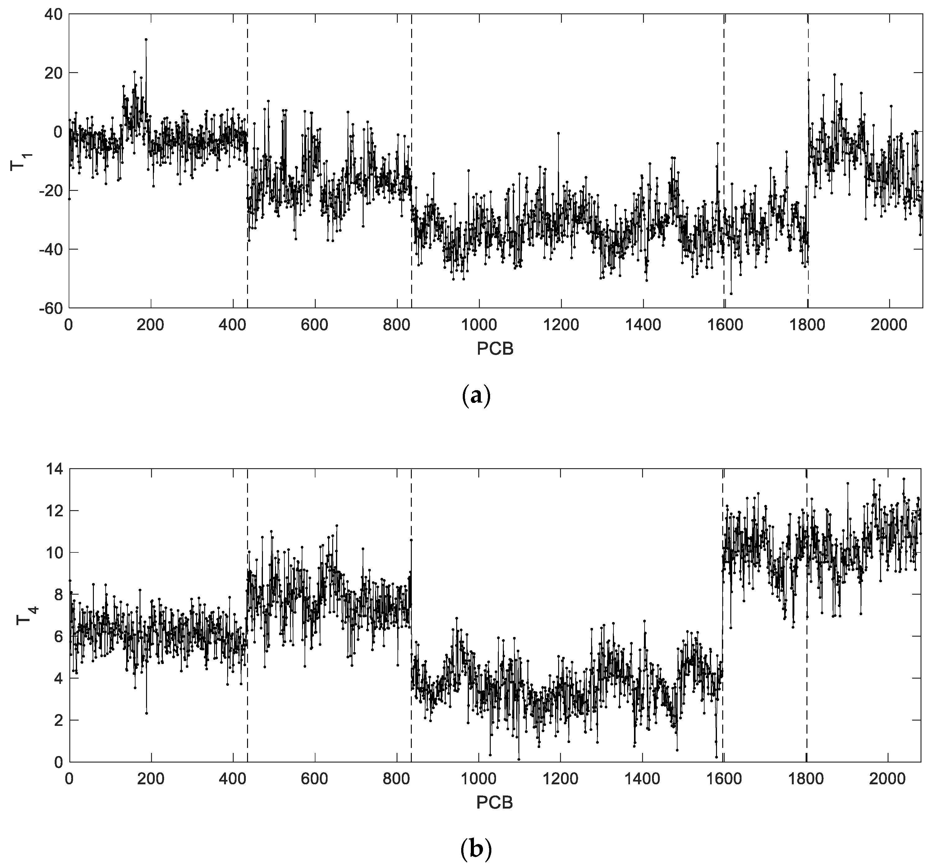
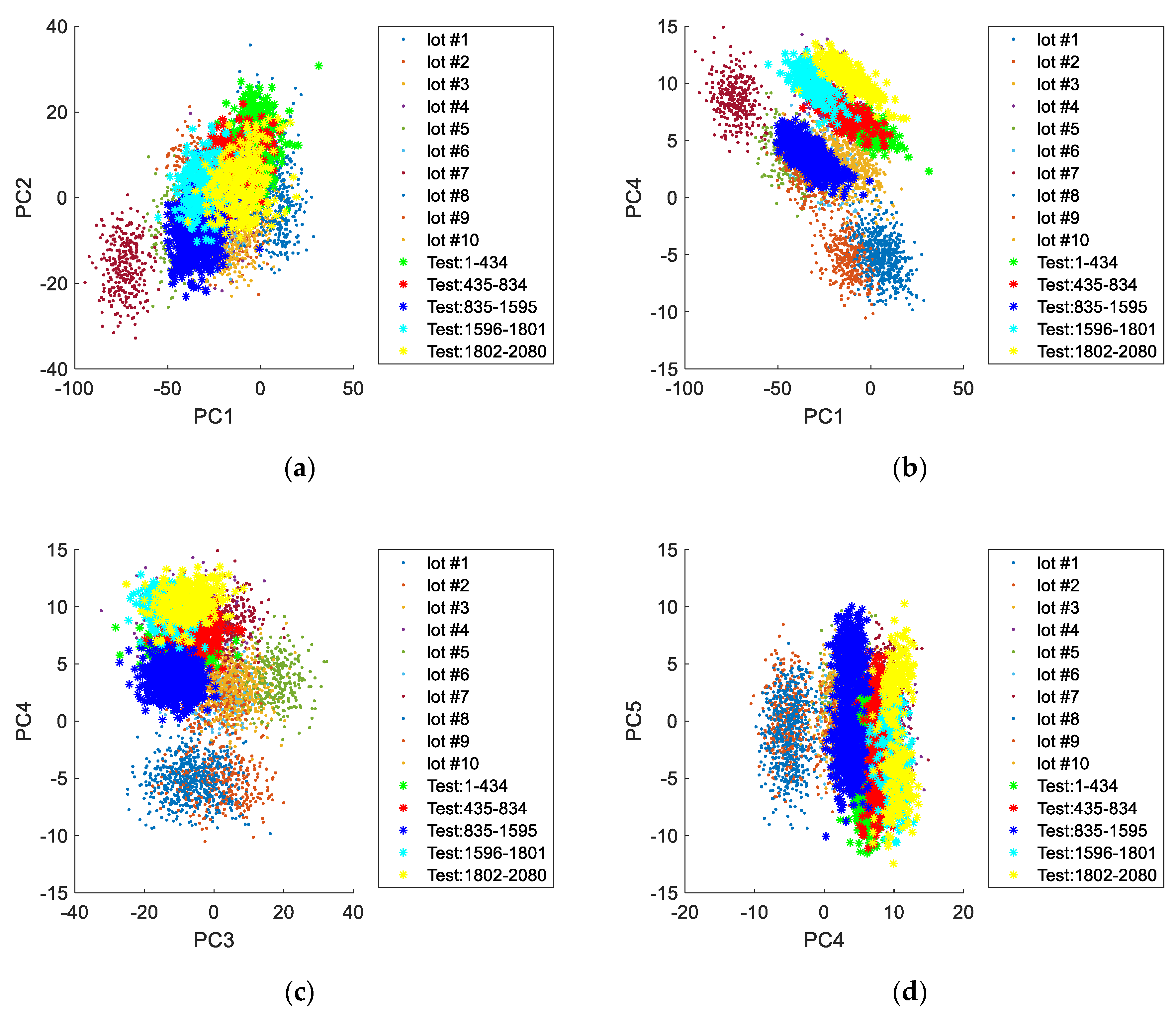
From analysis of the scores obtained for this case study (
Figure 11 and
Figure 12) it is apparent that this dataset is composed by at least five distinct operation periods. By comparison with the previously simulated validation lots, it is verified that all periods still fall within the typical operation conditions described by the PCA model applied to AGV data. It is also visible that each period resembles individual lots with specific characteristics. In this case study, a clear distinction in the printing direction is observed for some of the production periods. This phenomenon is more noticeable when PC5 is plotted against PC2 (
Figure 13).
By inspecting the control charts for this case study (
Figure 14), it is verified that all PCBs are marked as in-control. Nevertheless, it is noticeable that PCBs #159 and #1596 have atypical
Q-statistics. While for PCB #1596 most of the variables are within their tolerance specifications, PCB #159 present significant deviations in 151 variables. Therefore, PCB #159 is clearly a false negative. The deviations in the measurements of PCB #159 are passed to the residual subspace of PCA. However, since the critical residuals are only a small part of the sum of squared residual over all variables, they are not large enough to trigger an alarm. In spite of this, the contribution plots of PCA are able to identify the abnormal pads and parameters (
Figure 15). This result suggests that a monitoring statistic focused solely on the relevant residuals (i.e., those with a significant contribution in the residual subspace) could lead to a more sensitive fault detection.
5.3. Analysis of Dataset CS3: Test Data (NOC and Faulty)
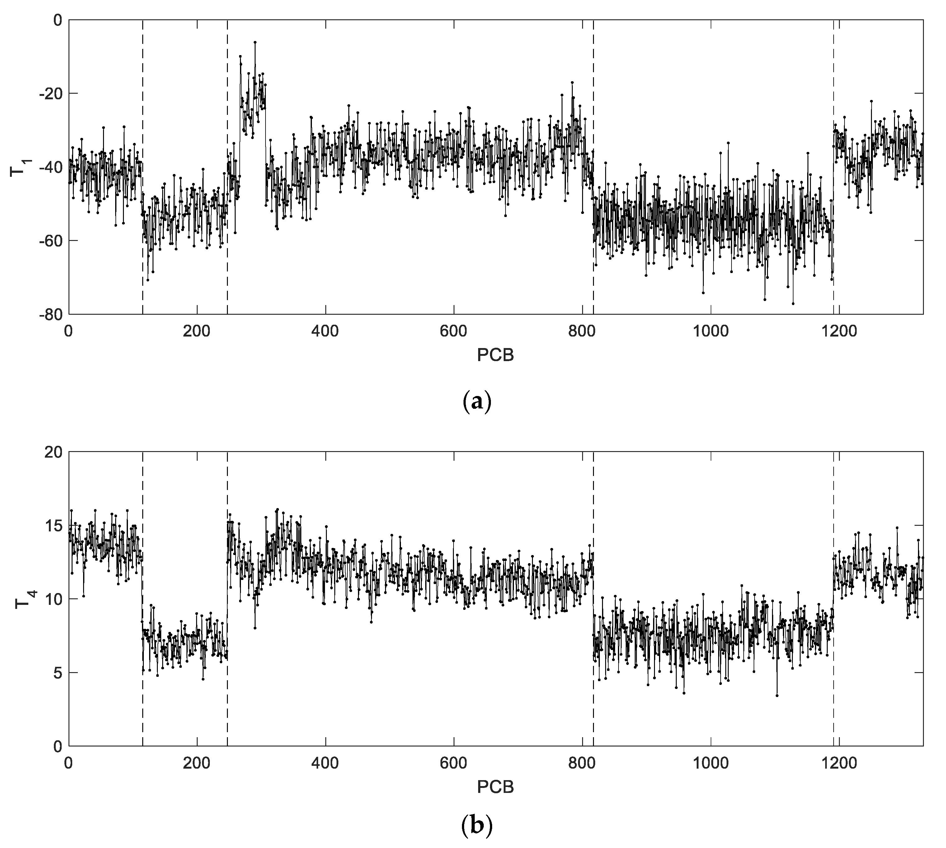
This dataset comprises at least six distinct operation periods (
Figure 16). Once again, these periods are mostly identified by PC1 and PC4, meaning that they are related to lots with different characteristic rotations in the PCBs during the SPD printing process. This result also highlights that the rotation effects on the offsets is mostly driven by inter-lot variation. From
Figure 17 it is also verified that the selected values for the tuning parameters of the AGV module led to simulated lots resembling real data.
Although the AGV module generates data with realistic features, the PCA-based monitoring methodology presents limitations in its detection capabilities due to the incorporation of inter-lot variability (
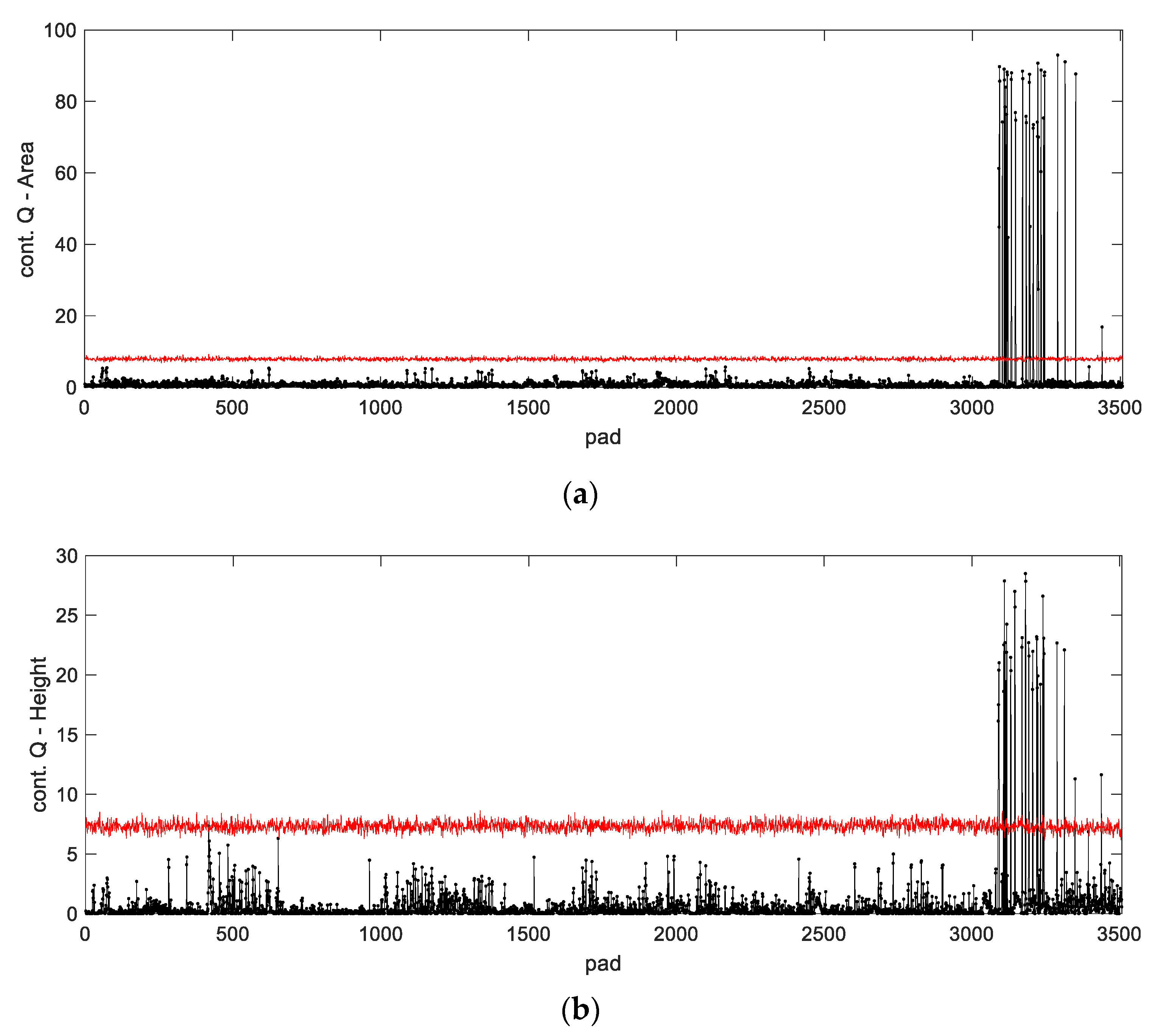
Figure 18). For instance, from the
Q-statistic, it is observed that PCBs #248, #401 and #1191 have larger deviations than the others. Nevertheless, these deviations are not large enough to overcome the sum of squared residuals over a large number of variables. By inspecting the contribution plots for these PCBs, it is verified that some of the pads have unusual heights (
Figure 19) and therefore these PCBs should have been signaled as potentially faulty. Once again, this issue may be solved in the future if the squared residuals below a given threshold are not included in the
Q-statistic, which will cause the monitoring scheme to be more sensitive to critical deviations.
6. Discussion
A suitable monitoring scheme requires an adequate model that describes the normal operations conditions of the process. One way to construct such NOC model is through the use of data-driven methods based on historical records of normal operation. However, when a new product enters the production line, such past information is not available. To overcome this situation, one can simply run the process without monitoring until sufficient data is acquired. However, this approach can lead to inadequate models since the data collected in a short period of time might not represent the overall variability of the process. This is particularly more relevant when the process has non-stationary characteristics, such as those caused by distinct production lots. As an alternative to the current data-driven modelling approaches, it is here proposed to generate artificial data based on accumulated process knowledge and then build a monitoring scheme using the augmented NOC dataset, enriched with information about inter-lot variation sources.
In this work, the proposed AGV module aims to simulate the structural components of common cause variability of a solder past printing process, accounting for (i) translation and rotation effects on offset-X and offset-Y, (ii) squeegee effects on offset-Y and height (iii) and solder mask effects on height. Furthermore, these effects are structured into multiple components in order to accommodate for inter-lot (common to all PCBs in a lot), intra-lot (common to all pads in a PCB) and pad specific (unique to each pad) variability. The amount of variability attributed to each component, as well as the magnitude of the effects is established by a set of tuning parameters handily defined by the user.
Throughout this work, it was observed that the tuning parameters can define a large variety of operation conditions. While this gives a high degree of flexibility to the AGV module, it also implies that selecting the best set of tuning parameters is a critical task in order to achieve realistic simulations. In this case, we had accesses to historical data and the tuning parameters were chosen to resemble the real data of the product under study. For a new product with distinct characteristics, the best combination of tuning parameters might be different. We expect the tuning parameters to be related to external factors such as operators and equipment operation and therefore they should not vary much from product to product. Nevertheless, further analysis is required to confirm this conjecture and the applicability of the similar tuning parameters to PCBs with different layouts.
By use of the PCA model built on the simulated data, it was verified that the simulated data was distributed in clusters related to the simulated lots. This behavior was also observed for the real data. Real data was dispersed over the same range of values as simulated data, which confirms the reliability of the AGV module as a realistic data augmentation tool. The loadings of the PCA model trained on the simulated data also showed to be related with known phenomena of the printing process. Therefore, the PCA model can provide very useful insights on the operation conditions of each PCB, as well as fault diagnosis. For instance, the PCA model can be used to identify distinct lots and the printing direction.
In this study the number of simulated lots was selected to have a reasonable representation of the process variability while also allowing for an easy visualization of the results. For a more accurate representation of the process the number of lots should be selected as the point where the PCA parameters and control limits stabilize. Throughout this work several realizations of 20 lots were simulated, and it was confirmed that they lead to consistent results of the PCA models and control limits for the statistics.
Following the good results in terms of process modelling, the PCA model was used for process monitoring. In this regard, the monitoring scheme showed to solve the excessive false alarms problem of current methodologies, at the cost of presenting low sensitivity to fault detection when faults are located on a relatively small number of SPDs. The reason for this is twofold. Firstly, the PCA model was built to account for the variability across multiple lots. However, for a given lot, the PCBs are likely to vary within a localized region of the principal components subspace. Furthermore, to detect abnormal PCBs within a lot, their measurements must differ not only from the typical measurements on their lot, but also typical measurements on other lots. Secondly, deviations from the PCA model can be masked by the sum of squared residuals over a very large number of variables. To overcome this limitation, in analogy to the cumulative sum (CUSUM) control chart [
6,
11], we propose to screen for the relevant residuals (i.e., those above a given allowance threshold) and then build a truncated
Q-statistic using only the residuals that were found relevant. This approach is already under development and preliminary results show that it reduces the number of variables/residuals included in the
Q-statistic and therefore puts more focus on the most critical deviations.
Although none of the case studies led to alarms, fault diagnosis was run for PCBs with atypical monitoring statistics. For these cases, the contribution plots were able to identify abnormal measurements as well as the affected pads. Therefore, the resort to simulated data can provide useful information for fault diagnosis. These results also support the development of an alternative monitoring statistic to enhance the detection of deviations in the residual subspace.
Finally, it is noted that real data can also be included in the PCA model as the process progresses. Another improvement that can be made as soon as real data is available is to replace the correction constants for the volume (f, Equation (20)) by those computed from real data. Consequently, the relationships between volume and the product of area and height will be closer to reality. Nevertheless, even without the use of real data, the current study already demonstrates the usefulness of the AGV module for process monitoring when historical data is not available.
7. Conclusions
In this work, a data augmentation framework for Artificial Generation of common cause Variability in SMT industrial assembling lines was proposed. The aim of the AGV module is to allow for a prompt application of monitoring procedures in new products for which extensive historical data is not available, without incurring in prohibitive rates of false alarms. The AGV module is based on process knowledge and codifies the dominant modes of common cause variation due to known physical phenomena. The proposed approach can be even implemented in the absence of an historical dataset, as long as there is accumulated information from related processes. This particular aspect was also covered in our analysis in this paper.
The data generated by the AGV module proved to reproduce well the long term variability of real process data. The critical issue of high false alarm rates was solved. On the other hand, we also report that the monitoring statistics show limited detection capabilities. This happens because the PCA model accounts for inter-lot variation, while the process will typically operate in localized regions at a given time. Furthermore, the sensitivity of the PCA monitoring scheme is also affected by the very large number of variables under monitoring.
Future work should therefore consider the application of the AGV module to other case studies. Furthermore, novel monitoring approaches should be development in order to account for the presence of different lots (improve the sensitivity of the T2-statistic) and reduce the impact of irrelevant residuals when the number of monitored variables is very large (improve the sensitivity of the Q-statistic).


