Model-Free Extremum Seeking Control of Bioprocesses: A Review with a Worked Example

Abstract

Uncertainty is a common feature of biological systems, and model-free extremum-seeking control has proved a relevant approach to avoid the typical problems related to model-based optimization, e.g., time- and resource-consuming derivation and identification of dynamic models, and lack of robustness of optimal control. In this article, a review of the past and current trends in model-free extremum seeking is proposed with an emphasis on finding optimal operating conditions of bioprocesses. This review is illustrated with a simple simulation case study which allows a comparative evaluation of a few selected methods. Finally, some experimental case studies are discussed. As usual, practice lags behind theory, but recent developments confirm the applicability of the approach at the laboratory scale and are encouraging a transfer to industrial scale.

1. Introduction

1.1. Extremum Seeking: A Real-Time Output Feedback Optimization Technique

Real-time optimization (RTO) of steady-state plants stems from computer-aided production engineering (CAPE) and aims at improving process performance through the optimization of a measurable criterion or objective function under economical, safety or quality constraints [1]. One of the most critical limitations of earlier RTO methods lies in model accuracy, and this has lead to adapted RTO techniques [2] which take possible plant–model mismatches into account. The resulting model adaptations may impact the optimization sequentially as in run-to-run methods developed by [3], or also impact the optimization criterion and the related constraint gradients which are modified to match with the true plant [4,5]. Direct input adaptation methods transforming the RTO into a feedback control problem constitute a third alternative exploiting the invariance properties of the steady-state plant. These latter methods include:

• Self-optimizing control (SOC), which tracks specific invariants or set-points of the considered process to achieve an indirect optimization [6].
• Extremum seeking control (ESC), which aims at driving the system to optimal operating conditions corresponding to the extremum of a measurable convex objective function [7,8,9].
• Necessary conditions of optimality (NCO) tracking, which uses the NCO as invariants to enforce optimality conditions [10,11,12] and gradient-based optimization. They are therefore considered the run-to-run optimization parent branches of both SOC and ESC;
• Dynamic real-time optimization (DRTO) [1,13,14], which originates from the integration of RTO strategies, achieving process operating condition updates, in a model predictive control (MPC) framework. The recent additions of economic costs and constraints has lead to the introduction of DRTO solutions in the form of nonlinear MPC strategies with economic objectives [14].

Figure 1 shows the extremum seeking control (ESC) scheme as a simple output feedback where the objective function y is assumed to be measurable and the controller drives the system to an optimum $y^{*}$ of the steady-state function $y=h\left(u\right)$.

1.2. The Origins of ESC

Before delving into the specific subject of ESC of bioprocesses, this section gives a brief historical perspective of the development of ESC in a more general context. For more details and references, we direct the reader to the excellent review of Tan [8] which covers 90 years of developments starting in the 1920s, and the recent research monograph of Scheinker and Krstic [15].

The idea of using a perturbation signal at the system input and observing its effect at the output to estimate the slope of a nonlinear static map can be traced back to the work of the French engineer Leblanc in 1922 [16] in the context of power transfer from a transmission line to a tram car. However, it seems that it was only during World War II that the technique was investigated again by Russian scientists [17]. In 1951, Draper was the first to report research on the subject in the English literature [18]. The $50s$ and $60s$ were then flourishing with various works, such as [19,20], essentially contributing to the algorithm’s performance without truly developing a systematic design framework. In this period, Blackman [21] published an interesting survey of those methods.

Basically, classical ESC methods can be subdivided into methods that involve an external perturbation (dither) signal and those which do not require one and resort to relay switches [18,22] or sliding mode techniques [23].

In 1971, a first Lyapunov stability analysis of a so-called peak-holding scheme, in which the gradient of the performance index is not estimated, but the variation of a parameter allows sensing the direction in which the performance index is evolving, was developed by Luxat and Lees [22]. Three decades were needed for a general stability analysis by Wang and Krstic [24] following the impulse of [25] in developing the framework of ES.

An important milestone in fostering the popularity of ES is the publication in 2003 of the research monograph [7] by Ariyur and Krstic.

From an (real-life) application point of view, ES was applied successfully in various fields including maximum power point tracking in photovoltaic systems [26,27], drag reduction in formation flight [28], continuously variable transmission [29], ignition systems in combustion engines [30], vapor compression systems [31,32], wind energy conversion systems [33], cavity resonators [34,35], braking sytems in automotive industry [36].

The classical perturbation-based ES scheme suffers from the time-scale separation between the process which is considered as “fast” (as the process has to settle down quickly and be viewed almost as a static map by the controller), and the perturbation signal which must be slow with respect to the process dynamics. Successful applications mostly consider relatively fast electrical and mechanical systems where the slow convergence of ES is not detrimental. Applications with large time constants and long transient phases are more problematic, as is the case for bioprocesses which are the subject of the next sections. One way around the slow convergence is to include some prior knowledge about the model, leading to model-based ES, or some form of parameter estimation, which allows one to keep on model-free extremum seeking. This distinction is also addressed in the following.

1.3. ESC of Bioprocesses

The classical bioprocess optimization problem [37,38] considers a culture of microorganisms or cells in a continuous bioreactor where the following generic reaction takes place

$$k_{1}S\to X+k_{2}P$$

(1)

where X, S, and P denote, respectively, the biomass (microorganism/cell population), the limiting substrate, and the product of interest. $k_1$ and $k_2$ are stoichiometric coefficients. The reaction kinetics can be described by various laws, among which the most popular are Monod law (2a) describing substrate activation; Contois law (2b) describing substrate activation and biomass inihibition; and Haldane law (2c), describing substrate activation at low concentrations, and inhibition at higher concentrations:

$$\begin{array}{}\mathrm{(2a)}& {\mu }_M& =\frac{{\mu }_{max}s}{K_s+s}\mathrm{(2b)}& {\mu }_C& =\frac{{\mu }_{max}s}{K_{c}x+s}\mathrm{(2c)}& {\mu }_H& =\frac{{\mu }_{max}s}{K_s+s+\frac{s^2}{K_I}}\end{array}$$

Mass balances lead to a set of ordinary differential equations:

$$\begin{array}{}\mathrm{(3a)}& \dot{x}& =\mu x-Dx\mathrm{(3b)}& \dot{s}& =-k_1\mu x-D(s-s_{in})\mathrm{(3c)}& \dot{p}& =k_2\mu x-Dp\end{array}$$

The measurable (via direct measurements or state estimation) performance index can be linked to the productivity of the biomass, the product of interest, or the reaction rate:

$$\begin{array}{}\mathrm{(4a)}& y_x& =Dx\mathrm{(4b)}& y_p& =Dp\mathrm{(4c)}& y_{\mu }& =k_2\mu x\end{array}$$

Optimization of bioprocesses was first addressed in 1999 by [37] in a numerical study using a classical ES scheme with a sinusoidal dither signal and a combination of high-pass and low-pass filters (further developed in [7]). In the same period, the experimental work of Akesson [39,40] applied a simple and practical probing method in the spirit of the peak-holding algorithm of Luxat and Lees [22], the idea being to send pulses of substrate and sense whether it is consumed by the micro-organisms. This work can be considered as the seed of a more general ES theory using nonlinear programming and developed in [41].

2. Extremum Seeking Approaches

Depending on the available knowledge about the model structure, different extremum seeking approaches have been developed. Logically, the better the system is known, the more efficient the controller may be. Roughly, the ES controllers can be classified into two main streams:

• Model-based strategies, wherein a model-based controller takes advantage of the knowledge about the model structure and either estimates the unknown parameters from online information, or exploits some robustness properties.
• Model-free strategies, wherein online information is directly exploited to estimate the gradient of the measurable cost function, and to drive the process to the optimum using feedback control. No prior knowledge about the kinetic model is required, and the optimum is simply reached by driving the process wherein the estimated cost function gradient vanishes.

Of course, the two streams are not strictly disjunct, and for instance, one can imagine taking advantage of any prior knowledge to improve a model-free strategy. While this paper mostly focuses on the second category of methods, the first stream has brought a number of important results that are briefly reviewed in the next section.

2.1. Model-Based Strategies: Uncertain Trajectory Tracking

Model-based ES strategies rely on a hypothetical kinetic structure and aim at driving the system to an optimal operating point or along an optimal operating trajectory. Since kinetic parameters are unknown or at least uncertain, the control law requires their estimation by adaptive laws or the consideration of model uncertainties and robust design.

2.1.1. Adaptive Output Feedback Control

The concept of adaptive ESC of nonlinear systems with uncertain parameters has been developed by Guay and Zhang [42], who introduced an “inverse optimal” approach to solve the optimization problem. The application of this method to continuous bioreactors has been proposed in the wake of this latter publication in [43] starting from the simple microbial growth model (3a), (3b), and (4c). These equations can be rewritten in the following compact form, replacing the kinetic term by its measurement:

$$\begin{array}{}\mathrm{(5a)}& \dot{x}& =\frac{1}{k_2}y-Dx\mathrm{(5b)}& \dot{s}& =-\frac{k_1}{k_2}y-D(s-s_{in})\end{array}$$

Define the dilution rate as the system input ($u=D$); then an extremum seeking control law is proposed to drive and stabilize the system in the neighborhood of $y^{*}=f\left({\mu }^{*}\right)$. Analyze the behavior of the output time derivative $\dot{y}=h(x,s,u,\theta )$ where $\theta$ contains the stoichiometric parameters $k_1$ and $k_2$ but also the kinetic parameters involved in the hypothetical structure of $\mu$. Since these parameters are unknown, parametric adaptive laws are inferred from the overall loop, including the extremum search combined with the adaptive controller. Stability and convergence studies resort to Lyapunov stability theory coupled to LaSalle–Yoshizawa’s theorem, LaSalle’s invariance principle, or Barbalat’s Lemma [44,45,46]. Further application results can be found in [38,47], which propose model-based extremum seeking controllers optimizing either the reaction rates or the biomass production of continuous and fed-batch processes, characterized by substrate activation and saturation following Monod kinetics (2a). Further, Refs [48,49,50,51] have extended these studies to Haldane kinetics (2c), which represents the additional effect of substrate inhibition at high concentrations. More complex kinetic structures have been considered in [52] where biomass productivity is optimized under the assumption of microbial overflow metabolism [53]. In this case, growth inhibition results from the accumulation of by-products reducing the cell respiratory capacity, and the kinetics involve switching between different models. As discussed in the survey [47], adaptive extremum seeking can be generalized to the situations where no prior knowledge is assumed, using universal approximators such as neural networks [54].

2.1.2. Sliding-Mode Control

Another approach consists of optimizing the cost function by sliding-mode control along the cost function manifold and choosing its gradient as switching function $\sigma =\frac{\partial y}{\partial u}$. Based on this idea, Lara-Cisneros et al. [55] proposed the optimization of fed-batch bioreactors modeled by (3) using a sliding-mode extremum seeking control combined with a high-gain observer estimating the uncertain kinetics. This study was extended to a two-stage anaerobic digestion model in [56]. In the same spirit, Vargas et al. [57] tackle the problem of biomass productivity optimization in bacteria cultures, presenting overflow metabolism using a two-level controller with super-twisting observers as process output estimators. Further, an input-output linearizing sliding-mode control is derived for well-defined relative degree systems with minimum phase in [58,59].

2.1.3. Integration of ES to Model Predictive Control

The optimization problems introduced in Section 2.1.1 and Section 2.1.2 do not consider constraints, which can be unrealistic in the context of real-life applications. Indeed, industrial processes are run under specific conditions implying media compositions, mininum and maximum authorized production rates, and energy consumption costs. Application of ES control to constrained optimization problems of control-affine nonlinear systems such as (3) was first proposed in [60] using a flatness-based approach. The optimal trajectory is generated by adaptive ES, and a state and input-constrained dynamic nonlinear programming problem is solved using an interior-point technique. This approach is applied to batch processes in [61].

The study of [13] generalizes the approach by integrating ES to model predictive control (MPC) considering a time-varying economic cost function based on a model presenting parametric uncertainty sets and state constraints. Uncertainty issues are solved by considering min-max optimization to determine the worst/best solutions with respect to the parameter uncertainty sets and a Lipschitz-based adaptive approach imposing Lipschitz bounds. This method is extended to economic model predictive control (EMPC) in [62], which does not track a specific trajectory but directly solves the time-varying economic optimization problem.

2.2. Model-Free Extremum Seeking Control

Model-free ES strategies rely on the existence of a measurable and convex objective function but do not require prior knowledge about the process model. Their principle is to estimate the gradient of the objective function and to force this estimate to zero (a vanishing gradient being the first necessary condition for an extremum of a differentiable function).

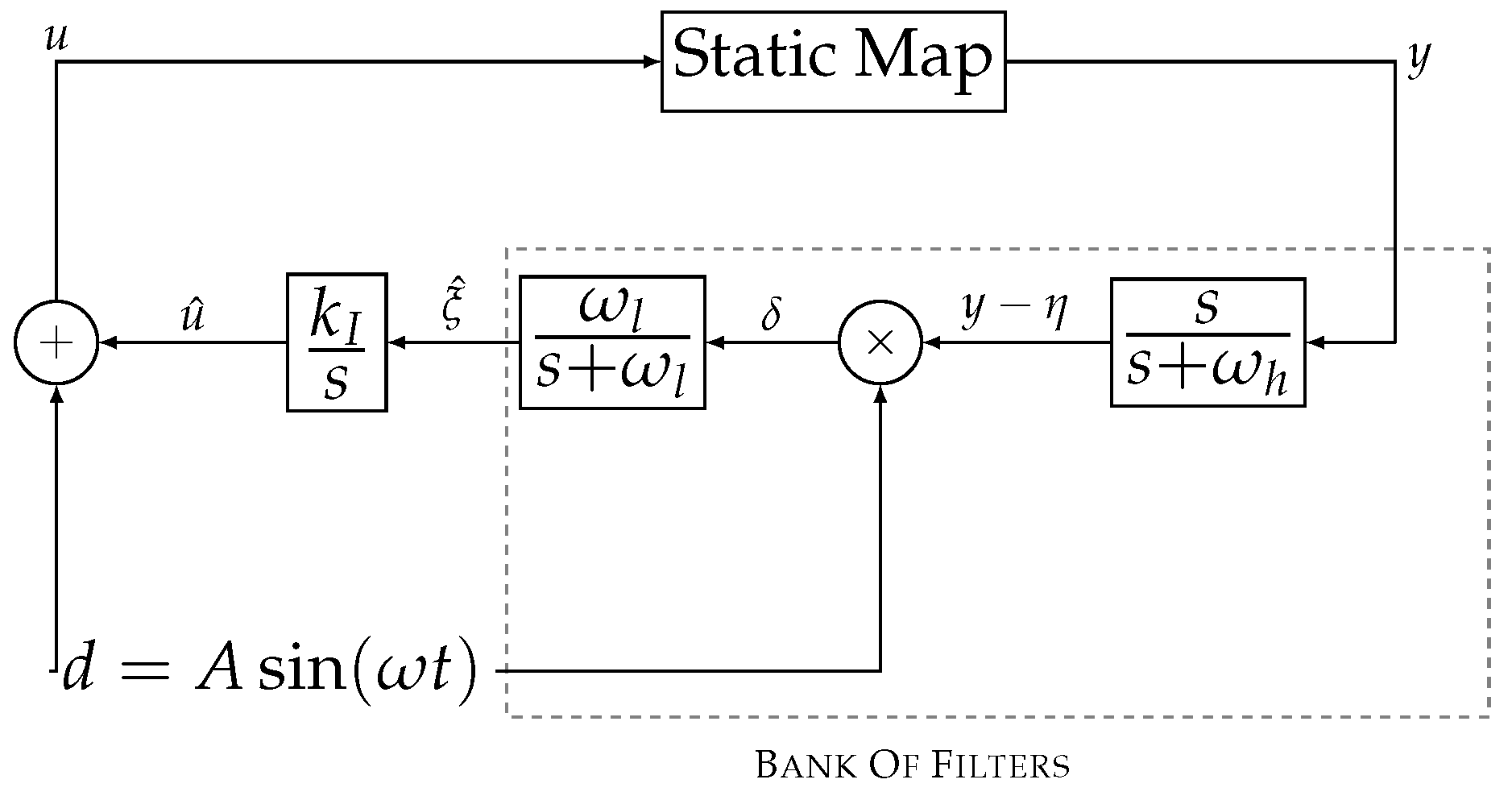
2.2.1. The Classical Pertubation-Based ES and the Use of a Filter Bank

One of the earlier forms of model-free ES is the perturbation-based ES of [7] shown in Figure 2 and described by the following equations:

$$\begin{array}{}\mathrm{(6a)}& y& =f(\widehat{u}+Asin\left(\omega t\right))\mathrm{(6b)}& \dot{\widehat{u}}& =k_I\xi \mathrm{(6c)}& \dot{\xi }& =(y-\eta )Asin\left(\omega t\right)\mathrm{(6d)}& \dot{\eta }& =-{\omega }_h\eta +{\omega }_{h}y\end{array}$$

where $\widehat{u}$ is the estimated input; $u=\widehat{u}+d$ stands for the input signal applied to the process, including a sinusoidal dither signal $d=Asin\left(\omega t\right)$; y is the measurable objective function; $y-\eta$ is the high-pass filtered output, that is, without a continuous component; $\delta$ is the demodulated signal resulting from the multiplication of $y-\eta$ by d; and $\widehat{\xi }\approx \frac{1}{k_I}\frac{\partial \widehat{u}}{\partial t}$ is the gradient estimation, obtained as the output of an optional low-pass filter. The use of a bank of filters leads us to designate this scheme as “BOF” (a wink to the French speaking reader, but there is no prejudice in this denomination) in the sequel of this review (see Figure 2).

The design parameters of this ESC have to obey some rules: the cut-off pulsations of the low-pass filter ${\omega }_l$ and high-pass filter ${\omega }_h$ should be smaller than the dither signal pulsation $\omega$; i.e., they should be located in the interval $\left]0\omega \right[$. On the other hand, the dither signal pulsation $\omega$ should be small with respect to the process dynamics—for the process to be in periodic steady state—and its magnitude sufficiently large to overcome the information attenuation by the filters.

These rules reflect the time-scale separation [7] already highlighted in the introduction to this review, where:

• The process has the fastest dynamics, which, in the limit, can be seen as a static map;
• The dither signal has intermediate dynamics;
• The gradient estimator has the slowest dynamics.

It is important to note that the issue of the time-scale separation worsens in cases of systems with multiple inputs [7]. In the particular case of multi-input single-output systems with r inputs, it is necessary to design $\frac{r+2}{2}$ (rounded to the next lower integer) dither frequencies [63], thereby requiring more time separations and slowing down the gradient estimator.

A suitable choice of the design parameters ensures an exponential convergence of y in a $O(\omega +A)$ neighborhood of the optimum $y^{*}=f\left(u^{*}\right)$ [64], where $u^{*}$ is the corresponding optimum input.

Optimizing control of bioreactors using BOF-ES was first reported in [37], where a bifurcation analysis of model (3) with Monod and Haldane kinetics was achieved. This study highlights the operational limits and suggests the use of wash-out filters to guarantee the system’s stability. Subsequently, Nguang and Chen [65] proposed an illustrative application of the same strategy to continuous fermentation processes and [66] to anaerobic digestion.

However, perturbation-based techniques and the BOF-ESC are only successful if the system can be seen as almost static, that is, slowly perturbed by the dither signal. The slow convergence resulting from this time scale separation can be a serious drawback in biological applications where the dominant time constants can be very large. Moreover, the characterization of the effects of the dither signal frequency and magnitude on the convergence, as presented in [64], is a significant additional issue for general nonlinear systems. This has motivated further studies, such as [67], which concluded that the convergence accuracy of BOF-ES is only concerned with the magnitude of the dither signal for a specific class of nonlinear systems represented by Wiener and Hammerstein block-oriented models. Furthermore, Tan et al. [68] considered several dither signals and discussed their impacts on the domains of attraction, convergence, speed, and accuracy.

To alleviate the undesirable time scale separation effect, Krstic [69] suggested introducing controllers to speed-up the closed-loop dynamics or to compensate for the phase-shift introduced by the system dynamics at the perturbation frequency. This latter idea has been proven achievable by [70], depending on the system relative degree, and thus, for a restricted class of nonlinear systems.

In the last decade, several practical design guidelines have been proposed to improve the convergence rate, without true analysis, based on the selection of the operating conditions [71], or the use of several dither signals to enrich the frequency content [72,73]. In [74], an application of BOF-ESC to yeast fed-batch cultures with overflow metabolism is presented, where the convergence speed was enhanced thanks to an appropriate manipulation of the substrates presenting fast dynamics.

The first experimental validation of BOF-ES in the field of bioprocess optimization can be attributed to [75] optimizing microalgae growth at pre-industrial scale by manipulating the pH. Overall, BOF-ES can definitely be considered as a useful, practical, and easy-to-implement solution to optimize bioprocesses as long as operating conditions, dithers and controlled variables are carefully selected with respect to system dynamics.

2.2.2. Recursive Parameter Estimators

A simple solution to improve the convergence speed of perturbation-based ES algorithms is to replace the bank of filters, that is, one part of the time scale separation, in a recursive estimator as shown in Figure 3, where:

$$\begin{array}{}\mathrm{(7a)}& \hfill u& =\widehat{u}+d\hfill \mathrm{(7b)}& \hfill \dot{\widehat{u}}& =k_I\widehat{\frac{\partial y}{\partial u}}(y,u)\hfill \end{array}$$

This ES structure convergence is now only dependent on the system dynamics and the dither signal parameter selection. An illustration of this recursive strategy, using a continuous recursive least-squares (RLS) algorithm with forgetting factor [25,76], can be found in [74], which discusses the application of BOF-ES and RLS-ES to biomass productivity optimization in fed-batch cultures. The main conclusion of this study is that the recursive estimator provides a more robust behavior and a faster convergence. The continuous ES-RLS scheme is described as follows:

$$\begin{array}{}\mathrm{(8a)}& \hfill e& =y-\widehat{\xi }{\Phi }^T\hfill \mathrm{(8b)}& \hfill \dot{\widehat{\xi }}& =K{R}^{-1}{\Phi }^{T}e\hfill \mathrm{(8c)}& \hfill \dot{R}& =K({\Phi }^T\Phi -\lambda R)\hfill \mathrm{(8d)}& \hfill \dot{\widehat{u}}& =k_I\widehat{\xi }\hfill \mathrm{(8e)}& \hfill u& =\widehat{u}+d\hfill \end{array}$$

where K is the positive adaptation gain; R is the inverse covariance matrix acting as a directional adaptation gain; $\lambda$ is the forgetting factor used in order to avoid covariance wind-up issues due to the absence of bounds in R growth (if $\lambda =0$, $\dot{R}\ge 0$ [76]).

Later, Chioua et al. [77] characterized the convergence rate and proved the stability of the ES loop with RLS as the gradient estimator for nonlinear systems, independently of their possible decompositions in block-oriented models (Wiener/Hammerstein).

In the same time period, Guay and Dochain [78] have reformulated the ES description as a time-varying control problem for general nonlinear systems, using the combination of a continuous parameter estimator based on a generic prediction model of the output y (not requiring a priori knowledge on the process), and an original integral control law. The main improvement of the method lies in the use of the dither signal, which, following a favorable contribution from the natural time-variation of the unknown parameter (gradient), becomes no longer necessary. Guay and Dochain [78] therefore show that the suppression of the intermediate dither dynamics is also possible, limiting the convergence speed to the process dynamics and the estimator performance.

2.2.3. Empirical ESC: Probing Control

The model-free methods presented in Section 2.2.1 and Section 2.2.2 rely on the existence of a convex and measurable objective function. When the available process instrumentation does not allow this latter condition to be verified, one may resort to more practical or even empirical software solutions. For instance, optimizing biomass productivity of cells exhibiting overflow metabolism requires one to measure an objective function related to the cell respiratory capacity which should be maximal in order to optimize substrate consumption [53]. This critical measurement can, however, only be achieved indirectly [74] and the convex objective function is reconstructed using measurement signals and some prior knowledge about the reaction stoichiometry. The performance of the ES technique therefore depends on the stoichiometric coefficient estimation accuracy, which may become critical. In the early 2000s, Akesson et al. [39] proposed an interesting empirical probing control method detecting the possible saturation of the respiratory capacity of Escherichia coli, and in turn, inhibitory by-product (acetate) accumulation [39], by measuring the oxygen uptake following a sudden change in the substrate (glucose) uptake caused by feed pulses. Indeed, when the cell’s respiratory capacity is saturated, the dissolved oxygen concentration (measured variable) does not vary any longer, since cells are not able to assimilate more oxygen. In analogy with classical ESC, probing control uses these pulse sequences as dither whose magnitude and frequency are designed in accordance with the sensitivity level of dissolved oxygen variation detections, and the combined respiratory capacity and substrate uptake maximization define the extremum of an unknown objective function. Probing control became popular during the first decade of the 21st century, promoted by several experimental studies in various fields such as human health [79] and agriculture [80].

The characterization of overflow metabolism for yeasts (S. cerevisiae, P. pastoris) and bacteria (E. coli) was also provided by [81] using probing control and a scaling-up approach of the method was proposed by [82].

3. Convergence Issues and Acceleration

The ESC problem, as defined in the previous sections, assumes basic practical constraints such as fast process dynamics (with respect to the dither and the optional filters) and a single measurable objective function. However, several issues may arise when the process natural dynamics are detrimental to objective-related time restrictions or when several competing objectives must be handled. In the following, some practical ways to manage and accelerate the ESC loop convergence are addressed, starting with a simple feedback form.

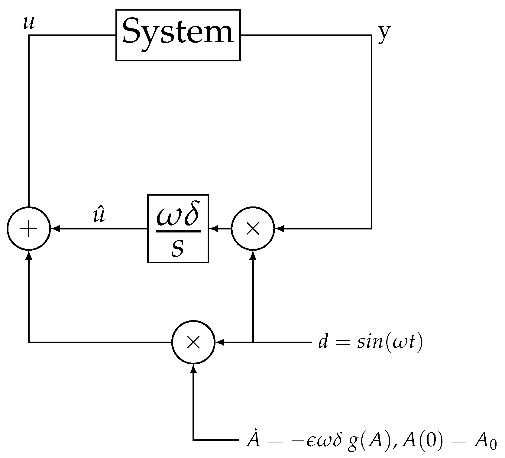
3.1. Extremum Seeking Control: A Simple Output Feedback Form

A minimal ESC loop description, as illustrated in Figure 4, considers two blocks: the gradient estimator and the integral controller pushing this gradient to a reference value (in the case of extremum seeking, zero) ${\xi }_{ref}$ such that the error $ϵ={\xi }_{ref}-\widehat{\xi }$ is zero. A simple pole-placement procedure can be used to define the ES closed-loop dynamics, i.e., to design the integral constant $k_I$. As discussed in [83], a controllable state-space representation of the gradient evolution can be inferred as:

$$\begin{array}{}\mathrm{(9a)}& \hfill \dot{\xi }& =A\xi +Bw(u_{ref},\widehat{\theta })\hfill \mathrm{(9b)}& \hfill y& =C\xi \hfill \end{array}$$

where w is a function of the input reference $u_{ref}$ and the parameter $\theta$ estimated by the recursive estimator from Figure 3, both assumed to provide the desired gradient ${\xi }_{ref}$. By comparing Figure 4 with Figure 3, we can easily infer that $A=0$, $B=1$, and $C=1$. By introducing an integral action, the system reads:

$$\begin{array}{}\mathrm{(10a)}& \hfill \left[\begin{array}{c}\dot{\xi }\\ \dot{v}\end{array}\right]& =\left[\begin{array}{cc}A& 0\\ -C& 0\end{array}\right]\left[\begin{array}{c}\xi \\ v\end{array}\right]+\left[\begin{array}{c}B\\ 0\end{array}\right]w(u_{ref},\widehat{\theta })+\left[\begin{array}{c}0\\ I\end{array}\right]r\hfill \mathrm{(10b)}& \hfill y& =\left[\begin{array}{cc}C& 0\end{array}\right]\left[\begin{array}{c}{\xi }_k\\ v_k\end{array}\right]\hfill \end{array}$$

When applying classical pole-placement procedures, the closed-loop dynamics can be specified in the time domain, yielding the integral (extremum seeking) control gain. However, it must be noticed that some unexpected transient dynamics may not be taken into account and $u_{ref}$ must therefore be chosen in accordance with the domain of attraction and stability analysis, often restricting the input operating range to a specific interval $\left[u_{min}{u}_{max}\right]$. Consequently, if the closed-loop response presents transients due to neglected system dynamics, such that the input is out of this permissible range, the overall system may fall into unstable regions. To minimize the risks of loop destabilization, a sufficient level of robustness should be imposed, with large gain margins and limited overshoots.

3.2. Proportional-Integral Extremum Seeking

In an alternative attempt to accelerate the convergence of the ESC, Guay and Dochain [84] first proposed to combine the time-varying estimation method from [78] with a proportional-integral controller, as shown in Figure 5. This method generalizes standard ESC using the integral action as “extremum seeker” and proportional action as the fast optimizer of the objective function, amplifying the estimated gradient descent or ascent effect. A general formalism of proportional-integral extremum seeking control scheme (PIESC) has been provided by the same authors in [85].

The closed-loop PIES controller reads:

$$\begin{array}{}\mathrm{(11a)}& \hfill u& =k_p\widehat{\xi }+\widehat{u}+d\hfill \mathrm{(11b)}& \hfill \dot{\widehat{u}}& =k_i\widehat{\xi }d\hfill \end{array}$$

where $k_p$ and $k_i$ are respectively the proportional and integral gains.

A second PIESC approach has also been proposed by [86], using the classical perturbation-based BOF scheme. In this study, the parameter (gradient) estimator block in Figure 5 is replaced by an output derivative $\dot{y}$ estimator modeled by a high-gain high-pass filter block with transfer function $\frac{{\omega }_{h}s}{s+{\omega }_h}$ and ${\omega }_h>>$. The filter output may then be read as:

$$\begin{array}{}\mathrm{(12a)}& \hfill \widehat{\xi }\approx \widehat{\dot{y}}& =-{\omega }_h^2\nu +{\omega }_{h}y\hfill \mathrm{(12b)}& \hfill \dot{\nu }& =-{\omega }_h\nu +y\hfill \end{array}$$

The tuning rules proposed by [86] may be summarized as follows:

• The PIESC with BOF converges to a $\frac{1}{\omega }$ neighborhood of the optimum and $\omega$ should therefore be chosen sufficiently high;
• $\nu \left(0\right)$ should be chosen equal to $\frac{y}{\omega }$ to avoid sudden initial jumps arising from $\dot{\nu }$;
• ${\omega }_h$ should be of a greater order of magnitude than $\omega$ to favor the derivative effect.

An application of the PIESC to the optimization problem of compressor discharge temperature setpoint selection for a vapor compressor system, minimizing power consumption, has recently been achieved by [87], who showed the performance of the method in realistic operating conditions (noise, input/sensor quantization), through experimental validation on a room air conditioner. As a result, the PIESC is able to achieve the optimizing control in a time-scale in the order of the process dynamics. Since no PIESC design for bioprocesses has been made available in the literature, a first attempt is provided in the current review in Section 4.1 and numerical results are in Section 4.4.

3.3. Dynamic Modeling with Block-Oriented Representations

As stated in Section 2.2.1 and Section 2.2.2, the convergence accuracy of BOF-ES and RLS-ES applied to a specific class of nonlinear systems represented by Wiener/Hammerstein (W/H) block-oriented models, is only impacted by the dither signal magnitude. Semi-global stability results of the application of observer-based extremum seeking to W/H plants is presented as an extension of the work of [88] in [89,90], showing that the ES scheme requires the knowledge of the relative orders of both input and output dynamics of the plant. From the latter results, a discrete version of the method for W/H plants with knowledge limited to the linear dynamics is also proposed, suggesting guidelines for the choice of the ES parameters, first setting the dither signal magnitude and then adapting the ES integral gain. The latter also presents an experimental validation of the method on a spark-ignition engine. Eventually, the same authors proposed directly adding some model knowledge in the adaptation scheme of the fast extremum seeking method in [91]. Interestingly, this allows improving convergence not by completely removing the time-scale separations of, in decreasing speed order, the optimizer and the estimator, but by reversing them, that is, by accelerating the estimation and subsequently the optimization. Another fast algorithm using proportional-integral phasor extremum seeking was proposed by [92] for W/H systems; its semi-global and practically asymptotical stability was shown. The principle is to drive the system to its optimum by considering the measured output phasor, from which a proportional approximation of the static cost function gradient is obtained, under the assumption of a priori known input and output dynamic block relative orders. It should be noticed that considering the phasor allows taking both the gradient and the phase shift, respectively related to the static map and the plant dynamics, into account. This estimator is then combined to a PI-ES scheme, in the spirit of [86] with an original amplitude update mechanism reducing the perturbation amplitude as the algorithm approaches the optimum vicinity, in the spirit of [93], which will be discussed in the next subsection.

In the field of biosystems, Feudjio et al. [83] proposed an advanced auxiliary model-recursive prediction error method (AM-RPEM)-based ES algorithm for systems represented by block-oriented models. In this algorithm’s structure, represented in Figure 6, a slope generator is coupled to the controller to reach any steady-state belonging to the static map, making ES a particular case of the slope-seeking strategy.

The considered class of bioprocesses is characterized by the following assumptions:

• The bioprocess is operated in continuous mode with a constant volume (the inflow is equal to the outflow);
• The measurable performance index is the biomass production $y=DX$, i.e., the product of the dilution rate D imposed by the inflow and outflow pumps by the biomass concentration X;
• The bioprocess can be approximated by a Hammerstein model [94] presenting a quadratic static nonlinearity of the form:

  $$v=M_1{u}^2+M_{2}u+M_3$$

  (13)

  where $u=D$ and v represent the static map input and output signals, respectively. This representation assumes that the performance index can be approximated, at least locally, by a quadratic form. For a maximum, it is required that $M_1<0$. The Hammerstein model also includes dynamics, which can be described by a transfer function.
• A discrete second-order transfer function may suffice to represent these dynamics:

  $$G\left(z^{-1}\right)=K\frac{(z^{-1}-\alpha z^{-2})}{1+{\beta }_1{z}^{-1}+{\beta }_2{z}^{-2}}$$

  (14)

  where $z^{-1}$ is the backward shift operator such that $z^{-1}y\left(k\right)=y(k-1)$ and K is a gain which can be chosen so as to ensure unitary steady-state gain, i.e., $G\left(1\right)=1$, which implies $K=\frac{1+{\beta }_1+{\beta }_2}{1-\alpha }$. The two poles defined by the parameters ${\beta }_1$ and ${\beta }_2$ represent the actuator and process dynamics.

Under these assumptions, the unknown model parameters can be estimated using a simple recursive least-squares (RLS) method, as originally proposed in [74], or in order to improve the convergence and precision of the estimates, the recursive prediction error method (RPEM) from [95,96], where, unlike classical RLS algorithms which provide as estimates the linear combinations of the unknown parameters, the Hammerstein model parameters are directly inferred. However, since analytically computing parametric sensitivities can be tedious, an auxiliary model is used to simplify the evaluation of the sensitivities. Another option is also provided, considering an output-error auto-regressive model [97] which is mostly useful in the presence of relatively large process/measurement noise.

3.4. Multivalued Cost Functions and Competing Objectives

An intrinsic property of the previously discussed systems is the existence of a sole extremum. For complex (bio)processes, it is legitimate to consider possible multiple local extrema of the steady-state objective function. In [93], this problem is tackled using an adaptive dither magnitude update law, specifying the conditions of convergence to the global extremum. The proposed solution consists of designing and initializing the dither signal magnitude law to allow the bifurcation towards the submap of the objective function where the global extremum is located. Since ES convergence is affected by the dither signal magnitude, the latter is adaptively decreased with time, as the algorithm approaches the global extremum. Starting from a simplified ES scheme drawn in Figure 7, the closed-loop representation can be written, denoting $\sigma =\omega t$:

$$\begin{array}{}\mathrm{(15a)}& \hfill \omega \frac{dx}{d\sigma }& =f\left(x,u\right)\hfill \mathrm{(15b)}& \hfill \frac{d\widehat{u}}{d\sigma }& =\delta h\left(x\right)sin\left(\sigma \right)\hfill \mathrm{(15c)}& \hfill \frac{dA}{d\sigma }& =-ϵ\delta g\left(A\right)\hfill \end{array}$$

where f stands for the nonlinear state space function of the system, x is the state vector, $\delta$ is a positive design parameter, $A\left(t\right)$ is the varying magnitude of the dither signal with $A\left(0\right)>0$, and $g\left(A\right)$ is a locally Lipschitz function that is zero at zero and positive otherwise. Fast and slow dynamics are inferred by considering x in equilibrium, that is, $x_{eq}=l(\widehat{u}+Asin\left(\sigma \right))$, which is assumed to be asymptotically stable, leading to the following reduced system:

$$\begin{array}{}\mathrm{(16a)}& \hfill \frac{du}{d\sigma }& =\delta h\circ l(u+Asin(\sigma \left)\right)sin\left(\sigma \right)=\delta Q(\sigma ,u,A)\hfill \mathrm{(16b)}& \hfill \frac{dA}{d\sigma }& =-ϵ\delta g\left(A\right)\hfill \end{array}$$

Considering the corresponding average system over one $2\pi$ period and introducing $\tau =ϵ\delta \sigma$, (16) becomes:

$$\begin{array}{}\mathrm{(17a)}& \hfill ϵ\frac{du}{d\tau }& =Q_{av}(\sigma ,u,A)\hfill \mathrm{(17b)}& \hfill \frac{dA}{d\tau }& =-g\left(A\right)\hfill \end{array}$$

Tan et al. [93] have shown that there exists a continuous function $p(u,A)$ such that $Q_{av}=Ap(u,A)$. The standard singular perturbation technique is unfortunately not applicable (for more details about this statement, see [93]) and it is therefore recommended to analyze the convergence properties of the ES scheme for a specific initialization $A\left(0\right)=A_0$, assuming that there exists an isolated and unique real solution $u=\ell \left(A\right)$ to $Q_{av}=0$ such that ℓ is continuous and $\frac{\partial p}{\partial \ell }<0$ for all $A\ge 0$ and $u^{*}=\ell \left(0\right)$ is the global optimum. Following this latter assumption, it may be demonstrated that the convergence of the extremum seeking scheme of Figure 7 to $u^{*}$ is practically semi-global. The global extremum of a multimodal objective function can therefore be reached by the perturbation-based ES following judicious choices of the initial dither signal magnitude and the function $g\left(A\right)$.

A practical interpretation of the latter results in optimal operating mode seeking for bioprocesses is discussed in [98], where a multivalued cost function originating from the combination of both yield and production objective functions is derived from model (3) where only the biomass and the substrate are considered. The kinetics are modeled by a simple Monod law and an exponential factor representing growth inhibition by the substrate (which, physically, can be compared to the Haldane kinetics (2c)). Consequently, the resulting cost functions present two distinct quasi-steady-state maps between which the ES algorithm must be able to operate a switch when initialized on the map which does not contain the global extremum. Considering only the stable branch, the set-valued cost function $Q(u,A)$ is, in this particular case, defined as a set of two continuous single-valued functions such that, omitting u and A for the sake of clarity, $Q=\left\{Q_1,Q_2\right\}$ with the conditions:

• $Q_1$ is defined on $[u_1,+\infty [$ and $Q_2$ on $]-\infty ,u_2]$ with $u_1<u_2$;
• For each value of $u_1$ and $u_2$, there are asymptotically stable equilibria $x={\ell }_1\left(u_1\right)$ and $x={\ell }_2\left(u_2\right)$;
• $Q_2>Q_1$ for all u;
• $Q_1^{\prime }<0$;
• $Q_2$ has a unique global maximum in $u_1<u^{*}<u_2$.

To enable some switch conditions from one single-valued cost to the other, in addition to the application of the results from [93], it is concluded that restrictive conditions involving the initial value $A_0$ and $g(u,A)$ should be used in order to make the strategy successful, also implying a loss of performance.

The existence of several extrema may also result from a dynamic separation interpretation. Even if a process presents a single and a priori global optimum on the steady-state map, the isolated fast dynamic analysis may reveal the existence of a transient extremum. An illustration based on the CANON process, used to remove ammonium from concentrated wastewater streams, is provided by [99] where the fast dynamics, called the boundary layer model, are represented by the substrate and flow dynamics, while biomass growth is assumed to be the slow dynamics. In this example, even when the biomass is not at steady-state, there exists a transient optimum on the boundary layer, and more interestingly, it turns out that locally optimizing the transient objective leads to the global optimization of the steady-state objective function, which comes to optimize an instantaneous objective without taking the future trajectory into account. A phasor-based extremum seeking controller inspired by [100] is therefore applied and the resulting algorithm is called “greedy” ES in analogy to greedy algorithms in computer science [101] that select the best instantaneous options without regard to future decisions.

4. An Illustrative Example: Optimization of Biomass Productivity

The aim of this section is to provide a worked illustrative example of the respective performances of the model-free ES algorithms introduced in Section 2.2 and Section 3 where biomass production (4a) is optimized using model (3) and considering three classical kinetic structures: Monod (2a), Haldane (2c), and Contois (2b) laws. All the parameter values used in the following simulations are included in

Table 1. Parameter values of model (3) considering Monod, Haldane or Contois kinetic laws.

$\mathit{Parameter}$	$\mathit{Value}$	$\mathit{Unit}$
$k_1$	0.5	$[gs/gx]$
${\mu }_{max}$	1.4	$\left[h^{-1}\right]$
$K_s$	5	$[g/L]$
$K_I$	25	$[g/L]$
$K_c$	3	$[gs/gx]$
$S_{in}$	50	$[g/L]$

.

Regarding the bifurcation analysis of system (3) with Monod and Haldane kinetics, the reader may refer to [37] for detailed results which can be summarized as follows (the wash-out equilibrium $(x_e,s_e)=(0,S_{in})$ is not considered):

$$\begin{array}{}\mathrm{(18a)}& \hfill x_e& =\frac{s_{in}({\mu }_{max}-D_e)-K_s{D}_e}{k_1({\mu }_{max}-D_e)}\hfill \mathrm{(18b)}& \hfill s_e& =\frac{D_e{K}_s}{{\mu }_{max}-D_e}\hfill \mathrm{(18c)}& \hfill D_e& <\frac{S_{in}}{k_1{K}_s}\hfill \mathrm{(18d)}& \hfill D_e^{*}& ={\mu }_{max}\left(1-\sqrt{\frac{1-S_{in}}{S_{in}+K_s}}\right)\hfill \mathrm{(18e)}& \hfill y^{*}& =D_e^{*}{x}_e\left(D_e^{*}\right)\hfill \end{array}$$

under the assumption of Monod kinetics, wherein the “e” index denotes equilibrium values and “*” index values at optimum, and

$$\begin{array}{}\mathrm{(19a)}& \hfill x_{e_{1,2}}& =\frac{S_{in}-s_{e_{1,2}}}{k_1}\hfill \mathrm{(19b)}& \hfill s_{e_{1,2}}& =\frac{({\mu }_{max}-D_e)\pm \sqrt{{(D_e-{\mu }_{max})}^2-\frac{4K_s{D}_e^2}{K_I}}}{\frac{2D_e}{K_I}}\hfill \mathrm{(19c)}& \hfill D_e& <\frac{{\mu }_{max}}{1+2\sqrt{\frac{K_s}{K_I}}}\hfill \mathrm{(19d)}& \hfill D_e^{*}& =\frac{-b-\sqrt{b^2-4ac}}{2a}\hfill \mathrm{(19e)}& \hfill a& =\left(1-4\frac{K_s}{K_I}\right)\left({(2S_{in}+K_I)}^2\right)-K_I^2-16K_s^2+8K_s{K}_I\hfill \mathrm{(19f)}& \hfill b& =2{\mu }_{max}(K_I^2-{(2S_{in}+K_I)}^2)-8{\mu }_{max}{K}_s{K}_I\hfill \mathrm{(19g)}& \hfill c& =({(2S_{in}+K_I)}^2-K_I^2){\mu }_{max}^2\hfill \mathrm{(19h)}& \hfill y^{*}& =D_e^{*}{x}_e\left(D_e^{*}\right)\hfill \end{array}$$

under the assumption of Haldane kinetics for which there exist two equilibrium trajectories.

A similar analysis using the Contois kinetic law (2b) can be achieved and provides the following original results. The new equilibrium reads:

$$\begin{array}{}\mathrm{(20a)}& \hfill x_e& =\frac{S_{in}({\mu }_{max}-D_e)}{k_1({\mu }_{max}-D_e)+D_e{K}_c}\hfill \mathrm{(20b)}& \hfill s_e& =\frac{D_e{S}_{in}{K}_c}{k_1({\mu }_{max}-D_e)+D_e{K}_c}\hfill \end{array}$$

and the equilibrium definition condition is $D_e<{\mu }_{max}$. The steady-state extremum $y_e^{*}$ can be calculated considering $\frac{\partial y_e}{\partial D_e}=0$, which leads to the following optimal dilution rate:

$$D_e^{*}=\frac{{\mu }_{max}}{1+\sqrt{\frac{K_c}{k_1}}}$$

(21)

The stability analysis of the equilibrium requires one to determine the Jacobian of system (3) while considering the Contois kinetic law, which yields:

$$\begin{array}{}\mathrm{(22a)}& \hfill Jac& =\left[\begin{array}{cc}\frac{\partial \dot{x}}{\partial x}& \frac{\partial \dot{x}}{\partial s}\\ \frac{\partial \dot{s}}{\partial x}& \frac{\partial \dot{s}}{\partial s}\end{array}\right]\hfill \mathrm{(22b)}& \hfill & =\left[\begin{array}{cc}\frac{{\mu }_{max}{s}^2}{{(K_{c}x+s)}^2}-D& \frac{{\mu }_{max}{K}_c{x}^2}{{(K_{c}x+s)}^2}\\ \frac{k_1{\mu }_{max}{s}^2}{{(K_{c}x+s)}^2}& \frac{k_1{\mu }_{max}{K}_c{x}^2}{{(K_{c}x+s)}^2}-D\end{array}\right]\hfill \end{array}$$

and in steady-state, we obtain:

$$\begin{array}{}\mathrm{(23a)}& \hfill Ja{c}_e& =\left[\begin{array}{cc}{\left.\frac{\partial \dot{x}}{\partial x}\right|}_{x=x_e,s=s_e,D=D_e}& {\left.\frac{\partial \dot{x}}{\partial s}\right|}_{x=x_e,s=s_e,D=D_e}\\ {\left.\frac{\partial \dot{s}}{\partial x}\right|}_{x=x_e,s=s_e,D=D_e}& {\left.\frac{\partial \dot{s}}{\partial s}\right|}_{x=x_e,s=s_e,D=D_e}\end{array}\right]\hfill \mathrm{(23b)}& \hfill & =\left[\begin{array}{cc}\frac{D_e^2}{{\mu }_{max}}-D_e& \frac{{({\mu }_{max}-D_e)}^2}{K_c^2{\mu }_{max}}\\ \frac{k_1{D}_e^2}{{\mu }_{max}}& \frac{k_1{({\mu }_{max}-D_e)}^2}{K_c^2{\mu }_{max}}-D_e\end{array}\right]\hfill \end{array}$$

The eigenvalues of (23) are:

$$\begin{array}{}\mathrm{(24a)}& \hfill {\lambda }_1& =-D_e\hfill \mathrm{(24b)}& \hfill {\lambda }_2& =-D_e+\frac{D_e^2}{{\mu }_{max}}+\frac{k_1{({\mu }_{max}-D_e)}^2}{K_c^2{\mu }_{max}}\hfill \end{array}$$

and the stability conditions on $D_e$ are then:

$$\frac{{\mu }_{max}}{1+\frac{K_c^2}{k_1}}<D_e<{\mu }_{max}$$

(25)

4.1. Bank of Filters with PI Control

A PIESC with BOF tuning is suggested, based on [86], as follows:

$$\begin{array}{}\mathrm{(26a)}& \hfill u& =k_p\dot{y}+\widehat{u}+d\hfill \mathrm{(26b)}& \hfill \dot{\widehat{u}}& =k_i\dot{y}d\hfill \end{array}$$

where $d=Asin\left(\omega t\right)$ is the dither signal and the output derivative $\dot{y}$ is computed by an additional high-pass filter (12), of the form:

$$\begin{array}{}\mathrm{(27a)}& \hfill \dot{\eta }& =-{\omega }_h\eta +y\hfill \mathrm{(27b)}& \hfill \dot{y}& ={\omega }_h\dot{\eta }\hfill \end{array}$$

where $\eta$ is an intermediate variable, the image of the output derivative, and ${\omega }_h$ is the filter cut-off frequency which should be chosen to be greater than $\omega$, the dither signal angular frequency. Even if some tuning rules are proposed in [86] to design $\omega$ and ${\omega }_h$, there is unfortunately no indication concerning the tuning of $k_p$, $k_i$, and the dither signal magnitude A which must be designed by trial and error. In order to illustrate the advantages of the PI method with respect to the classical BOF-ES from [7], two parametrizations are considered in the following and are summarized in

Table 2. PIESC with BOF controller parameters.

$\mathit{Parameter}$	$\mathit{Case}1$	$\mathit{Case}2$	$\mathit{Unit}$
$\omega$	$\frac{2\pi }{50}$	$\frac{2\pi }{50}$	$\left[h^{-1}\right]$
A	0.02	0.02	$\left[h^{-1}\right]$
${\omega }_h$	0.08 $\omega$	2 $\omega$	$\left[h^{-1}\right]$
$k_p$	0	0.3
$k_i$	0.05	1

. The first case corresponds to the simple BOF-ES proportional control ($k_p=0$) strategy, for which the parameters are optimally selected by trial and error to provide the best transient behavior (fastest convergence). For an accurate analysis of the choice of the dither signal magnitude and frequency, the reader may refer to [88] for semi-global stability results and [67] for the particular cases of Wiener/Hammerstein approximations. The second case corresponds to the BOF-ES PI control application with a specific parametrization respecting the tuning rules of [78].

4.2. Recursive Least-Square Estimation with PI Control

A simple recursive least-square extremum seeking algorithm (RLS-ES) combined with the PI control structure introduced in Section 4.1 is proposed in the same spirit as [85]. The PIRLS-ES controller slightly differs from (26) which is rewritten:

$$\begin{array}{}\mathrm{(28a)}& \hfill u& =k_p\widehat{\gamma }+\widehat{u}+d\hfill \mathrm{(28b)}& \hfill \dot{\widehat{u}}& =k_i\widehat{\gamma }d\hfill \end{array}$$

where $\widehat{\gamma }$ replaces $\dot{y}$ and denotes the estimator of the cost function gradient $\frac{y}{u}$. Indeed, taking the partial derivative of $y=ux$ ($u=D$) with respect to u yields:

$$\frac{\partial y}{\partial u}=x+u\frac{\partial x}{\partial u}$$

Multiplying (29) by u, we obtain:

$$\begin{array}{}\mathrm{(29a)}& \hfill y& =u\frac{\partial y}{\partial u}-u^2\frac{\partial x}{\partial u}\hfill \mathrm{(29b)}& \hfill & =\phi {\theta }^T\hfill \end{array}$$

where $\phi =\left[u1\right]$, $\theta =\left[{\theta }_1{\theta }_2\right]=\left[\gamma -u^2\frac{\partial x}{\partial u}\right]$, and $\gamma =\frac{\partial y}{\partial u}$. It must be noticed that when reaching the extremum steady state $y^{*}$, $\gamma =0$, and from (29), $y^{*}={\theta }_2^{*}=-u^{*2}{\left.\frac{\partial x}{\partial u}\right|}_{u=u^{*},x=x^{*}}$. This time, the cost function gradient is assumed to be estimated by a continuous RLS with forgetting factor [76] which reads:

$$\begin{array}{}\mathrm{(30a)}& \hfill e& =y-\phi {\widehat{\theta }}^T\hfill \mathrm{(30b)}& \hfill \dot{\widehat{\theta }}& =K{R}^{-1}{\phi }^{T}e\hfill \mathrm{(30c)}& \hfill \dot{R}& =K\left({\phi }^T\phi -\lambda R\right)\hfill \end{array}$$

The chosen parametrization, which is also set by trial and error, is reported in

Table 3. PIRLS-ES controller parameters.

$\mathit{Parameter}$	$\mathit{Value}$	$\mathit{Unit}$
$\omega$	$\frac{2\pi }{50}$	$\left[h^{-1}\right]$
A	0.02	$\left[h^{-1}\right]$
K	0.1	$\left[h^{-1}\right]$
$\lambda$	0.99	−
$k_p$	0.3	−
$k_i$	$5{10}^{-5}$	−

.

4.3. Hammerstein Model and Pole-Placement

The recursive least-square method of Section 4.2 is now considered under the assumption of a block-oriented model representation as in [83]. The microbial growth model (3) is approximated by a Hammerstein model with a static map $x\left(t\right)=F\left(u\right(t\left)\right)$ followed by a first-order (strictly proper and stable) transfer function describing the system/sensor dynamics $G\left(s\right)=\frac{1}{1+\tau s}$. Since measurements are collected at discrete times, a discrete form of $G\left(s\right)$ is considered using the matched pole-zero method, leading to $G\left(z\right)=\frac{K_1}{z-\alpha }$ with $K_1=1-\alpha$ and $\alpha =e^{-\frac{T_s}{\tau }}$, $T_s$ being the sampling period. The corresponding scheme will be denoted BOM-ES (block oriented model extremum seeking) in the following. The static map is approximated by the linear form:

$$x\left(t_k\right)=c+\xi u\left(t_k\right)$$

(31)

where x is an intermediate state variable, $u=D$ the input, $\xi$ the gradient, and c a constant. The first-order dynamics reads:

$$y\left(t_k\right)=K_{1}x\left(t_k\right)+\alpha y\left(t_{k-1}\right)$$

(32)

Combining (31) and (32) results in:

$$\begin{array}{cc}\hfill y\left(t_k\right)& =K_1\xi u\left(t_k\right)+\alpha y\left(t_{k-1}\right)+K_{1}c\hfill \\ \hfill & ={\varphi }^T\theta +\nu \hfill \end{array}$$

(33)

where ${\varphi }^T={[1,y\left(t_{k-1}\right),u\left(t_k\right)]}^T$ is the known vector of explanatory variables, $\theta ={[{\theta }_1,{\theta }_2,{\theta }_3]}^T={[K_{1}c,\alpha ,K_1\xi ]}^T$ the parameter vector, and $\nu \sim \mathcal{N}(0,{\sigma }^2)$ is a white-noise.

The regression (33) and associated RLS problem provide the gradient estimate $\widehat{\xi }=\frac{{\theta }_3}{1-{\theta }_2}$ of $\xi$ where $\widehat{\xi }\approx \widehat{\frac{\partial y}{\partial u}}$, the gradient estimation, is driven to zero in average by the extremum seeking control loop.

A dither signal $d=Asin\left(\omega t\right)$ is used to ensure a persistency of excitation [25]. As a general rule, a minimum of $\frac{n}{2}$ distinct sinusoids is necessary for the identification of n parameters [63].

As suggested in Section 3.1, a simple pole-placement procedure is applied. The BOM-ES parameters are summarized in

Table 4. Block-oriented model RLS-ES controller parameters.

${\mathit{k}}_{\mathit{I}}$	$5{10}^{-4}$	$[-]$
$A_1$	0.02	$\left[h^{-1}\right]$
$A_2$	0.01	$\left[h^{-1}\right]$
$T_s$	0.1	$\left[h\right]$
K	0.5	$\left[h^{-1}\right]$
$\lambda$	0.99	$[-]$
${\omega }_1$	$\frac{2\pi }{50}$	$\left[h^{-1}\right]$
${\omega }_2$	$\frac{2\pi }{25}$	$\left[h^{-1}\right]$

. A good compromise between convergence speed and robustness is to impose a rise time of $20h$ to the closed-loop system, resulting in an integral gain $k_I=5\times {10}^{-4}$. Since 3 parameters of (33) are estimated, the dither signal is chosen as the sum of two sinusoids (which allows identifying up to 4 parameters) $d=A_{1}sin\left({\omega }_{1}t\right)+A_{2}sin\left({\omega }_{2}t\right)$ and the measurement sampling time is set to $T_s=0.1d$.

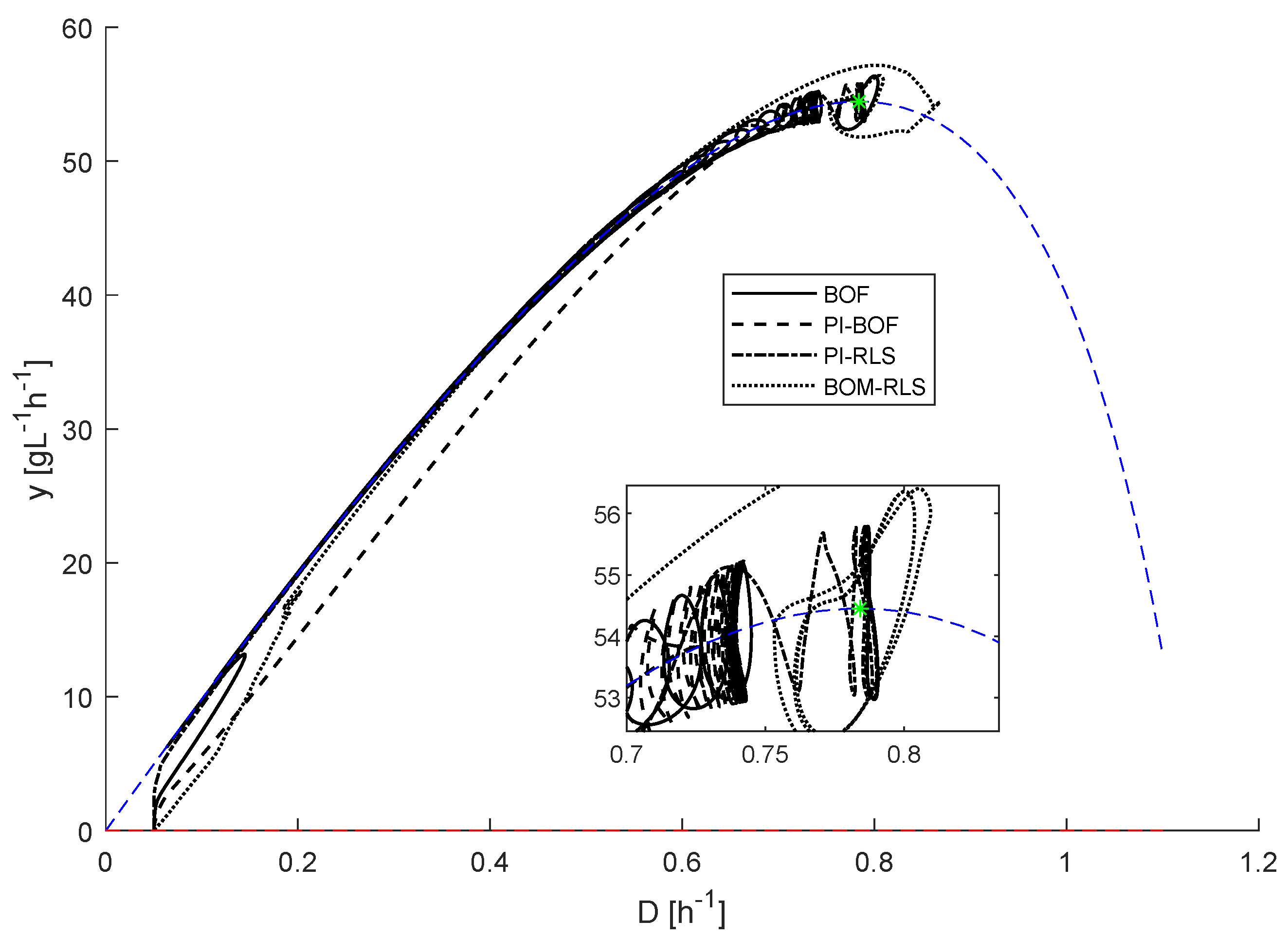
4.4. Numerical Results

The several ES algorithms designed in Section 4.1, Section 4.2 and Section 4.3 are now compared when optimizing the biomass production, $y=Dx$ in the presence of different kinetic structures, such as Monod, Haldane, and Contois. First, Figure 8 and Figure 9 show the results of the application of the BOF, PI-BOF, PI-RLS, and BOM extremum seeking methods to the Monod case.

Not surprisingly, BOM and PI-BOF algorithms achieved the fastest convergences of, respectively, 50 and 25 h; PI-RLS and BOF converged within, respectively, 300 and more than 1000 h. However, Figure 8 and Figure 9 also show that PI-BOF reaches the optimum neighborhood with a significant offset (see the zoom box of Figure 9) while the convergence of BOM, even if slightly slower, is more accurate.

These first results are confirmed in the Haldane case in Figure 10 and Figure 11, even if the BOM algorithm performs better this time in terms of convergence time and accuracy, and PI-RLS and BOF respectively converged within 200 and 600 h.

Nevertheless, the algorithm behaviors are interestingly emphasized when using the Contois kinetic law, as shown in Figure 12. While the performances of the BOM and BOF strategies are identical to the previous cases, PI-BOF and PI-RLS show larger offsets with respect to optimal state and dilution rate equilibria. This can be attributed to the gradient values which are, however, still very close to 0. In the particular case of Contois kinetics, the convergence diagram of Figure 13 shows that the equilibrium slopes are much smoother compared to the previous Monod and Haldane cases. A small shift in a close neighborhood of the optimum, keeping $y\approx y^{*}$, may then lead to important offsets on the dilution rate and therefore on the states.

Observations based on these several numerical illustrations can be summarized as follows:

• The BOM strategy is by far the most accurate since it allows taking unknown output dynamics into account.
• The PI-BOF strategy allows solving the extremum seeking problem almost instantaneously and therefore provides the fastest convergence, but as a drawback, has a technically inherent and significant offset (see [78]).
• The PI-RLS strategy presents a smaller offset and is overall easy to implement while achieving reasonable convergence times.
• The BOF strategy, even if in the original it was the most intuitive and easiest to implement method, presents several drawbacks, such as long convergence time, tedious parameter tuning, and possible offsets.

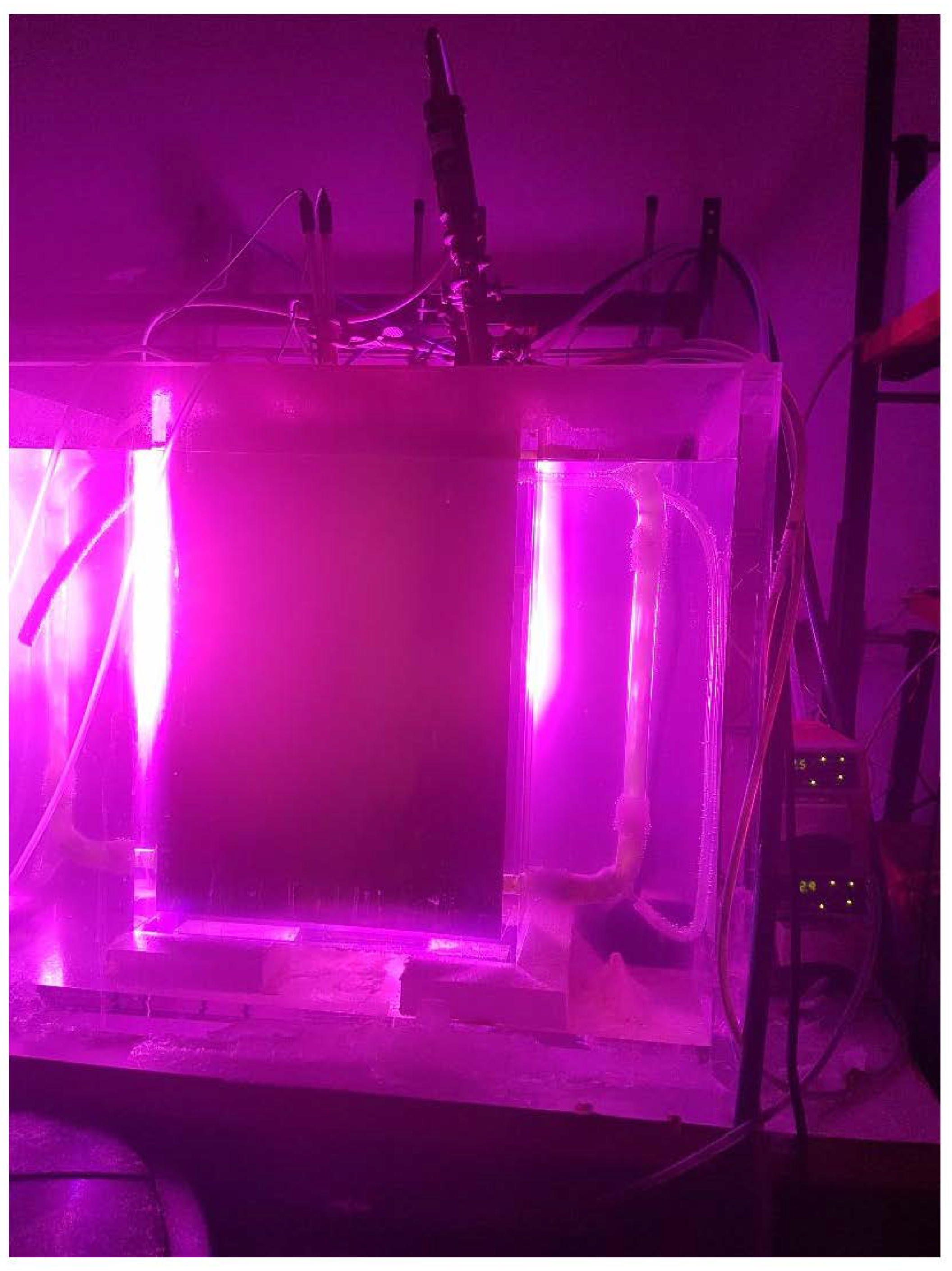
5. Real-Life Applications: Microalgae Production Optimization

Most of the publications discussed in this review propose simulation results in order to provide some practical assessment and recommendations in view of future experimental implementation. Among the very few experimental validations reported in the literature, two investigations aiming at maximizing microalgae culture productivity by extremum seeking have been proposed in [75,102].

5.1. Microalgae Growth Rate Optimization

In [75], the method consists of modulating the pH to optimize the measured Nannochloropsis Oculata microalgae biomass growth rate, using the $C{O}_2$ “flow as actuator” in an internal loop regulating the pH. In this regard, a perturbation-based filter bank ES was first designed in a simulation and some tuning guidelines were suggested as follows:

• Quantification of the system dynamics and uncertainties;
• Selection of the dither frequency, and to some extent, its structure;
• Trial and error optimization routine defining the high-pass filter cut-off frequency;
• If the level of noise requires it, determination of the low-pass filter cut-off frequency.

The use of a low-pass filter should, however, be avoided as much as possible since it is a source of convergence slow-down (the reader may refer to the time-scale separations explained in Section 2.2.1). Following the initial simulation results, an experimental validation with a 27-liter tubular bubble column photobioreactor reproducing a down-scaled industrial process was achieved. The main results show that the ES scheme managed to bring the system to an acceptable pH range, as predicted by other works from the literature.

5.2. Microalgae Productivity Optimization

In a recent experimental investigation achieved by the authors [102], a RLS-ES controller was designed, assuming a Hammerstein representation between the biomass X of the strain Dunaliella tertiolecta, as measured output, and the dilution rate D, assumed to be the sole input. The biomass productivity, defined as $P=DX$ is then maximized and its gradient estimate is provided by:

$$\begin{array}{}\mathrm{(34a)}& \hfill \widehat{\frac{\partial P}{\partial D}}& =\widehat{\frac{\partial DX}{\partial D}}\hfill \mathrm{(34b)}& \hfill & =\widehat{X}+\widehat{\frac{\partial X}{\partial D}}\hfill \mathrm{(34c)}& \hfill & =\widehat{X}+D\widehat{m}\hfill \mathrm{(34d)}& \hfill & =2\widehat{m}D+\widehat{b}\hfill \end{array}$$

assuming the static mapping $X\left(k\right)=mD\left(k\right)+b$. It must be noticed that a filtered biomass variable $X_f$ may also be considered leading to similar performance. The estimated optimal productivity and dilution rate can be inferred as:

$$\begin{array}{}\mathrm{(35a)}& \hfill {\widehat{D}}^{*}& =-\frac{\widehat{b}}{2\widehat{m}}\hfill \mathrm{(35b)}& \hfill {\widehat{P}}^{*}& =-\frac{\widehat{b^2}}{4\widehat{m}}\hfill \end{array}$$

The experimental set-up was a 13-liter flat photobioreactor shown in Figure 14. For more details regarding the monitoring devices, the reader may refer to [102].

A ten-day experiment was performed, leading to the results presented in Figure 15, Figure 16 and Figure 17, wherein the gradient was indeed pushed to zero on average within 4 days leading to the maximum productivity level. Figure 17 compares the predicted static map with the convergence results, proving the method’s accuracy.

Following these encouraging first results, further experiments were scheduled, using the BOM-ES method from Section 4.3, and are currently in validation.

6. Conclusions

During the last two decades, extremum seeking (ES) has become a very popular research subject, and has lead to an increasing number of real-life applications to electro-mechanical systems. The application of ES to biosystems is, however, quite tedious due to the uncertain nature of the “living” in a broad sense, and the slow dynamics of the bioprocesses. In view of the model uncertainties, model-free ES appears as an appealing approach to achieve “plug-and-play” process optimization. Even if the seminal perturbation-based techniques based on the use of high and low pass filtering provide guaranteed results if a correct parameterization is selected, the three time-scale separations entail very lengthy convergence times. Most of the recent ES approaches therefore focus on ES convergence issues, acting on the controller structure and design, on parameter estimation, or on the dither signal definition. This review paper discussed some of these techniques using an illustrative simulation example, where the biomass production of a simple microbial growth model was maximized considering several kinetic structures with different complexity levels and corresponding static maps.

Only a few real-life applications of ES to bioprocesses are described in the open literature, namely, those to continuous microalgae cultures in photo-bioreactors. Hopefully, these experimental studies will pave the way for future studies at pilot and industrial scales.

References

1. Darby, M.L.; Nikolaoub, M.; Jones, J.; Nicholson, D. RTO: An overview and assessment of current practice. J. Process Control 2011, 21, 874–884. [Google Scholar] [CrossRef]
2. Chachuat, B.; Srinivasan, B.; Bonvin, D. Adaptation Strategies for Real-time Optimization. Comput. Chem. Eng. 2009, 33, 1557–1567. [Google Scholar] [CrossRef]
3. Srinivasan, B.; Bonvin, D. Interplay between Identification and Optimization in Run-to-run Optimization Schemes. In Proceedings of the 2002 American Control Conference (IEEE Cat. No. CH37301), Anchorage, AK, USA, 8–10 May 2002; pp. 2174–2179. [Google Scholar]
4. Marchetti, A.; Chachuat, B.; Bonvin, D. Modifier-Adaptation Methodology for Real-Time Optimization. Ind. Eng. Chem. Res. 2009, 48, 6022–6033. [Google Scholar] [CrossRef] [Green Version]
5. Gao, W.; Wenzel, S.; Engell, S. A reliable modifier-adaptation strategy for real-time optimization. Comput. Chem. Eng. 2016, 91, 318–328. [Google Scholar] [CrossRef] [Green Version]
6. Skogestad, S. Self-optimizing Control: The Missing Link between Steady-state Optimization and Control. Comput. Chem. Eng. 2000, 24, 569–575. [Google Scholar] [CrossRef] [Green Version]
7. Ariyur, K.B.; Krstic, M. Real-Time Optimization by Extremum-Seeking Control; Wiley-Interscience, Ed.; John Wiley & Sons, Inc.: Hoboken, NJ, USA, 2003. [Google Scholar]
8. Tan, Y.; Moase, W.; Manzie, C.; Nesic, D.; Mareels, I. Extremum Seeking from 1922 to 2010. In Proceedings of the 29th Chinese Control Conference, Beijing, China, 29–31 July 2010; pp. 14–26. [Google Scholar]
9. Krstic, M. Extremum Seeking Control. In Encyclopedia of Systems and Control; Baillieul, J., Samad, T., Eds.; Springer: London, UK, 2020. [Google Scholar]
10. Srinivasan, B.; Primus, C.J.; Bonvin, D.; Ricker, N.L. Run-to-run optimization via control of generalized constraints. Control Eng. Pract. 2001, 9, 911–919. [Google Scholar] [CrossRef] [Green Version]
11. Francois, G.; Srinivasan, B.; Bonvin, D. Use of measurements for enforcing the necessary conditions of optimality in the presence of constraints and uncertainty. J. Process Control 2005, 15, 701–712. [Google Scholar] [CrossRef] [Green Version]
12. Engell, S. Feedback control for optimal process operation. J. Process Control 2007, 17, 203–219. [Google Scholar] [CrossRef]
13. Adetola, V.; Guay, M. Integration of real-time optimization and model predictive control. J. Process Control 2010, 20, 125–133. [Google Scholar] [CrossRef]
14. De Souza, G.; Odloak, D.; Zanin, A.C. Real time optimization (RTO) with model predictive control (MPC). Comput. Chem. Eng. 2010, 34, 1996–2006. [Google Scholar] [CrossRef]
15. Scheinker, A.; Krstić, M. Model-Free Stabilization by Extremum Seeking; Springer: Berlin/Heidelberg, Germany, 2017. [Google Scholar]
16. Leblanc, M. Sur l’électrification des chemins de fer au moyen de courants alternatifs de fréquence élevée. Revue Générale De L’Électricité 1922, 12, 275–277. [Google Scholar]
17. Kazakevich, V.V. Technique of Automatic Control of Different Processes to Maximum or to Minimum. Avtorskoe Svidetelstvo USSR Patent 66335, 25 November 1943. [Google Scholar]
18. Draper, C.S.; Li, Y.T. Principales of Optimalizing Control Systems and an Application to the Internal Combustion Engine. In Optimal and Selfoptimizing Control; Oldenburger, R., Ed.; The MIT Press: Boston, MA, USA, 1951. [Google Scholar]
19. Morosanov, I.S. Method of extremum control. Autom. Remote Control 1957, 18, 1077–1092. [Google Scholar]
20. Meerkov, S.M. Asymptotic methods for investigating a class of forced states in extremal systems. Autom. Remote Control 1967, 12, 1916–1920. [Google Scholar]
21. Blackman, P.F. Extremum-Seeking Regulators. In An Exposition of Adaptive Control; Westcott, J.H., Ed.; The Macmillan Company: New York, NY, USA, 1962. [Google Scholar]
22. Luxat, J.; Lees, L. Stability of peak-holding control systems. IEEE Trans. Ind. Electron. Control Instrum. 1971, 11–15. [Google Scholar] [CrossRef]
23. Korovin, S.; Utkin, V. Using sliding modes in static optimization and nonlinear programming. Automatica 1974, 10, 525–532. [Google Scholar] [CrossRef]
24. Wang, H.H.; Krstic, M. Extremum seeking for limit cycle minimization. IEEE Trans. Autom. Control 2000, 45, 2432–2437. [Google Scholar] [CrossRef] [Green Version]
25. Aström, K.J.; Wittenmark, B. Adaptive Control, 2nd ed.; Addison-Wesley Publishing Company, Inc.: Boston, MA, USA, 1995. [Google Scholar]
26. Leyva, R.; Alonso, C.; Queinnec, I.; Cid-Pastor, A.; Lagrange, D.; Martinez-Salamero, L. MPPT of photovoltaic systems using extremum-seeking control. IEEE Trans. Aerosp. Electron. Syst. 2006, 42, 249–258. [Google Scholar] [CrossRef]
27. Ghaffari, A.; Krstić, M.; Seshagiri, S. Power optimization for photovoltaic microconverters using multivariable newton-based extremum seeking. IEEE Trans. Control Syst. Technol. 2014, 22, 2141–2149. [Google Scholar] [CrossRef]
28. Chichka, D.F.; Speyer, J.L.; Fanti, C.; Park, C.G. Peak-seeking control for drag reduction in formation flight. J. Guid. Control. Dyn. 2006, 29, 1221–1230. [Google Scholar] [CrossRef] [Green Version]
29. Van der Meulen, S.; De Jager, B.; Veldpaus, F.; Van der Noll, E.; Van der Sluis, F.; Steinbuch, M. Improving continuously variable transmission efficiency with extremum seeking control. IEEE Trans. Control Syst. Technol. 2011, 20, 1376–1383. [Google Scholar] [CrossRef]
30. Hellström, E.; Lee, D.; Jiang, L.; Stefanopoulou, A.G.; Yilmaz, H. On-board calibration of spark timing by extremum seeking for flex-fuel engines. IEEE Trans. Control Syst. Technol. 2013, 21, 2273–2279. [Google Scholar] [CrossRef]
31. Koeln, J.P.; Alleyne, A.G. Optimal subcooling in vapor compression systems via extremum seeking control: Theory and experiments. Int. J. Refrig. 2014, 43, 14–25. [Google Scholar] [CrossRef]
32. Burns, D.J.; Weiss, W.K.; Guay, M. Realtime setpoint optimization with time-varying extremum seeking for vapor compression systems. In Proceedings of the 2015 American Control Conference (ACC), Chicago, IL, USA, 1–3 July 2015; pp. 974–979. [Google Scholar]
33. Ghaffari, A.; Krstić, M.; Seshagiri, S. Power optimization and control in wind energy conversion systems using extremum seeking. IEEE Trans. Control Syst. Technol. 2014, 22, 1684–1695. [Google Scholar] [CrossRef]
34. Shahriari, Z. An Extremum Seeking Control System for Control of RF Cavity Resonators. Ph.D. Thesis, School of Mechatronic Systems Engineering, Simon Fraser University, Surrey, BC, Canada, 2016. [Google Scholar]
35. Leewe, R.; Shahriari, Z.; Fong, K.; Moallem, M. Resonance frequency tuning of an RF cavity through sliding mode extremum seeking. Nucl. Instruments Methods Phys. Res. Sect. A Accel. Spectrometers Detect. Assoc. Equip. 2018, 902, 70–75. [Google Scholar] [CrossRef]
36. Dinçmen, E.; Altınel, T. An emergency braking controller based on extremum seeking with experimental implementation. Int. J. Dyn. Control 2018, 6, 270–283. [Google Scholar] [CrossRef]
37. Wang, H.H.; Krstic, M.; Bastin, G. Optimizing Bioreactors by Extremum-seeking. Int. J. Adapt. Control Signal Process. 1999, 13, 651–669. [Google Scholar] [CrossRef]
38. Marcos, N.I.; Guay, M.; Dochain, D. Output Feedback Adaptive Extremum Seeking Control for a Continuous Stirred Tank Bioreactor with Monod’s Kinetics. J. Process Control 2004, 14, 807–818. [Google Scholar] [CrossRef]
39. Akesson, M.; Hagander, P.; Axelsson, J.P. A probing feeding strategy for Escherichia coli cultures. Biotechnol. Tech. 1999, 13, 523–528. [Google Scholar] [CrossRef]
40. Akesson, M.; Hagander, P.; Axelsson, J.P. Avoiding acetate accumulation in Escherichia Coli Cult. Using Feedback Control Glucose Feed. Biotechnol. Bioeng. 2001, 73, 223–230. [Google Scholar] [CrossRef]
41. Teel, A.R.; Popović, D. Solving smooth and nonsmooth multivariable extremum seeking problems by the methods of nonlinear programming. In Proceedings of the 2001 American Control Conference. (Cat. No. 01CH37148), Arlington, VA, USA, 25–27 June 2001; pp. 2394–2399. [Google Scholar]
42. Guay, M.; Zhang, T. Adaptive extremum seeking control of nonlinear dynamic systems with parametric uncertainties. Automatica 2003, 39, 1283–1293. [Google Scholar] [CrossRef]
43. Zhang, T.; Guay, M.; Dochain, D. Adaptive Extremum Seeking Control of Continuous Stirred-Tank Bioreactors. AIChE J. 2004, 49, 113–123. [Google Scholar] [CrossRef]
44. Krstic, M.; Kanellakopoulos, I.; Kokotovic, P. Nonlinear and Adaptive Control Design; Wiley and Sons: New York, NY, USA, 1995. [Google Scholar]
45. Ioannou, P.; Sun, J. Robust Adaptive Control; Prentice-Hall: Eaglewood Cliffs, NJ, USA, 1996. [Google Scholar]
46. Khalil, H. Nonlinear Systems; Prentice-Hall: Upper Saddle River, NJ, USA, 2002. [Google Scholar]
47. Dochain, D.; Perrier, M.; Guay, M. Extremum seeking control and its application to process and reaction systems: A survey. Math. Comput. Simul. 2011, 82, 369–380. [Google Scholar] [CrossRef]
48. Titica, M.; Dochain, D.; Guay, M. Adaptive Extremum-seeking Control of Fed-batch Bioreactors. Eur. J. Control 2003, 9, 618–631. [Google Scholar] [CrossRef]
49. Titica, M.; Dochain, D.; Guay, M. Real-time Optimization of Fed-batch Bioreactors via Adaptive Extremum-seeking Control. Chem. Eng. Res. Des. 2003, 81, 1289–1295. [Google Scholar] [CrossRef]
50. Marcos, N.; Guay, M.; Dochain, D.; Zhang, T. Adaptive extremum-seeking control of a continuous stirred tank bioreactor with Haldane’s Kinetics. J. Process Control 2004, 14, 317–328. [Google Scholar] [CrossRef]
51. Cougnon, P.; Dochain, D.; Guay, M.; Perrier, M. On-line optimization of fedbatch bioreactors by adaptive extremum seeking control. J. Process Control 2011, 21, 1526–1532. [Google Scholar] [CrossRef]
52. Dewasme, L.; Vande Wouwer, A. Adaptive Extremum-seeking Control Applied to Productivity Optimization in Yeast Fed-batch cultures. IFAC World Congr. 2008, 41, 9713–9718. [Google Scholar] [CrossRef] [Green Version]
53. Sonnleitner, B.; Käppeli, O. Growth of Saccharomyces Cerevisiae Is Control. Its Ltd. Respir. Capacit: Formulation Verif. A Hypothesis. Biotechnol. Bioeng. 1986, 28, 927–937. [Google Scholar] [CrossRef]
54. Guay, M.; Dochain, D.; Perrier, M. Adaptive extremum seekingcontrol of continuous stirred tank bioreactors with unknown growth kinetics. Automatica 2004, 40, 881–888. [Google Scholar] [CrossRef]
55. Lara-Cisneros, G.; Femat, R.; Dochain, D. An extremum seeking approach via variable-structure control for fed-batch bioreactors with uncertain growth rate. J. Process Control 2014, 24, 663–671. [Google Scholar] [CrossRef]
56. Lara-Cisneros, G.; Aguilar-López, R.; Femat, R. On the dynamic optimization of methane production in anaerobicdigestion via extremum-seeking control approach. Comput. Chem. Eng. 2015, 75, 49–59. [Google Scholar] [CrossRef]
57. Vargas, A.; Moreno, J.; Vande Wouwer, A. Super-twisting estimation of a virtual output for extremum-seeking output feedback control of bioreactors. J. Process Control 2015, 35, 41–49. [Google Scholar] [CrossRef]
58. Lara-Cisneros, G.; Femat, R.; Dochain, D. Robust sliding mode-based extremum-seeking controller for reaction systems via uncertainty estimation approach. Int. J. Robust Nonlinear Control 2017, 27, 3218–3235. [Google Scholar] [CrossRef]
59. Lara-Cisneros, G.; Dochain, D.; Alvarez-Ramírez, J. Model based extremum-seeking controller via modelling- errorcompensation approach. J. Process Control 2019, 80, 193–201. [Google Scholar] [CrossRef]
60. Guay, M.; Peters, N. Real-time dynamic optimization of nonlinear systems: A flatness-based approach. Comput. Chem. Eng. 2006, 30, 709–721. [Google Scholar] [CrossRef]
61. Peters, N.; Guay, M.; DeHaan, D. Real-time dynamic optimization of batch systems. J. Process Control 2007, 17, 261–271. [Google Scholar] [CrossRef]
62. Guay, M.; Adetola, V. Adaptive economic optimising model predictive control of uncertain nonlinear systems. Int. J. Control 2013, 86, 1425–1437. [Google Scholar] [CrossRef]
63. Landau, I.D.; Dugard, L. Commande Adaptative. Aspects Pratiques et Théoriques; Masson: Paris, France, 1986. [Google Scholar]
64. Krstic, M.; Wang, H.H. Stability of Extremum Seeking Feedback for General Nonlinear Dynamic Systems. Automatica 2000, 36, 595–601. [Google Scholar] [CrossRef]
65. Nguang, S.K.; Chen, X.D. Extremum seeking schemes for continuous fermentation processes described by an unstructured fermentation model. Bioprocess Eng. 2000, 23, 417–420. [Google Scholar] [CrossRef]
66. Simeonov, I.; Noykova, N.; Stoyanov, S. Modelling and extremum seeking control of the anaerobic digestion. IFAC Proc. Vol. 2004, 37, 289–294. [Google Scholar] [CrossRef]
67. Chioua, M.; Srinivasan, B.; Guay, M.; Perrier, M. Dependence of the error in the optimal solution of perturbation-based extremum seeking methods on the excitation frequency. Can. J. Chem. Eng. 2007, 85, 447–453. [Google Scholar] [CrossRef]
68. Tan, Y.; Nesic, D.; Mareels, I. On the Choice of Dither in Extremum Seeking Systems: A Case Study. Automatica 2008, 44, 1446–1450. [Google Scholar] [CrossRef]
69. Krstic, M. Performance Improvement and Limitations in Extremum Seeking Control. Syst. Contr. Lett. 2000, 39, 313–326. [Google Scholar] [CrossRef]
70. Chioua, M.; Srinivasan, B.; Perrier, M.; Guay, M. Improving convergence of perturbation-based extremum seeking methods for a class of differentially flat systems. IFAC Proc. Vol. 2007, 40, 270–275. [Google Scholar] [CrossRef]
71. Simeonov, I.; Stoyanov, S. Modelling and Extremum Seeking Control of a Cascade of Two Anaerobic Bioreactors. Int. J. Bioautom. 2011, 15, 13–24. [Google Scholar]
72. Barbu, M.; Ceanga, E.; Vilanova, R.; Caraman, S.; Ifrim, G. Extremum-seeking contro approach based on the influent variability for anaerobic digestion optimization. IFAC Pap. 2017, 50, 12623–12628. [Google Scholar] [CrossRef]
73. Pessoa, R.; Mendes, F.; Oliveira, T.R.; Oliveria-Esquerre, K.; Krstic, M. Numerical optimization based on generalized extremum seeking for fast methane production by a modified ADM1. J. Process Control 2019, 84, 56–69. [Google Scholar] [CrossRef]
74. Dewasme, L.; Srinivasan, B.; Perrier, M.; Vande Wouwer, A. Extremum-seeking algorithm design for fed-batch cultures of microorganisms with overflow metabolism. J. Process Control 2011, 21, 1092–1104. [Google Scholar] [CrossRef]
75. Deschênes, J.S.; St-Onge, P.N.; Collin, J.C.; Tremblay, R. Extremum Seeking Control of Batch Cultures of Microalgae Nannochloropsis Oculata in Pre-Industrial Scale Photobioreactors. IFAC Proc. Vol. 2012, 45, 585–590. [Google Scholar] [CrossRef]
76. Sastry, S.; Bodson, M. Adaptive Control: Stability, Convergence and Robustness; Prentice Hall Information and System Sciences Series; Prentice Hall: Englewood Cliffs, NJ, USA, 1989. [Google Scholar]
77. Chioua, M.; Srinivasan, B.; Guay, M.; Perrier, M. Performance Improvement of Extremum Seeking Control using Recursive Least Square Estimation with Forgetting Factor. IFAC Pap. 2016, 49, 424–429. [Google Scholar] [CrossRef]
78. Guay, M.; Dochain, D. A time-varying extremum-seeking control approach. Automatica 2015, 51, 356–363. [Google Scholar] [CrossRef]
79. de Maré, L.; Andersson, M.; Hagander, P. Probing control of glucose feeding in Vibrio cholerae cultivations. Bioprocess Biosyst. Eng. 2003, 25, 221–228. [Google Scholar] [CrossRef] [PubMed]
80. Johnsson, O.; Andersson, J.; Johnsson, C. Probing control in B. licheniformis fermentations. IFAC Proc. Vol. 2011, 44, 7132–7137. [Google Scholar] [CrossRef] [Green Version]
81. Henes, B.; Sonnleitner, B. Controlled fed-batch by tracking the maximal culture capacity. J. Biotechnol. 2007, 132, 118–126. [Google Scholar] [CrossRef]
82. Velut, S.; Castan, A.; Short, K.; Axelsson, J.; Hagander, P.; Zditosky, B.; Rysenga, C.; de Maré, L.; Haglund, J. Influence of bioreactor scale and complex medium on probing control of glucose feeding in cultivations of recombinant strains of Escherichia coli. Biotechnol. Bioeng. 2007, 97, 816–824. [Google Scholar] [CrossRef] [PubMed]
83. Feudjio Letchindjio, C.G.; Dewasme, L.; Deschênes, J.S.; Vande Wouwer, A. An Extremum Seeking Strategy Based on Block-Oriented Models: Application to Biomass Productivity Maximization in Microalgae Cultures. Ind. Eng. Chem. Res. 2019, 58, 13481–13494. [Google Scholar] [CrossRef]
84. Guay, M.; Dochain, D. A proportional integral extremum-seeking control approach. IFAC Proc. Vol. 2014, 47, 377–382. [Google Scholar] [CrossRef] [Green Version]
85. Guay, M.; Dochain, D. A proportional-integral extremum-seeking controller design technique. Automatica 2017, 77, 61–67. [Google Scholar] [CrossRef]
86. Guay, M. A Perturbation-Based Proportional Integral Extremum-Seeking Control Approach. IEEE Trans. Autom. Control 2016, 61, 3370–3381. [Google Scholar] [CrossRef]
87. Burns, D.J.; Laughman, C.R.; Guay, M. Proportional-Integral Extremum Seeking for Vapor Compression Systems. IEEE Trans. Control Syst. Technol. 2020, 28, 403–412. [Google Scholar] [CrossRef]
88. Tan, Y.; Nesic, D.; Mareels, I. On Non-local Stability Properties of Extremum Seeking Control. Automatica 2006, 42, 889–903. [Google Scholar] [CrossRef] [Green Version]
89. Moase, W.; Manzie, C. Fast extremum-seeking for Wiener-Hammerstein plants. Automatica 2012, 48, 2433–2443. [Google Scholar] [CrossRef]
90. Moase, W.; Manzie, C. Semi-Global Stability Analysis of Observer-Based Extremum-Seeking for Hammerstein Plants. IEEE Trans. Autom. Control 2012, 57, 1685–1695. [Google Scholar] [CrossRef]
91. Sharafi, J.; Moase, W.H.; Manzie, C. Fast extremum seeking on Hammerstein plants: A model-based approach. Automatica 2015, 59, 171–181. [Google Scholar] [CrossRef]
92. Atta, K.T.; Guay, M. Adaptive amplitude fast proportional integral phasor extremum seeking control for a class of nonlinear systems. J. Process Control 2019, 83, 147–154. [Google Scholar] [CrossRef]
93. Tan, Y.; Nesic, D.; Mareels, I.; Astolfi, A. On Global Extremum Seeking in the Presence of Local Extrema. Automatica 2009, 45, 245–251, Brief Paper. [Google Scholar] [CrossRef]
94. Giri, F.; Bai, E.W. Block-Oriented Nonlinear System Identification; Springer: Berlin/Heidelberg, Germany, 2010; Volume 1. [Google Scholar]
95. Ljung, L.; Söderström, T. Theory and Practice of Recursive Identification; MIT Press: Cambridge, MA, USA, 1983. [Google Scholar]
96. Kortmann, M.; Unbehauen, H. Identification methods for nonlinear MISO systems. IFAC Proc. Vol. 1987, 20, 233–238. [Google Scholar] [CrossRef]
97. Landau, I.D.; Lozano, R.; M’Saad, M.; Karimi, A. Adaptive Control: Algorithms, Analysis and Applications; Springer Science & Business Media: Berlin/Heidelberg, Germany, 2011. [Google Scholar]
98. Bastin, G.; Nesic, D.; Tan, Y.; Mareels, I. On extremum seeking in bioprocesses with multivalued cost functions. Biotechnol. Prog. 2009, 25, 683–689. [Google Scholar] [CrossRef]
99. Trollberg, O.; Jacobsen, E. Greedy Extremum Seeking Control with Applications to Biochemical Processes. IFAC-PaperOnLine 2016, 49, 109–114. [Google Scholar] [CrossRef]
100. Atta, K.; Johansson, A.; Gustafsson, T. Extremum seeking control based on phasor estimation. Syst. Control Lett. 2015, 85, 37–45. [Google Scholar] [CrossRef]
101. Cormen, T. Introduction to Algorithms; MIT Press: Cambridge, MA, USA, 2009. [Google Scholar]
102. Feudjio Letchindjio, C.G.; Dewasme, L.; Vande Wouwer, A. Extremum-Seeking for micro-algae biomass productivity maximization: An experimental validation. IFAC-PapersOnLine 2019, 52, 281–286. [Google Scholar] [CrossRef]
Figure 1. Extremum seeking control (ESC) basic scheme.
Processes 08 01209 g001
Figure 2. Extremum seeking with bank of filters.
Processes 08 01209 g002
Figure 3. Extremum seeking with a recursive estimator.
Processes 08 01209 g003
Figure 4. Extremum seeking as a simple output feedback.
Processes 08 01209 g004
Figure 5. Proportional-integral extremum seeking control scheme (PIESC).
Processes 08 01209 g005
Figure 6. Block-oriented recursive extremum seeking control strategy - reproduced with permission (with slight modifications) from [83].
Processes 08 01209 g006
Figure 7. Extremum seeking feedback scheme.
Processes 08 01209 g007
Figure 8. Application of the BOF, PI-BOF, PI-RLS, and BOM extremum seeking methods to optimize biomass productivity of microbial growth represented by model (3) with Monod kinetics—state, input, and output time evolutions.
Processes 08 01209 g008
Figure 9. Application of the BOF, PI-BOF, PI-RLS, and BOM extremum seeking methods to optimize biomass productivity of microbial growth represented by model (3) with Monod kinetics—convergence diagram.
Processes 08 01209 g009
Figure 10. Application of the BOF, PI-BOF, PI-RLS, and BOM extremum seeking methods to optimize biomass productivity of microbial growth represented by model (3) with Haldane kinetics—state, input, and output time evolutions.
Processes 08 01209 g010
Figure 11. Application of the BOF, PI-BOF, PI-RLS, and BOM extremum seeking methods to optimize biomass productivity of microbial growth represented by model (3) with Haldane kinetics—convergence diagram.
Processes 08 01209 g011
Figure 12. Application of the BOF, PI-BOF, PI-RLS, and BOM extremum seeking methods to optimize biomass productivity of microbial growth represented by model (3) with Contois kinetics—state, input, and output time evolutions.
Processes 08 01209 g012
Figure 13. Application of the BOF, PI-BOF, PI-RLS, and BOM extremum seeking methods to optimize biomass productivity of microbial growth represented by model (3) with Contois kinetics—convergence diagram.
Processes 08 01209 g013
Figure 14. Lab-scale flat photobioreactor—reproduced with permission from [102].
Processes 08 01209 g014
Figure 15. Experimental validation of RLS-ES on Dunaliella tertiolecta continuous cultures: productivity and dilution rate evolutions—reproduced with permission from [102].
Processes 08 01209 g015
Figure 16. Experimental validation of RLS-ES on Dunaliella tertiolecta continuous cultures: gradient evolution—reproduced with permission (and slight modifications) from [102].
Processes 08 01209 g016
Figure 17. Experimental validation of RLS-ES on Dunaliella tertiolecta continuous cultures: productivity and dilution phase plan—reproduced with permission from [102].
Processes 08 01209 g017