Article

Application of Transformation Matrices to the Solution of Population Balance Equations

1
Institute of Solids Process Engineering and Particle Technology, Hamburg University of Technology, Denickestrasse 15, 21073 Hamburg, Germany
2
Department of Mathematics, Indian Institute of Technology Kharagpur, Kharagpur 721302, India
*
Author to whom correspondence should be addressed.
Processes 2019, 7(8), 535; https://doi.org/10.3390/pr7080535
Submission received: 25 July 2019 / Revised: 8 August 2019 / Accepted: 11 August 2019 / Published: 14 August 2019
(This article belongs to the Special Issue Chemical Process Design, Simulation and Optimization)

Abstract

:
The development of algorithms and methods for modelling flowsheets in the field of granular materials has a number of challenges. The difficulties are mainly related to the inhomogeneity of solid materials, requiring a description of granular materials using distributed parameters. To overcome some of these problems, an approach with transformation matrices can be used. This allows one to quantitatively describe the material transitions between different classes in a multidimensional distributed set of parameters, making it possible to properly handle dependent distributions. This contribution proposes a new method for formulating transformation matrices using population balance equations (PBE) for agglomeration and milling processes. The finite volume method for spatial discretization and the second-order Runge–Kutta method were used to obtain the complete discretized form of the PBE and to calculate the transformation matrices. The proposed method was implemented in the flowsheet modelling framework Dyssol to demonstrate and prove its applicability. Hence, it was revealed that this new approach allows the modelling of complex processes involving materials described by several interconnected distributed parameters, correctly taking into consideration their interdependency.

Graphical Abstract

1. Introduction

Bulk materials typically consist of individual non-uniform particles having different parameters, which vary in a certain range. These parameters are referred to as distributed and include, for example, the diameters of particles, their densities, or porosities. Although these parameters can physically be fairly accurately described by continuous distribution functions, such a representation is not always convenient for numerical analysis and modelling. Therefore, in practice, the continuously distributed material parameter space is discretized into shorter intervals, usually called classes. Each class is assigned a quantity of material, whose parameters fall into this particular interval. In this case, the distribution of the parameter of the entire material in this class is narrowed down from a continuous distribution function to a single value, for example, the average value of this class. Thus, it is assumed that all the particles inside have the same value of the parameter. Therefore, a simulation system can operate using a finite number of parameter values, which (if the number of classes is sufficient) accurately describe the original distribution.
Despite the fact that most models in solids processing technology consider particle size distribution as one of the main material parameters, many of them additionally incorporate various other attributes. For example, the shape and orientation of primary particles are important in crystallization processes [1]; the size and yield strength of the colliding granules can be considered as parameters for wet granulation models [2]; the distributions of granules by porosity and saturation are important for breakage rate in some apparatuses [3]; and the moisture content of particles plays a significant role in dryers [4].
Such a diversity of models and their parameters makes the simulation process much more challenging when trying to combine their different types in a single flowsheet. The main problem here is that each unit is usually being developed to consider only a limited number of distributed parameters which are important for its model, neglecting others. Moreover, the usual approach to develop models involves a direct calculation of the distributed parameters at the outlet of a unit. As a result, if the material is additionally described by some secondary distributed parameters, information about them and their dependencies may be lost during the simulation.
For example, consider a flowsheet where a screen and a dryer are connected in series, and the solid phase is distributed according to particle size and moisture content. In this case, the screen unit, usually performing separation of particles only according to size, will fail to determine their moisture properly, which is important for the dryer.
To handle this issue, Pogodda [5] introduced an approach using transformation matrices and implemented it into the SolidSim simulation environment. Later, Dosta [6] and Skorych et al. [7] extended this technique for the dynamic flowsheet simulation using the Euler method. Transformation matrices in this approach describe the laws of mass transfer between all classes of the distribution. Their application, instead of explicit calculation of output flows, enables the usage of more material parameters in a proper way and implicitly preserves information about all secondary distributions and their dependencies at any time point in the unit.

1.1. Flowsheet Simulation of Solid Phase Processes

Nowadays, flowsheet simulation software is commonly used to aid with design, planning, optimization, and testing in chemical engineering [8]. Usually it can help with the minimization of operation costs, troubleshooting, increasing throughput and product quality, and generally provides a better understanding of the process. However, despite the fact that flowsheet simulation of fluid processes has already been state of the art for many decades [9], generally applicable systems for modelling granular materials began to appear only recently and are now being actively developed. This arises from the complexity of description and handling of the solid phase. In contrast to fluids, it requires treatment of distributed parameters, such as particle size, internal porosity or moisture content. Moreover, these distributions can be interrelated, which requires even more advanced methods to treat them properly and preserve their interconnection during the simulation.
Currently, flowsheet modelling systems that can work with the solid phase are being actively developed. Among them may for example be mentioned:
  • Aspen Plus [10], which is actively used in chemical industry as well as for simulation of polymers, minerals, metals etc.
  • gPROMS FormulatedProducts [11], as a part of gPROMS platform, especially designed to investigate solid phase processes.
  • JKSimMet [12], which is a flowsheeting software for simulation of comminution and classification circuits in the mineral processing industry.
  • The HSC Sim [13] module of HSC Chemistry software intended for modelling various processes in chemistry, metallurgy, and mineralogy.
  • CHEMCAD [14], which was developed to simulate chemical processes with limited consideration of the solid phase.
  • Dyssol [7], a flowsheet simulation system designed to simulate complex dynamic processes in solids processing technology, developed within a research collaboration founded by the German Research Foundation.
Active development of new dynamic models and usage of flowsheet simulations to study various solid phase processes, such as continuous granulation [15,16], chemical looping combustion [17], crystallization [1], milling processes [18], separation [19], tablet manufacturing [20,21], and agglomeration [22] are of increasing interest in this area.

1.2. Use of Population Balance Equations for Particulate Processes

Population balance equations (PBE) appear in various branches of engineering where particles continuously change their properties, like in pharmaceutical industries and in the processing of minerals, food, paints, and ink. For example, they are used to describe time-dependent processes in crystallizers, fluidized beds, liquid–liquid, gas–liquid contactors, or polymer reactors. In many particulate processes, one-dimensional PBEs with particle size1 as the property coordinate are used. In this article, the size is referred to as the volume of particles, unless explicitly stated otherwise. These equations describe a time-dependent change of particle size distribution (PSD) in a specific volume, which is caused by various processes, such as agglomeration, breakage, nucleation, growth, or shrinkage. This contribution considers only agglomeration and breakage processes. The time evolution of the particle size distribution u ( x ,   t ) 0 in these processes, at time t 0 , for particles of size x 0 can be represented by a special type of nonlinear integro-differential equation, namely a population balance equation [23,24]
u ( x , t ) t = 1 2 0 x β ( x , x x ) u ( x , t ) u ( x x , t ) d x 0 β ( x , x ) u ( x , t ) u ( x , t ) d x + x b ( x , y ) S ( y ) u ( y , t ) d y S ( x ) u ( x , t ) + Q ˙ i n ( t ) Q ˙ o u t ( t ) .
Here, the first and the third terms of the right hand side of Equation (1) represent the birth events (appearance of new particles) due to agglomeration and breakage, respectively. The death events (disappearance of existing particles) owing to agglomeration and breakage process are described by the second and the fourth terms, respectively. Terms Q ˙ i n ( t ) and Q ˙ o u t ( t ) denote the input and the output in a continuous process, accordingly. The function β ( x ,   x ) is the agglomeration kernel, which represents the rate at which a particle of size x agglomerates with a particle of size x . The breakage function b ( x ,   y ) in the third term represents the fraction of fragments of size x , which appear when a particle of size y breaks. The selection function S ( x ) describes the rate at which a particle of size x is selected to break.
In general, the breakage function is described by the following dependencies:
{ b ( x , y ) = 0 , x y 0 y b ( x , y ) d x = ϑ ( y ) , y > 0
and
0 y x b ( x , y ) d x = y , y > 0 .
Equation (2) designates that the breakage function b ( x ,   y ) will be equal to zero when the size of the resulting particle x is greater than the size of the initial particle y . When the initial particle of size y disintegrates to a particle of size x during the breakage process, the total number of particles can be represented by the function ϑ ( y ) and, obviously, ϑ ( y ) 1 . Moreover, when a particle of size y splits into daughter particles, it generally satisfies the local mass conservation law, which is given by Equation (3).
Various numerical methods have been applied to solve Equation (1). Examples for the most commonly used methods are: the method of moments [25,26,27,28], the fixed pivot technique [29,30], the Monte Carlo simulation method [31,32,33,34], the finite element method [35,36,37], approaches based on a separable approximation of the kernel function with the fast Fourier transformation [38,39,40], the cell average technique [41,42], and the finite volume method [43,44]. In this work, the finite volume method [43,44] is applied for the spatial discretization, and the second-order Runge–Kutta method is used for the time variable to get the full discretized form of the PBE (1), suitable for formulating transformation matrices.

2. Mathematical Formulations

2.1. Transformation Matrices

With regard to the flowsheet simulation, mathematical models that describe time-dependent changes occurring at individual stages in the process can be represented by the following general equation [45]:
Y ( t ) = F ( t , X ( t ) , c ( t ) , p ( t ) , r ) .
Here F is a model function that depends on:
  • X ( t ) , Y ( t ) —input and output stream variables;
  • c ( t ) —control variables that describe the operating conditions of the process and are usually controlled in certain ranges;
  • p ( t ) —model parameters, which are customizable settings of the model itself; they may or may not change over time;
  • r —design variables that represent structural features of apparatuses, such as physical dimensions and shapes, and usually do not change during the simulation.
Considering this, the information flow between a flowsheet and a dynamic model can be simplistically represented by the scheme shown in Figure 1. { X } , { Y } , and { H } are sets of time-dependent state variables, which describe inlet, outlet, and holdup of the model, respectively. They are composed of distributed and concentrated properties of bulk material, such as size, humidity, or composition of particles. The input variables X ( t ) , the control variables c ( t ) , and the model parameters p ( t ) from Equation (4) together describe the influence of the process environment on the model during the simulation. c ( t ) and p ( t ) are not shown on the scheme for simplicity, whereas all X ( t ) at each moment of time are denoted as { X } . Emphasizing the dynamic nature of the model, dependent variables Y ( t ) are divided into two assemblies: { H } is a set of variables describing the internal state, or holdup, of the model at each time point, while { Y } is a set of output parameters which describe material leaving the model. The model function F from Equation (4) is also divided into the two sets { F H } and { F Y } to describe changes in material parameters occurring in the holdup and in the outlet streams of the model, respectively. In contrast to all input time-dependent parameters, design variables r do not change during the whole simulation. Therefore, they can be considered as model constants for each individual process and, thereby, as internal parameters of { F H } and { F Y } for a particular simulation.
According to Dosta [6], there are two strategies to calculate holdup and outlet streams for steady-state and dynamic models:
(1)
Explicitly, by direct calculation of all state variables in holdups and outlet streams.
(2)
Implicitly, through the application of movement (transformation) matrices, which describe the transfer of material between discrete classes in multidimensional parameter space.
The explicit approach is most commonly used in flowsheet software. In the case of an explicit calculation of a dynamic model using the Euler integration scheme, Equation (4) can be reformulated for models, discretized with respect to time, as:
{ H ( t + Δ t ) = F H ( t + Δ t , { X ( t + Δ t ) } ,   { H ( t ) } , { Y ( t ) } ) Y ( t + Δ t ) = F Y ( t + Δ t ,   { H ( t + Δ t ) } ) ,
where F H and F Y are functions to describe changes occurring in holdup and outlet streams. Since steady-state models do not include holdups, their models have a simplified form:
Y ( t ) = F Y ( t ,   { X ( t ) } ) .
To describe a continuous distribution of material through a specific property, a discretized representation is used. Each property d is described by a certain number of discrete classes L d . Then, if the solid material is distributed over N property coordinates, the total number of state variables is defined as:
L = d = 1 N L d .
{ F H } and { F Y } are usually defined to be fully flexible related to the number of discrete classes ( L d ) for each property coordinate. Moreover, to make the simulation system generally applicable, the number of the property coordinates N and their types should also be flexible. This means that the final set of parameters may not be known during model development. However, if the model is designed applying the explicit approach, the number of considered distributed properties M is always fixed. That means that for the general case the model functions { F H } , { F Y } , and the holdups { H } are defined in the M -dimensional parameter space. Since the output distribution { Y } is calculated based on the internal states { H } and the model functions { F Y } , it will also be defined in the M –parameter space:
{ X } R N { F H } , { F Y } R M { H } , { Y } R M
for dynamic units or
{ X } R N { F Y } R M { Y } R M
for steady-state units.
Then three cases are possible:
(1)
R M = R N . The model considers in its equations all the distributed parameters given in the inlet streams. In this case, the explicit solution works well, since all distributed parameters can be calculated directly.
(2)
R M R N . The model will not work, since it requires more information about distributed parameters than is available in the flowsheet.
(3)
R M R N . The explicit scheme will provide proper results in the M -dimensional parameter space, but will fail to deliver correct values for R N / R M , since { F H } and { F Y } cannot be properly applied for other dimensions, beyond those for which they were defined.
In the third case, all the disadvantages and limitations of the explicit approach become apparent:
  • The whole set of possible distributed parameters must be known during the development of the model and they all should be considered in its equations.
  • If the number or composition of the distributed parameters alters in an individual simulation, the model itself should track these changes and react to them properly.
  • The model must ensure setting all distributions defined at the input to its holdup and output, even those that are not explicitly considered in the model.
  • Considering only those distributed parameters that are necessary for the model leads to the loss of information about the remaining ones, despite the fact that there may be enough information to calculate them.
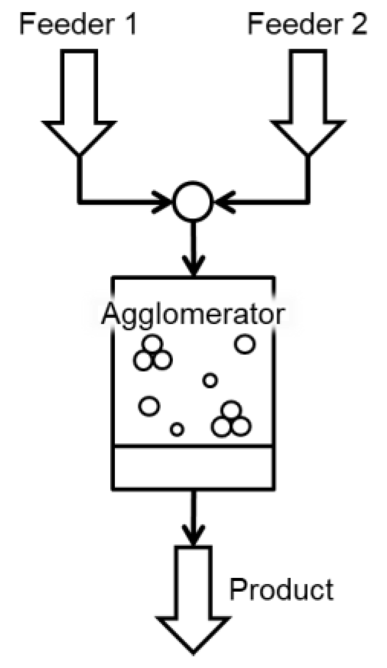
Thus, the use of the method based on transformation matrices is an option for simulation systems with an unlimited number of distributions, since it allows treating all variables correctly, regardless of the number and type of defined distributed parameters. In this case, the model functions are used not directly, but to derive the laws θ of material transition between all classes:
{ T H ( t ) = θ H [ F H ( t ) ] T Y ( t ) = θ Y [ F Y ( t ) ] ,
where T is the transformation matrix.
Define { I N } as a set of indices to address any value in the N -dimensional space, so that
{ I N } = i 1 i 2 i N , i d [ 1 : L d ] , d [ 1 : N ] .
The dimension of the transformation matrix T is twice the number of input dimensions taken into account. Each element T { I N } , { J N } of T denotes a fraction of material moving from the { I N } –th cell of the input distribution to the { J N } –th cell of the output distribution. The output values are obtained by applying the transformation matrix to the corresponding input. For example, for a dynamic unit, at each time step, the holdup is calculated as the transformation of the previous state of the unit while considering the inlet and the outlet streams. The output, in turn, is calculated by applying the transformation laws to the holdup. Accordingly, Equation (5) takes the form
{ H ( t + Δ t ) = T H ( t + Δ t )     H ( t ) Y ( t + Δ t ) = T Y ( t + Δ t )     H ( t + Δ t ) { T H } , { T Y } R M { H } , { Y } R N ,
where denotes the operation of applying the transformation laws. Due to the method of calculating and applying the transformation matrix, this method provides the correct conversion between the N – and M –parameter spaces.
Application of transformation laws for steady-state units is a direct transformation of input variables into output variables, so Equation (6) becomes
Y ( t ) = T Y ( t )     X ( t ) { T Y } R M { Y } R N .
Consider the steady-state case (13) with any X { X ( t ) } and Y { Y ( t ) } . For a simple 1D case with N =   1 and R M = R N , the operation of applying the transformation matrix can be written as
j 1 [ 1 : L 1 ] : Y j 1 = i 1 = 1 L 1 X i 1 · T i 1 , j 1 .
Then, similarly for the general case with R M = R N :
j 1 [ 1 : L 1 ] , j 2 [ 1 : L 2 ] , , j N [ 1 : L N ] : Y j 1 j 2 j N = i 1 = 1 L 1 i 2 = 1 L 2 i N = 1 L N X i 1 i 2 i N · T i 1 i 2 i N , j 1 j 2 j N
or using Equation (11):
{ J N } : Y { J N } = { I N } X { I N } Δ T { I N } , { J N } .
Then for the case R M R N , Equation (16) becomes the following form:
{ J N } : Y { J N } = { I N } X { I N } · T { I M } , { J M } .
For example, for a three-dimensional case, if N is defined for { L 1 , L 2 , L 3   } and M is defined for { L 2 } , Equation (17) can be written as
j 1 [ 1 : L 1 ] , j 2 [ 1 : L 2 ] , j 3 [ 1 : L 3 ] : Y j 1 j 2 j 3 = i 1 = 1 L 1 i 2 = 1 L 2 i 3 = 1 L 3 X i 1 i 2 i 3 · T i 2 , j 2 .
In this way, the transformation matrix calculated for the M -dimensional unit can be applied to calculate the N -dimensional output from the N -dimensional input, even if R M R N . Equations (14)–(18) can be similarly derived for dynamic units (Equation (12)).
Usually, models in solids processing technology are described using equations that directly compute output distributions. Therefore, obtaining the transformation laws θ (Equation (10)) is an additional and nontrivial task that may require significant reformulations of existing models. This paper shows how this can be accomplished for agglomeration and breakage processes.

2.2. Agglomeration

The finite volume method developed by Kumar et al. [44] is used to get the discretized form of the pure agglomeration population balance equation. Taking S ( x ) = 0 and b ( x , y ) = 0 in Equation (1), the general agglomeration PBE for batch process can be written as
u ( x , t ) t = 1 2 0 x β ( x , x x ) u ( x , t ) u ( x x , t ) d x 0 β ( x , x ) u ( x , t ) u ( x , t ) d x
with initial data u ( x , 0 ) = u 0 ( x ) 0 .
Take the whole domain as [ 0 , R ] . Divide the domain into L 1 cells with boundaries x i 1 2 and x i + 1 2 for i = 1 ,   2 , , L 1 where x 1 2 = 0 and x L 1 + 1 2 = R . Take the representative of the i –th cell [ x i 1 2 ,   x i + 1 2 ] as x i = ( x i + 1 2 + x i 1 2 2 ) and cell length Δ x i = x i + 1 2 x i 1 2 .
Define the initial approximation u 0 ( x ) as
u ( 0 , x ) = 1 Δ x i x i 1 2 x i + 1 2 u 0 ( x ) d x .
To get the discretized form of the agglomeration Equation (19), calculate the total birth and death in each cell. For that, collect all those particles from the lower cell which is going to a particular higher cell. This is done by defining some set of indices. Here, the index set is calculated as follows
I i = { ( j , k ) L 1 × L 1 : x i 1 2 < ( x j + x k ) x i + 1 2 } .
Integrating Equation (19) over each cell [ x i 1 2 ,   x i + 1 2 ] , and introducing weights as given by Kumar et al. [44], the discretized form can be obtained
d u i d t = 1 2 ( j , k ) I i β j k u j u k Δ x j Δ x k Δ x i w j k b j = 1 L 1 β i j u i u j Δ x j w i j d .
where w j k b and w i j d are the weights responsible for preservation of number and conservation of mass, respectively. These weights are defined as
w j k b = { x j + x k 2 x l j k ( x j + x k ) , x j + x k R 0 , x j + x k > R
and
w i j d = { x l i j 2 x l i j ( x i + x j ) , x i + x j R 0 , x i + x j > R .
Here l i j is the symmetric index of the cell, where the agglomerate particle ( x i + x j ) falls. Rewrite Equation (22) as
d Δ x i u i d t = 1 2 ( j , k ) I i β j k u j u k Δ x j Δ x k w j k b j = 1 L 1 β i j u i u j Δ x i Δ x j w i j d .
Take g i = Δ x i u i , then Equation (25) gives
d g i d t = 1 2 ( j , k ) I i β j k g j g k w j k b j = 1 L 1 β i j g i g j w i j d .
To get the particle number at some certain time point τ , the time span [ 0 , τ ] is divided into K subintervals [ t , t + Δ t ] , where t 1 = 0 , t K = τ and Δ t is the time step.
Now the particle number g ( t + Δ t ) at time point t + Δ t using transformation matrix T ( t , Δ t ) is given by
g ( t + Δ t ) = g ( t ) · T ( t , Δ t ) .
Here g ( t ) is a 1 × L 1 row matrix with i -th element g i ( t ) , i = 1 , 2 , 3 , , L 1 at time t , and T ( t , Δ t ) is a L 1 × L 1 transformation matrix, calculated at time t to obtain the distribution after time step Δ t . The elements of the transformation matrix are given by
T i j ( t , Δ t ) = { 1 + ( 1 2 ( i , k ) I i β i k g k ( t ) w i k b j = 1 L 1 β i j g j ( t ) w i j d ) Δ t , i = j 1 2 ( i , k ) I i β i k g k ( t ) w i k b Δ t , i < j 0 , i > j .
To improve the accuracy of the scheme (27), the Runge–Kutta method is proposed:
g ( t + Δ t ) = g ( t ) · T ˜ ( t , Δ t )
where
T ˜ ( t , Δ t ) = [ T ( t , Δ t )   · T ( t + Δ t , Δ t 2 ) + ( I T ( t , Δ t 2 ) ) ] .
Here I is the identity matrix. The method given by Equations (29) and (30) gives the second order accuracy.
Since the scheme is explicit, there would be some restriction on the time step to get a non-negative solution of the scheme (Equation (29)). Therefore, the Courant-Friedrichs-Lewy (CFL) condition [46] on the time step is given by
Δ t min i | 2 g i ( t ) Q ( t ) | ,
where
Q ( t ) = W 1 ( g ( t ) ) W 2 ( g ( t ) ) + W 1 ( g * ( t ) ) W 2 ( g * ( t ) ) , W 1 ( g ( t ) ) = 1 2 ( j , k ) I i β j k g j ( t ) g k ( t ) w j k b , W 2 ( g ( t ) ) = j = 1 L 1 β i j g i ( t ) g j ( t ) w i j d , g i * ( t ) = g i ( t ) + Δ t · W 1 ( g ( t ) ) W 2 ( g ( t ) )

2.3. Breakage

To get the equation for the pure breakage, put β ( x , x ' ) = 0 in Equation (1). Hence, the breakage process can be written as the following linear differential equation
u ( x , t ) t = x b ( x , y ) S ( y ) u ( y , t ) d y S ( x ) u ( x , t ) .
So, integrating Equation (33) over the cell [ x i 1 2 ,   x i + 1 2 ] , can be obtained
d u i d t = B i D i ,
where
B i = 1 Δ x i x i 1 2 x i + 1 2 x x L 1 + 1 2 b ( x , ϵ ) S ( ϵ ) u ( ϵ , t ) d ϵ d x
and
D i = 1 Δ x i x i 1 2 x i + 1 2 S ( x ) u ( x , t ) d x ,
where L 1 is the number of discrete size classes.
Take the approximation of the initial data as
u ( x , 0 ) = 1 Δ x i x i 1 2 x i + 1 2 u 0 ( x ) d x .
Proceeding in the same way as Kumar et al. [43], the discretized form with two weight functions can be obtained as
d u i d t = 1 Δ x i k = i L 1 φ k b S k u k Δ x k B i k ψ i d S i u i ,
where the weighted parameters for birth and death φ i b and ψ i d are given by
φ i b = x i ( ϑ ( x i ) 1 ) k = 1 i 1 ( x i x k ) B k i
and
ψ i d = φ i b x i k = 1 i x k B k i , i = 2 , 3 , 4 , , L 1 .
Take φ 1 b = 0 , ψ 1 d = 0 and
B i k = x i 1 2 p k i b ( x ,   x k ) d x
with
p k i = { x i , k = i x i + 1 2 , k i
and
ϑ ( x i ) = 0 x i b ( x ,   x i ) d x .
Multiplying Δ x i on both sides of Equation (38), one obtains
d Δ x i u i d t = k = i L 1 φ k b S k u k Δ x k B i k ψ i d S i u i Δ x i .
Take g i = Δ x i u i . Then, Equation (44) can be rewritten as
d g i d t = k = i L 1 φ k b S k g k B i k ψ i d S i g i .
To get the particle number at some certain time point τ , the time span [ 0 , τ ] is divided into K subintervals [ t , t + Δ t ] , where t 1 = 0 , t k = τ and Δ t is the time step.
The particle number g ( t + Δ t ) at time point t + Δ t using transformation matrix T ( t , Δ t ) is given by
g ( t + Δ t ) = g ( t ) · T ( t , Δ t ) ,
where g ( t ) is a 1 × L 1 row matrix (vectors) with elements denoted by g i ( t ) , and T ( t , Δ t ) is a L 1 × L 1 matrix whose elements are denoted by T i j ( t , Δ t ) . The elements of the transformation matrix can be written with the help of the discretized form of Equation (33) as follows
T i j ( t , Δ t ) = { 1 + ( φ i b B i i ψ i d ) S i Δ t , i = j S i B j i φ i b Δ t , i > j 0 , i < j .
The scheme (Equation (46)) gives the first-order accuracy. To get a higher order accuracy,
g ( t + Δ t ) = g ( t ) · T ˜ ( t , Δ t ) ,
is proposed using the Runge–Kutta method. Here
T ˜ ( t , Δ t ) = [ T ( t , Δ t )   · T ( t + Δ t , Δ t 2 ) + ( I T ( t , Δ t 2 ) ) ] .
I is the identity matrix. The method given by Equations (48) and (49) gives the second order accuracy.
Consider a positive initial data g i ( 0 ) for all i . However, the solution g i ( t ) may become negative. In order to ensure positivity, a condition for the time step must be defined:
Δ t min i | 2 g i ( t ) Q ( t ) | ,
where
Q ( t ) = W 1 ( g ( t ) ) W 2 ( g ( t ) ) + W 1 ( g * ( t ) ) W 2 ( g * ( t ) ) , W 1 ( g ( t ) ) = k = i L 1 φ k b S k g k ( t ) B i k ψ i d S i g i ( t ) , W 2 ( g ( t ) ) = ψ i d S i g i ( t ) , g i * ( t ) = g i ( t ) + Δ t · W 1 ( g ( t ) ) W 2 ( g ( t ) ) .

3. Implementation Details

3.1. Dynamic Flowsheet Simulation in Dyssol

In this work, the Dyssol modelling framework [7] was used to perform simulations using the newly proposed methods. The system is being developed within the priority program of the German Research Foundation (DFG) SPP 1679 “Dynamic simulation of interconnected solids processes DYNSIM-FP” [47].
Dyssol is written entirely in the C++ programming language [48] using a modular architecture and an object-oriented approach [49]. This made it possible to split the entire program into separate, relatively independent modules, to facilitate their development. They are integrated into a single system using specially designed software interfaces. In particular, each model (e.g. agglomerator, mill, or screen) is an independent software library that can be created separately, and then connected to the simulation program. This greatly increases the flexibility and the extensibility of the entire system and simplifies its development and maintenance.
Due to the mathematical complexity and diversity of models in the area of solids processing technology, the calculations in Dyssol are carried out according to the sequential-modular approach [50]. Each model is calculated independently of the others, using its own most appropriate equations solvers and computational methods. The task of the simulation system itself in this case is to manage the information and material flows between the models in accordance with the flowsheet structure and to ensure convergence. The sequential-modular approach simplifies the development of new models, since they are less limited to the implementation and functionality of the modelling framework. Moreover, this method can be effectively applied even at the scale of individual process units [51].
Application of the modular approach imposes some restrictions on the flowsheet structures. In particular, schemes containing recycle flows cannot be calculated directly and require additional treatment. Before starting the simulation, all such flows must be identified and initialized with some predefined values in order to break the cycles [52]. After that, all units inside the recycle loop are calculated iteratively until convergence. To speed up this process, the initial parameters of recycles are calculated anew at each iteration using convergence methods [7,53].
Reaching convergence over a relatively large time interval can be very difficult and can become a resource-intensive task. To overcome this problem, dynamic modelling of flowsheets with recycle flows is performed using an approach based on the waveform relaxation method [54]. Here, iterative calculations are performed only for a certain short time interval [6,15], where convergence can be reached much faster. When the calculation of the current time interval is completed, the system uses data interpolation methods [7] to initialize the next time window and proceeds to its calculation.

3.2. Application of Transformation Matrices

From a mathematical point of view, the application of a full transformation matrix (Equation (16)) is a relatively simple operation and can be described as the regular multiplication of matrices. However, with a large number of matrix dimensions and a large number of classes, such a naive calculation will be very demanding in terms of computational capabilities and memory consumption. Moreover, the need to work with time-dependent parameters imposes additional restrictions on data structures. Therefore, all distributed parameters in Dyssol are stored in sparse format, represented by specially developed tree data structures [7], as is schematically shown in Figure 2 for a single time point.
Here, each hierarchy level describes the distribution of material over a specific parameter, and each entry is the mass fraction of material that has a specific combination of parameters. Since distributions often contain a lot of zero values, such a structure can drastically reduce the amount of data, which needs to be stored and processed. In addition, this data structure allows the use of relative mass fractions for each level of the hierarchy, instead of operating with absolute mass fractions. Thus, from Figure 2 it follows that there are 30% of particles with a size of (2 mm3 + 3 mm3)/2 = 2.5 mm3; of these, 50% have a sphericity of (0.5 + 0.75)/2 = 0.625; and from them, 20% have a porosity of (0.33 + 0.66)/2 = 0.5. The total percentage of particles with this combination of parameters is 0.3 × 0.5 × 0.2 = 3%.
The use of absolute mass fractions and tree structures allows for working with individual distributions without changing information in the others. So, transformation matrices can be effectively applied for each level separately and this will not affect all distributions located at higher hierarchical levels.
Take the N –dimensional distribution represented by N hierarchy levels, where L d is the number of classes in d –th dimension and X q p and Y q p are relative mass fractions in the q –th class of the p –th level in the initial and the transformed distribution, respectively (Figure 3).
If the transformation matrix T is calculated for M –dimensional parameter space, its application will consist of three stages:
  • Apply T to the lowest M –th hierarchy level of input distribution, using Equation (17) in the form of
    Y j 1 j 2 j M 1 j M M = i 1 = 1 L 1 i 2 = 1 L 2 i M 1 = 1 L M 1 i M = 1 L M X i 1 i 2 i M M · X i 1 i 2 i M 1 M 1 · · X i 1 i 2 2 · X i 1 1 · T i 1 i 2 i M , j 1 j 2 j M .
    For example, for M = 2 , the second level of the hierarchy should be calculated as
    Y j 1 j 2 2 = i 1 = 1 L 1 i 2 = 1 L 1 X i 1 i 2 2 · X i 1 1 · T i 1 i 2 , j 1 j 2
  • Extract the transformation laws for the previous level ( M 1 ) from T and apply them using Equation (52). Repeat it up to the hierarchy level 1. For example, for M = 2 , the first level will be calculated as
    Y j 1 1 = i 1 = 1 L 1 X i 1 1 · T i 1 , j 1 ,
    which corresponds to Equation (14).
  • Apply T to calculate the remaining levels K below M as
    Y j 1 j 2 j K 1 j K K = i 1 = 1 L 1 X i 1 j 2 j K K · X i 1 j 2 j K 1 K 1 · · X i 1 j 2 2 · X i 1 1 · T i 1 , j 1 Y j 1 j 2 j K 1 K 1 · Y j 1 j 2 j K 2 K 2 · · Y j 1 j 2 2 · Y j 1 1 , M < K N
    For example, if M = 1 and K = 2 :
    Y j 1 j 2 2 = i 1 = 1 L 1 X i 1 j 2 2 · X i 1 1 · T i 1 , j 1 Y j 1 1 .
Thus, using Equations (52) and (55), as well as sorting the levels in the hierarchical data structure, one can apply the transformation matrix of any complexity to any input distribution.
Depending on the unit type, the conventional algorithm for applying transformation matrices varies:
  • For steady state units: copy the distribution from the input to the output, then apply the transformation matrix to the output.
  • For dynamic units: use the input distribution to calculate the holdup, apply the transformation matrix to the holdup, and then calculate the output.
In the latter case, because of time discretization, the mixing of the input material with the holdup and the application of the transformation matrix are performed sequentially.

3.3. Implementation of Units

To verify and investigate the proposed new methods, the Dyssol simulation system has been extended with several models that have been implemented using the provided program interfaces.

3.3.1. Agglomerator

The new method of solving the agglomeration PBE was implemented as a new model of the Dyssol simulation system according to Equation (29). To simplify the model, it was assumed that the mass within the apparatus remains constant and there is no classification by size at the output. Therefore, the mass flow of material leaving the apparatus m ˙ o u t ( t ) equals to the mass flow entering it m ˙ i n ( t ) , and the distribution of the material at the output Y ( t ) equals to the distribution in the holdup H ( t ) .
Since the applicability of the proposed method does not depend on the chosen agglomeration kernel, to describe the agglomeration rate in all case studies, a frequently used physically relevant kernel based on a Brownian motion [55,56] was applied in the following from:
β ( x , x ) = β 0 β * ( x 1 3 + x 1 3 ) ( x 1 3 + x 1 3 ) , β * = { 1 , x + x x a , m i n   1 ( x + x ) x a , m i n x a , m a x x a , m i n , x a , m i n < x + x < x a , m a x 0 , x + x x a , m a x .
Here β ( x , x ) denotes the agglomeration rate between particles x and x ; β 0 is the size-independent agglomeration rate constant, dependent on operating conditions; β * is the size- dependent agglomeration rate constant; and x a , m i n and x a , m a x are minimum and maximum sizes of resulting agglomerates.
The agglomerator unit was implemented according to Equations (28) and (29) to calculate and apply the transformation matrix for the particles size. To consider secondary distributions, it was extended to perform aggregation with averaging of the properties distributed over the second dimension, which is calculated as follows.
Let particles of two sizes x s r c 1 and x s r c 2 aggregate into a particle of size x d s t . Then T s r c 1 , d s t and T s r c 2 , d s t are the corresponding entries of the transformation matrix, calculated by Equation (28). The summarized mass fraction of particles from size-class i is distributed over L 2 classes of the secondary dimension, so that
c i = j = 1 L 2 c i , j ,
where c i , j is a mass fraction of granular material with size x i and value of the secondary dimension falling into class j . If particles from two classes ( s r c 1 , j 1 ) and ( s r c 2 , j 2 ) aggregate, the result lands into some class ( d s t , j ) . The size-class d s t is directly determined from the agglomeration mechanism and obtained from the transformation matrix. The mass fraction of each j –th class of the secondary distribution is calculated as
c d s t , j = j 1 = 1 L 2 j 2 = 1 L 2 ( c s r c 1 , j 1 T s r c 1 , d s t ) · ( c s r c 2 , j 2 · T s r c 2 , d s t ) k = 1 S 2 c s r c 2 , k · T s r c 2 , d s t
whereas the class index j for equidistant grid can be obtained as
j = j 1 · c s r c 1 , j 1 · T s r c 1 , d s t + j 2 · c s r c 2 , j 2 · T s r c 2 , d s t c s r c 1 , j 1 · T s r c 1 , d s t + c s r c 2 , j 2 · T s r c 2 , d s t .

3.3.2. Mill

The mill model, developed in Dyssol, implements Equations (47) and (48) to calculate transformation laws and Equations (52) and (55) to apply them. To calculate Equations (41) and (43), the adaptive Simpson’s method of numerical integration [57] was applied. The criterion used to determine when to terminate interval subdivision was chosen according to Lyness [58], and its desired tolerance was set to 10−15.
For simplification, the holdup mass within the unit stays constant and no classification by size occurs at the outlet.
As can be seen from Section 2.3, the proposed approach does not depend on the chosen selection or breakage functions. Therefore, for testing purposes, the following physically relevant models were taken from literature. To describe the selection rate in all case studies, the selection function based on the model proposed by King [59] was applied:
S ( x ) = s 0 · { 0 ,   x x b , m i n 1 ( x b , m a x   x x b , m a x   x b , m i n ) n , x b , m i n < x < x b , m a x 1 , x x b , m a x ,
where S ( x ) is the mass fraction of particles of size x that are crushed; s 0 introduces a size-independent selection rate factor; x b , m i n and x b , m a x are critical sizes of particles; and n is a power law exponent of the King’s selection function.
The breakage function was implemented according to Vogel et al. [60] in a number-based distributed form:
B ( x , y ) = { 0.5 q y ( x y ) q 2 ( 1 + t a n h ( y y ' y ' ) ) , y x 0 , y < x .
Here B ( x , y ) denotes the mass fraction of particles with the size of y , which after breakage get the size less or equal to x ; y ' is the minimum fragment size that can be achieved after milling; and q is a power law exponent of the Vogel breakage function.

3.3.3. Screen

The screen apparatus is a steady-state unit, which is described in terms of the grade efficiency G ( x ) , calculated according to the model of Plitt [61] as
G ( x ) = 1 e x p ( 0.693 ( x x c u t ) α ) .
G ( x ) determines the mass fraction of material of size x , which leaves the screen through an outlet for coarse particles; x c u t is the cut size of the classification model; α is the separation sharpness.
For proper consideration of the distributed parameters, each deck of the screen unit formulates two diagonal transformation matrices for the particle size distribution (PSD): for coarse ( T c ) and for fines ( T f ) output, so that
T i , i c = G ( x i ) T i , i f = 1 G ( x i ) .
The total mass flows of coarse m ˙ o u t c and fines m ˙ o u t f outlets can be calculated as
m ˙ o u t c = m ˙ i n i = 1 L 1 G ( x i ) · c i m ˙ o u t f = m ˙ i n ( 1 i = 1 L 1 G ( x i ) · c i ) ,
where m ˙ i n is the mass flow at the inlet, c i is the mass fraction of particles of size x i , and L 1 is the number of size classes.
Application of the transformation matrices was performed according to Equations (52) and (55).

4. Simulation Examples
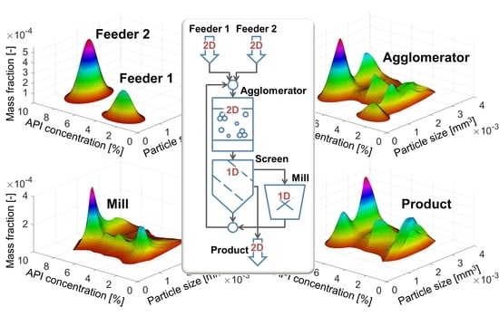
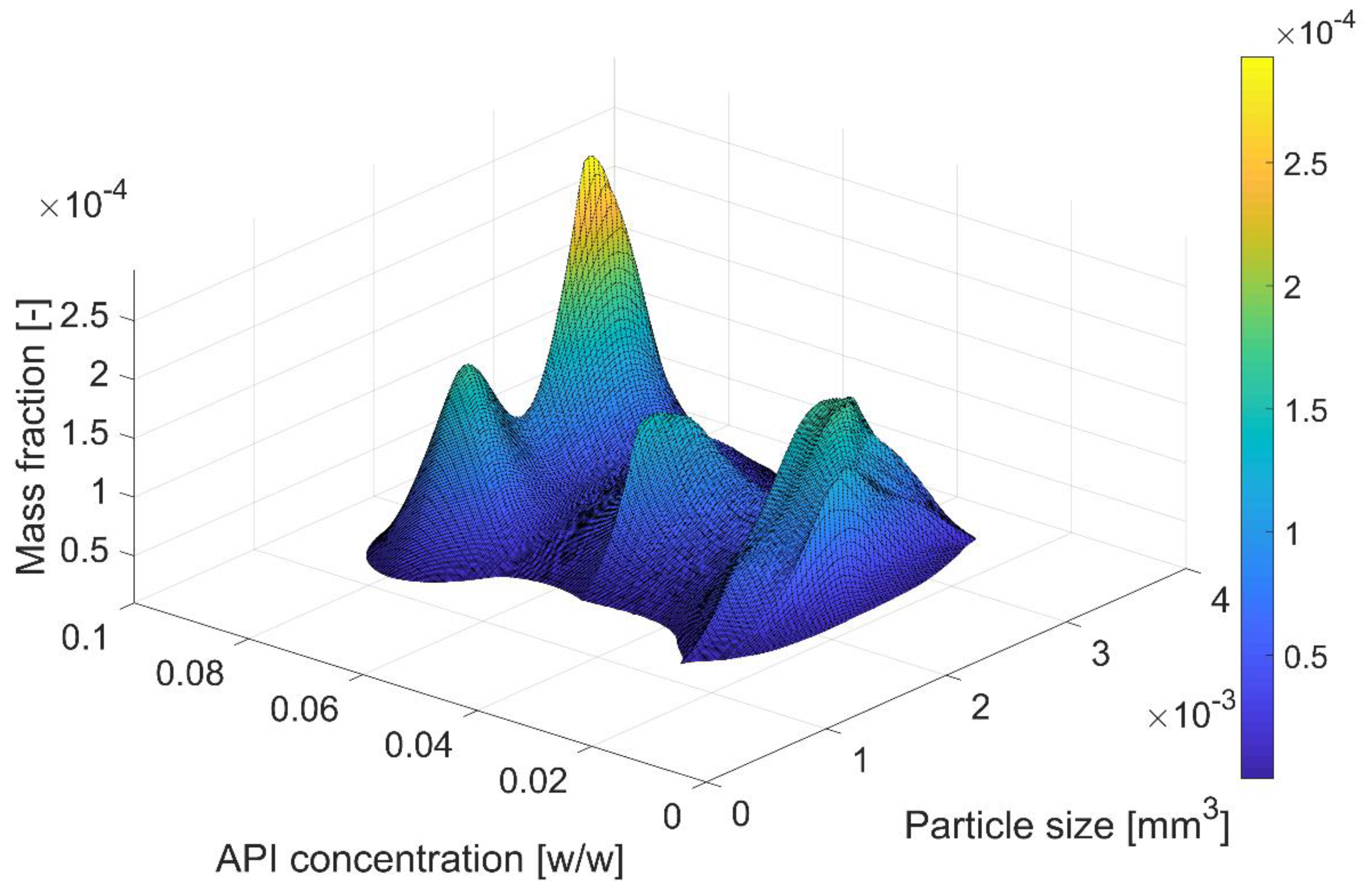
All simulations were performed in the dynamic flowsheet simulation system Dyssol using the developed models, described in Section 3.3.

4.1. Agglomeration

A simple pharmaceutical process of agglomerating blends with two different concentrations of the active pharmaceutical ingredient (API) was simulated. The process structure is illustrated in Figure 4. The solid material is described using two interdependent distributed parameters:
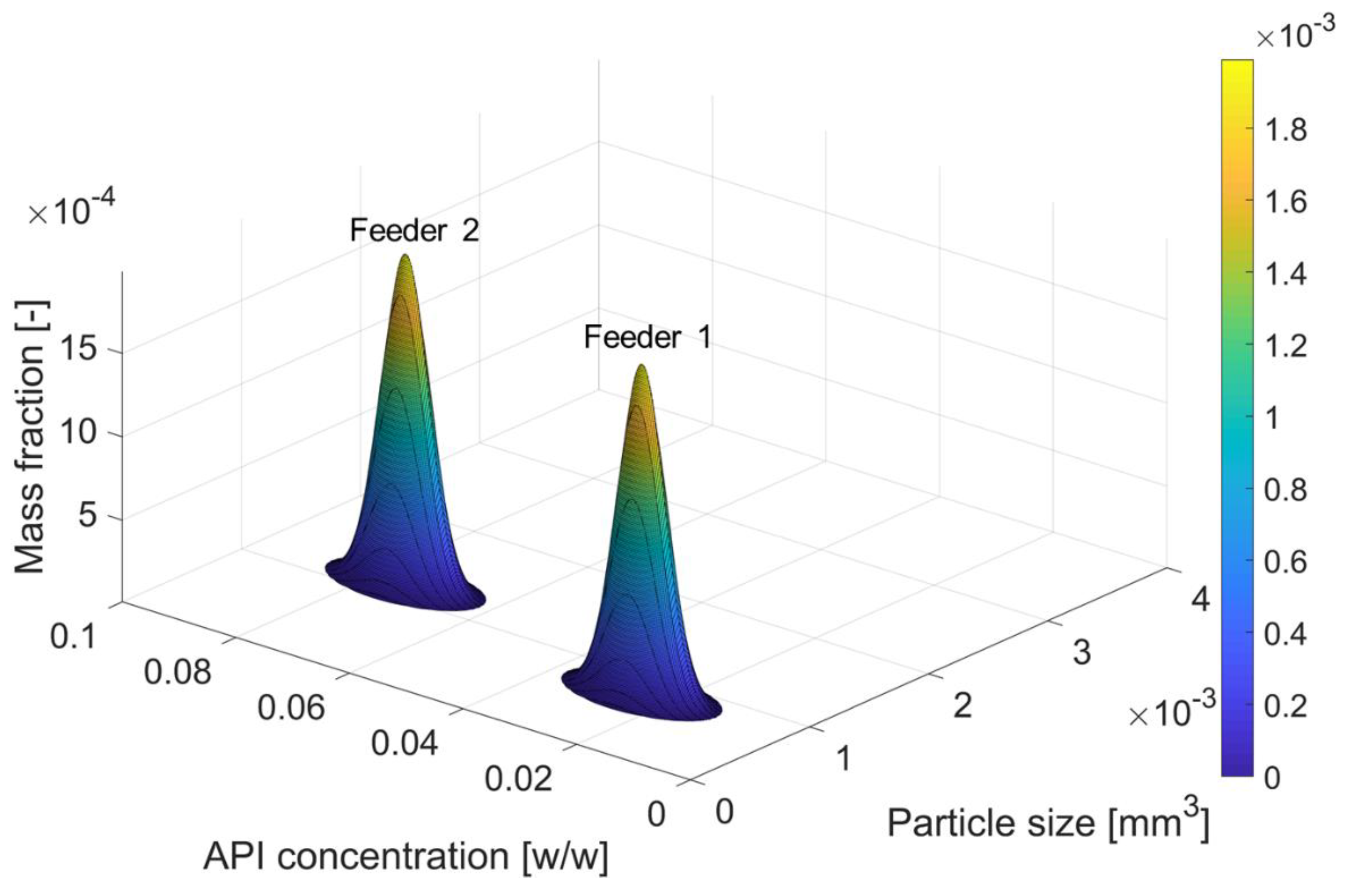
  • Particle size representing the volume of particles ranging from 0 to 4 × 10⁻³ mm3 and distributed over 100 equidistant classes; and
  • the API concentration, which describes the mass content of an active ingredient from 0 to 10% divided into 500 equidistant classes.
The initial blend entering the agglomerator is a mixture of materials from two feeders (Figure 5):
  • Feeder 1 supplies smaller particles with a lower API concentration;
  • Feeder 2 supplies larger particles with a higher API concentration.
Both particle sizes and API concentrations are given in terms of the Gaussian normal distribution with mean values μ and standard deviations σ shown in Table 1. Feeders continuously supply the material at a rate of 0.25 kg/s each. The final distribution after their mixing is shown in Figure 5. The agglomerator is initially filled with 200 kg of the same blend. All model parameters used to simulate the agglomeration process are listed in Table 1.
Figure 6 and Figure 7 show the distribution of the product stream in steady-state, which was reached after 25 min of process time. Clearly visible individual peaks, which were formed as a result of the agglomeration of particles with different sizes and different API concentrations. Since the initial blend is supplied continuously at a constant rate during the entire agglomeration process, the initial distributions A and B (Figure 7) are still distinguishable in the final mixture. Agglomeration of material B with itself gives F, which has a doubled mean size and the same API concentration as B, as expected. In turn, agglomeration of B with F (having the same concentrations) gives a peak at M, which does not alter API content and has a particle size equal to (B + F). The same is true for the material from feeder 1, agglomerating with itself according to the schema: (A + A) = C, (A + C) = E, and (A + E) + (C + C) = H.
More complex behaviour is observed if particles with different API concentrations agglomerate. In this case, the particle sizes are added up and the concentration is averaged according to Equation (59). For example, agglomeration of particles from A and B gives D. Further, G is formed as a mixture of (A + D) and (B + C). The result of the agglomeration of B and C is shifted below the concentration value of 0.05 due to the mutual influence of two factors. First, the introduction of the size-dependent growth rate β * (Equation (57)) leads to faster growth of smaller particles. Second, averaging by the second distribution takes into account the actual amount of material being agglomerated in selected classes (see Equations (59) and (60)).
The complete scheme of material transitions during the agglomeration, shown in Figure 7, is represented in Table 2.
Thus, information on the change in particle size during the agglomeration process, obtained from the generated transformation matrix, made it possible to take into account and correctly process the dependent distributed parameters of the agglomerated material.

4.2. Breakage

To verify the proposed new method for solving the breakage PBE, a simplified process of milling a two-component blend was simulated. Figure 8 shows its flowsheet structure. Two feeders supply material with different particle sizes and API concentrations into the system. Their mixture, shown in Figure 9, enters the mill unit to be mixed with the holdup material and crushed afterwards.
The initial blend entering mill is a mixture of smaller particles with a higher API concentration and larger particles with a lower API concentration. Both distributed parameters are given as Gaussian normal distributions with parameters from Table 3. The mill is initially filled with 50 kg of the same blend (Figure 9).
The particle size is described between 0 to 4 × 10⁻³ mm3 with 100 equidistant classes, whereas the mass content of an active ingredient is distributed over 500 equidistant classes ranging from 0 to 10%.
All model parameters used to simulate breakage process are listed in Table 3.
The steady-state is reached in 25 min of the process time. Figure 10 and Figure 11 show the distribution of the product after this time point.
Due to the constant supply of material during the whole process time, initial distributions A and B (Figure 11) are still clearly visible in the product. At the same time, it is evident from Figure 10 that the reduction in particle size caused by the breakage process does not lead to changes in the content of the active component: the distribution of the API concentration in the outlet stream remains the same as in the initial distribution. Both A and B do not mix, but only change particle size gradually grinding down from A to C and from B to D.
Thus, with the help of transformation matrices, it was possible to avoid mixing the secondary parameters, despite the fact that the model of the mill unit was developed considering only the particle size distribution.

4.3. Coupled Agglomeration and Breakage

Having both models of agglomerator and mill, it is possible to simulate part of a complex pharmaceutical process with a closed circuit and an external classification of the material, as it is shown in Figure 12. New material enters the process through two feeders, supplying particles with different sizes and concentrations of API, which mixture is shown in Figure 13. This blend is mixed with the holdup inside the agglomerator, where the growth of particles occurs. The two-compartment screen unit separates material leaving the agglomerator into three fractions. Oversized particles are crushed using the mill unit, and afterwards combined with the undersized particles and sent back to the agglomerator by mixing with external material from feeders. The middle-sized agglomerates are considered as product. Initially, both agglomerator and mill are filled with the same material as it comes from feeder 1.
All model parameters used to simulate the process from Figure 12 can be found in Table 4. Initial distributions of material are given by Gaussian function.
The flowsheet was simulated until a steady state was reached, which occurred after 40 min of the process time. The distribution of the product is shown in Figure 14. There are two peaks for particles with a higher API concentration. One is mainly due to the presence of the source blend from feeder 2 (its coarse part obtained after the sieving), mixed with new particles formed in agglomerator and mill. The second peak is the result of agglomeration of particles with the same high API concentration with each other. For a low API content, only one peak is observed, since all smaller fractions (from agglomeration of the primary material from feeder 1 and milling results) were cut off by the screen unit. At the same time, a mixture of two initial blends, formed as a result of the agglomeration of materials with different API content, is present in a significant amount, but does not dominate the material with initial concentrations.
In general, using the description of granular materials with multidimensional distributions and units developed on the basis of transformation matrices, it is possible to perform simulations of complex processes involving materials distributed over a large number of dimensions. Thus, in this example, it is possible to assess the homogeneity of the material that appears at the output of the simulated process, since this parameter is crucial in pharmaceutical production.

5. Conclusions

The use of transformation matrices is a prerequisite for working with multidimensional distributed parameters of solids. This approach allows for proper handling of all parameters of granular materials, even those which are not directly handled by the model. Consequently, the number of distributed parameters in the model and in its environment may not match. At the same time, the development of each individual model becomes more complicated due to the fact that in contrast to the traditional approach, when the output distribution is explicitly calculated and set to the outlet, it is required to derive the laws of material transformation between inputs and outputs for each time step.
In this article, the applicability of transformation matrices to the description of processes of agglomeration and crushing, which are usually formulated by the population balance equations, was shown. The proposed new methods allow for extracting information about the transformation laws from PBEs and calculating the transformation matrices on that basis. The approach uses the finite volume method for spatial discretization and the second-order Runge–Kutta method for obtaining the complete discretized form of the population balance equations.
To perform the test studies, the derived methods have been implemented in the dynamic flowsheet simulation environment Dyssol. Some exemplary production processes and their parts were simulated using the derived models to prove the applicability and advantages of presented approaches for modelling of granular materials described by multidimensional distributed parameters.
As case studies have shown, the use of transformation matrices enables the correct calculation of the dependent secondary parameters, avoiding their mixing during the simulation. The proposed method can be extended with additional laws for dependent parameters, for example, for mixing of materials. This will significantly expand its application scope and will allow simulating more sophisticated processes. In general, the proposed approach allows usage of a more complex description of materials with the help of several distributed parameters, without the need to adjust each specific model, and transferring the task of their correct calculation to the modelling system. In this way, the new method of reformulating population balance equations greatly increases the possibilities for creating generally applicable systems for the simulation of solid phase processes.

Author Contributions

Conceptualization: M.D. and J.K.; methodology: M.D., N.D., and V.S.; software: V.S.; validation: V.S. and N.D.; formal analysis: V.S.; investigation: V.S. and N.D; data curation: V.S.; writing—original draft preparation: V.S. and N.D.; writing—review and editing: V.S., N.D., M.D., S.H., and J.K.; visualization: V.S.; supervision: S.H., J.K., and M.D.; project administration: M.D.; funding acquisition: S.H., M.D., and J.K.

Funding

Authors gratefully acknowledge the financial support of the Deutsche Forschungsgemeinschaft (DFG, German Research Foundation) within the priority program SPP 1679 “Dynamic simulation of interconnected solids processes DYNSIM-FP”; of the German Academic Exchange Service (DAAD) via Research Grants—Bi-nationally Supervised Doctoral Degrees, 2017/18 (57299293); of the Alexander von Humboldt Foundation (Research Group Linkage Programme); and of the DFG—Projektnummer 392323616 and the Hamburg University of Technology (TUHH) via the funding programme “Open Access Publishing”.

Conflicts of Interest

The authors declare no conflict of interest.

Notation

b ( x : y ) fraction of particles of size x formed due to the breakage of a particle of size y  
  b i j   fraction of particles of size-class i formed due to the breakage of a particle of size-class j  
  c   control variables of a unit
  c i , j   mass fraction of granular material falling into class ( i , j ) of two-dimensional distribution
  d   index of a distributed property
  F H , F Y   model functions of a unit for calculating holdup and output, respectively
  G   grade efficiency of the screen unit
  H   unit’s holdup variables
  I   identity matrix
  L   total number of discrete classes for all distributed properties
  L d   number of discrete classes for distributed property d  
  m ˙ i n , m ˙ o u t   mass flow at the inlet and at the outlet streams of a unit, respectively
  M   number of distributed properties in a model
  n   power law exponent of the King’s selection function
  N   number of distributed properties in a flowsheet
  p   model parameters of a unit
  q   power law exponent of the Vogel breakage function
  Q ˙ i n , Q ˙ o u t   distribution of particles by size at the input and at the output of a unit, respectively
  r   design or structural parameters of a unit
  R   maximum size of particles in the considered interval
  R N   parameter space formed by N distributed parameters
  s 0   size-independent selection rate factor
  S ( y )   breakage rate of a particle of size y  
  S i   breakage rate of a particle from size-class i  
  t   time
  T ( t , Δ t )   transformation matrix, calculated at time t to obtain the distribution after time step Δ t  
  T i j   particular entry of a transformation matrix with specific indices
  T H , T Y   transformation matrices to calculate holdups and output of a unit, respectively
  u ( x )   mass fraction of particles of size x  
  u 0 ( x )   mass fraction of particles of size x at the initial moment of time
  u i   mass fraction of particles from size-class i  
  w b , w d   weighting parameters for agglomeration, for birth and death of particles, respectively
  x , x   particle sizes
  x a , m i n   , x a , m a x   critical sizes of particles for agglomeration
  x b , m i n , x b , m a x   critical sizes of particles for breakage
  x c u t   cut size of the screen unit
  x i   size of particles in a discrete class i  
  X   unit’s input variables
  X q p   relative mass fraction, stored in the q –th class of the p –th hierarchical level in the initial distribution
  y   particle size
  y   minimum fragment size of the Vogel breakage function
  Y   unit’s output variables
  Y q p   relative mass fraction, stored in the q –th class of the p –th hierarchical level in the transformed distribution
  α   separation sharpness of the screen unit
  β ( x , x )   agglomeration rate for particles of sizes x and x  
  β i j   agglomeration rate for particles from size-classes i and j  
  β 0   size-independent agglomeration rate constant
  β *   size-dependent agglomeration rate constant
  Δ x i   length of size-class i  
  ϑ ( y )   total number of particles of size y appearing after breakage
  θ H , θ Y   model functions of a unit in terms of the laws of material transition
  μ c o n c   mean value of the normal distribution function describing API concentration
  μ s i z e   mean value of the normal distribution function describing particle sizes
  σ c o n c   standard deviation of the normal distribution function describing API concentration
  σ s i z e   standard deviation of the normal distribution function describing particle sizes
  φ b , ψ d   weighting parameters for breakage, for birth and death of particles, respectively
operation of applying the transformation matrix
  { I N }   set of indices to address any value in the N –dimensional parameter space
  I i   set of indices to address particles going from a lower to a higher cell

References

  1. Kovačević, T.; Wiedmeyer, V.; Schock, J.; Voigt, A.; Pfeiffer, F.; Sundmacher, K.; Briesen, H. Disorientation angle distribution of primary particles in potash alum aggregates. J. Cryst. Growth 2017, 467, 93–106. [Google Scholar] [CrossRef] [Green Version]
  2. Liu, L.X.; Litster, J.D.; Iveson, S.M.; Ennis, B.J. Coalescence of deformable granules in wet granulation processes. AIChE J. 2000, 46, 529–539. [Google Scholar] [CrossRef]
  3. Iveson, S.M.; Beathe, J.A.; Page, N.W. The dynamic strength of partially saturated powder compacts: The effect of liquid properties. Powder Technol. 2002, 127, 149–161. [Google Scholar] [CrossRef]
  4. Alaathar, I.; Hartge, E.-U.; Heinrich, S.; Werther, J. Modeling and flowsheet simulation of continuous fluidized bed dryers. Powder Technol. 2013, 238, 132–141. [Google Scholar] [CrossRef]
  5. Pogodda, M. Development of an Advanced System for the Modeling and Simulation of Solids Processes; Shaker Verlag: Aachen, Germany, 2007. [Google Scholar]
  6. Dosta, M. Dynamic Flowsheet Simulation of Solids Processes and Its Application to Fluidized Bed Spray Granulation; Cuvillier Verlag: Göttingen, Germany, 2013. [Google Scholar]
  7. Skorych, V.; Dosta, M.; Hartge, E.-U.; Heinrich, S. Novel system for dynamic flowsheet simulation of solids processes. Powder Technol. 2017, 314, 665–679. [Google Scholar] [CrossRef]
  8. Hartge, E.U.; Pogodda, M.; Reimers, C.; Schwier, D.; Gruhn, G.; Werther, J. Flowsheet simulation of solids processes. KONA Powder Part. J. 2006, 24, 146–158. [Google Scholar] [CrossRef]
  9. Werther, J.; Heinrich, S.; Dosta, M.; Hartge, E.-U. The ultimate goal of modelling—Simulation of system and plant performance. Particuology 2011, 9, 320–329. [Google Scholar] [CrossRef]
  10. Aspentech—Aspen Plus. Available online: https://www.aspentech.com/en/products/engineering/aspen-plus (accessed on 24 July 2019).
  11. PSE Products—gFORMULATE—gPROMS FormulatedProducts—Solids Processing. Available online: https://www.psenterprise.com/products/gproms/formulatedproducts (accessed on 24 July 2019).
  12. JKSimMet—JKTech Simulation of Comminution and Classification Circuits. Available online: https://jktech.com.au/jksimmet (accessed on 24 July 2019).
  13. HSC Sim—Process Simulation Module. Available online: https://www.outotec.com/products/digital-solutions/hsc-chemistry/hsc-sim-process-simulation-module (accessed on 24 July 2019).
  14. CHEMCAD—Chemical Engineering Simulation Software by Chemstations. Available online: https://www.chemstations.com/CHEMCAD (accessed on 24 July 2019).
  15. Dosta, M.; Heinrich, S.; Werther, J. Fluidized bed spray granulation: Analysis of the system behaviour by means of dynamic flowsheet simulation. Powder Technol. 2010, 204, 71–82. [Google Scholar] [CrossRef]
  16. Neugebauer, C.; Palis, S.; Bück, A.; Diez, E.; Heinrich, S.; Tsotsas, E.; Kienle, A. Influence of mill characteristics on stability of continuous layering granulation with external product classification. Comput. Aided Chem. Eng. 2016, 38, 1275–1280. [Google Scholar]
  17. Haus, J.; Hartge, E.-U.; Heinrich, S.; Werther, J. Dynamic flowsheet simulation for chemical looping combustion of methane. Int. J. Greenh. Gas Control 2018, 72, 26–37. [Google Scholar] [CrossRef]
  18. Koeninger, B.; Hensler, T.; Romeis, S.; Peukert, W.; Wirth, K.-E. Dynamics of fine grinding in a fluidized bed opposed jet mill. Powder Technol. 2018, 327, 346–357. [Google Scholar] [CrossRef]
  19. Sander, S.; Gawor, S.; Fritsching, U. Separating polydisperse particles using electrostatic precipitators with wire and spiked-wire discharge electrode design. Particuology 2018, 38, 10–17. [Google Scholar] [CrossRef]
  20. Boukouvala, F.; Niotis, V.; Ramachandran, R.; Muzzio, F.J.; Ierapetritou, M.G. An integrated approach for dynamic flowsheet modeling and sensitivity analysis of a continuous tablet manufacturing process. Comput. Chem. Eng. 2012, 42, 30–47. [Google Scholar] [CrossRef]
  21. Rogers, A.J.; Inamdar, C.; Ierapetritou, M.G. An integrated approach to simulation of pharmaceutical processes for solid drug manufacture. Ind. Eng. Chem. Res. 2014, 53, 5128–5147. [Google Scholar] [CrossRef]
  22. Skorych, V.; Dosta, M.; Hartge, E.-U.; Heinrich, S.; Ahrens, R.; Le Borne, S. Investigation of an FFT-based solver applied to dynamic flowsheet simulation of agglomeration processes. Adv. Powder Technol. 2019, 30, 555–564. [Google Scholar] [CrossRef]
  23. Sastry, K.V.S. Similarity size distribution of agglomerates during their growth by coalescence in granulation or green pelletization. Int. J. Miner. Process. 1975, 2, 187–203. [Google Scholar] [CrossRef]
  24. Hill, P.J.; Ng, K.M. Statistics of multiple particle breakage. AIChE J. 1996, 42, 1600–1611. [Google Scholar] [CrossRef]
  25. Hulburt, H.M.; Katz, S. Some problems in particle technology: A statistical mechanical formulation. Chem. Eng. Sci. 1964, 19, 555–574. [Google Scholar] [CrossRef]
  26. Barrett, J.; Jheeta, J. Improving the accuracy of the moments method for solving the aerosol general dynamic equation. J. Aerosol Sci. 1996, 27, 1135–1142. [Google Scholar] [CrossRef]
  27. Madras, G.; McCoy, B.J. Reversible crystal growth-dissolution and aggregation-breakage: Numerical and moment solutions for population balance equations. Powder Technol. 2004, 143, 297–307. [Google Scholar] [CrossRef]
  28. Marchisio, D.L.; Fox, R.O. Solution of population balance equations using the direct quadrature method of moments. J. Aerosol Sci. 2005, 36, 43–73. [Google Scholar] [CrossRef]
  29. Kumar, S.; Ramkrishna, D. On the solution of population balance equations by discretization—I. A fixed pivot technique. Chem. Eng. Sci. 1996, 51, 1311–1332. [Google Scholar] [CrossRef]
  30. Vale, H.M.; McKenna, T.F. Solution of the population balance equation for two-component aggregation by an extended fixed pivot technique. Ind. Eng. Chem. Res. 2005, 44, 7885–7891. [Google Scholar] [CrossRef]
  31. Kruis, F.E.; Maisels, A.; Fissan, H. Direct simulation Monte Carlo method for particle coagulation and aggregation. AIChE J. 2000, 46, 1735–1742. [Google Scholar] [CrossRef]
  32. Lee, K.; Matsoukas, T. Simultaneous coagulation and break-up using constant-N Monte Carlo. Powder Technol. 2000, 110, 82–89. [Google Scholar] [CrossRef]
  33. Lin, Y.; Lee, K.; Matsoukas, T. Solution of the population balance equation using constant-number Monte Carlo. Chem. Eng. Sci. 2002, 57, 2241–2252. [Google Scholar] [CrossRef]
  34. Smith, M.; Matsoukas, T. Constant-number Monte Carlo simulation of population balances. Chem. Eng. Sci. 1998, 53, 1777–1786. [Google Scholar] [CrossRef]
  35. Mahoney, A.W.; Ramkrishna, D. Efficient solution of population balance equations with discontinuities by finite elements. Chem. Eng. Sci. 2002, 57, 1107–1119. [Google Scholar] [CrossRef]
  36. Nicmanis, M.; Hounslow, M. A finite element analysis of the steady state population balance equation for particulate systems: Aggregation and growth. Comput. Chem. Eng. 1996, 20, S261–S266. [Google Scholar] [CrossRef]
  37. Rigopoulos, S.; Jones, A.G. Finite-element scheme for solution of the dynamic population balance equation. AIChE J. 2003, 49, 1127–1139. [Google Scholar] [CrossRef]
  38. Hackbusch, W. On the efficient evaluation of coalescence integrals in population balance models. Computing 2006, 78, 145–159. [Google Scholar] [CrossRef]
  39. Le Borne, S.; Shahmuradyan, L.; Sundmacher, K. Fast evaluation of univariate aggregation integrals on equidistant grids. Comput. Chem. Eng. 2015, 74, 115–127. [Google Scholar] [CrossRef]
  40. Matveev, S.A.; Smirnov, A.P.; Tyrtyshnikov, E.E. A fast numerical method for the Cauchy problem for the Smoluchowski equation. J. Comput. Phys. 2015, 282, 23–32. [Google Scholar] [CrossRef]
  41. Kumar, J.; Peglow, M.; Warnecke, G.; Heinrich, S. An efficient numerical technique for solving population balance equation involving aggregation, breakage, growth and nucleation. Powder Technol. 2008, 182, 81–104. [Google Scholar] [CrossRef]
  42. Mostafaei, P.; Rajabi-Hamane, M. Numerical solution of the population balance equation using an efficiently modified cell average technique. Comput. Chem. Eng. 2017, 96, 33–41. [Google Scholar] [CrossRef]
  43. Kumar, J.; Saha, J.; Tsotsas, E. Development and convergence analysis of a finite volume scheme for solving breakage equation. SIAM J. Numer. Anal. 2015, 53, 1672–1689. [Google Scholar] [CrossRef]
  44. Kumar, J.; Kaur, G.; Tsotsas, E. An accurate and efficient discrete formulation of aggregation population balance equation. Kinet. Relat. Models 2016, 9, 373–391. [Google Scholar] [Green Version]
  45. Schwier, D.; Hartge, E.-U.; Werther, J.; Gruhn, G. Global sensitivity analysis in the flowsheet simulation of solids processes. Chem. Eng. Process. 2010, 49, 9–21. [Google Scholar] [CrossRef]
  46. Courant, R.; Friedrichs, K.; Lewy, H. Über die partiellen Differenzengleichungen der mathematischen physik. Math. Ann. 1928, 100, 32–74. [Google Scholar] [CrossRef]
  47. DFG-Priority Programme SPP 1679. Available online: https://www.dynsim-fp.de/en/home (accessed on 24 July 2019).
  48. Stroustrup, B. The C++ Programming Language, 4th ed.; Addison-Wesley: Boston, MA, USA, 2013. [Google Scholar]
  49. Stroustrup, B. Tour of C++, 4th ed.; Addison-Wesley: Boston, MA, USA, 2014; pp. 23–57. [Google Scholar]
  50. Hillestad, M.; Hertzberg, T. Dynamic simulation of chemical engineering systems by the sequential modular approach. Comput. Chem. Eng. 1986, 10, 377–388. [Google Scholar] [CrossRef]
  51. Dosta, M. Modular-based simulation of single process units. Chem. Eng. Technol. 2019, 42, 699–707. [Google Scholar] [CrossRef]
  52. Towler, G.; Sinnott, R. Chemical Engineering Design: Principles, Practice and Economics of Plant and Process Design, 2nd ed.; Butterworth-Heinemann: Kidlington, Oxford, UK, 2013; pp. 223–236. [Google Scholar]
  53. Dimian, A.C.; Bildea, C.S.; Kiss, A.A. Dynamic Simulation. Comput. Aided Chem. Eng. 2014, 35, 127–156. [Google Scholar]
  54. Lelarasmee, E.; Ruehli, A.E.; Sangiovanni-Vincintelli, A.L. The Waveform Relaxation Method for Time-Domain Analysis of Large Scale Integrated Circuits: Theory and Applications. Ph.D. Thesis, University of California, Berkeley, Berkeley, CA, USA, 1982. [Google Scholar]
  55. Smoluchowski, M. Versuch einer mathematischen Theorie der Koagulationskinetik kolloider Losungen. Z. Phys. Chem. 1916, 17, 129–168. [Google Scholar] [CrossRef]
  56. Aldous, D.J. Deterministic and stochastic models for coalescence (aggregation and coagulation): A review of the mean-field theory for probabilists. Bernoulli 1999, 5, 3–48. [Google Scholar] [CrossRef]
  57. Kuncir, G.F. Algorithm 103: Simpson’s rule integrator. Commun. ACM 1962, 5, 347. [Google Scholar] [CrossRef]
  58. Lyness, J.N. Notes on the adaptive Simpson quadrature routine. J. ACM 1969, 16, 483–495. [Google Scholar] [CrossRef]
  59. King, R.P. Modeling and Simulation of Mineral Processing Systems; Butterworth & Heinemann: Oxford, UK, 2001; p. 158. [Google Scholar]
  60. Vogel, L.; Peukert, W. Modelling of grinding in an air classifier mill based on a fundamental material function. KONA Powder Part. J. 2003, 21, 109–120. [Google Scholar] [CrossRef]
  61. Plitt, L.R. The analysis of solid-solid separations in classifiers. CIM Bull. 1971, 64, 42–47. [Google Scholar]
Figure 1. Simplified scheme of embedding a model into a flowsheet.
Processes 07 00535 g001
Figure 2. Tree data structure for storing interdependent multidimensional distributed parameters of solids in Dyssol.
Processes 07 00535 g002
Figure 3. The scheme of application of the transformation matrix for the N –dimensional distribution.
Processes 07 00535 g003
Figure 4. Flowsheet structure of the agglomeration process.
Processes 07 00535 g004
Figure 5. Input distribution for the agglomeration process.2 To improve readability, in all the distributions shown here and further, values of mass fractions less than 10−5 were cut off.
Processes 07 00535 g005
Figure 6. Simulation results of the agglomeration process.
Processes 07 00535 g006
Figure 7. Agglomeration diagram.
Processes 07 00535 g007
Figure 8. Flowsheet structure of the breakage process.
Processes 07 00535 g008
Figure 9. Initial distribution for the breakage process.
Processes 07 00535 g009
Figure 10. Simulation results of the breakage process.
Processes 07 00535 g010
Figure 11. Breakage diagram.
Processes 07 00535 g011
Figure 12. Flowsheet structure of a coupled agglomeration and breakage process.
Processes 07 00535 g012
Figure 13. Initial distribution for the coupled agglomeration and breakage process.
Processes 07 00535 g013
Figure 14. Distribution of the material in the product at steady-state.
Processes 07 00535 g014
Table 1. Model parameters used for the agglomeration process.
Feeder 1
Mass Flow   m ˙   0.25 kg/s
Mean value of the particle size distribution   μ s i z e   0.78 × 10⁻³ mm3
Standard deviation of the particle size distribution   σ s i z e   0.8 × 10⁻⁴ mm3
Mean value of the API concentration distribution   μ c o n c   0.025
Standard deviation of the API concentration distribution   σ c o n c   0.004
Feeder 2
Mass Flow   m ˙   0.25 kg/s
Mean value of the particle size distribution   μ s i z e   1.18 × 10⁻³ mm3
Standard deviation of the particle size distribution   σ s i z e   0.8 × 10⁻⁴ mm3
Mean value of the API concentration distribution   μ c o n c   0.075
Standard deviation of the API concentration distribution   σ c o n c   0.004
Agglomerator
Holdup mass   m   200 kg
Size-independent rate constant   β 0   2 × 10⁻¹⁶
Minimum agglomeration size   x a , m i n   0.4 × 10⁻³ mm3
Maximum agglomeration size   x a , m a x   3.75 × 10⁻³ mm3
Table 2. Material transitions during agglomeration.
+ABCDEFG
ACDEGHIK
B FGJLM-
C HK---
Table 3. Model parameters used for breakage process.
Feeder 1
Mass Flow   m ˙   0.25 kg/s
Mean value of the particle size distribution   μ s i z e   3.18 × 10⁻³ mm3
Standard deviation of the particle size distribution   σ s i z e   0.8 × 10⁻⁴ mm3
Mean value of the API concentration distribution   μ c o n c   0.025
Standard deviation of the API concentration distribution   σ c o n c   0.004
Feeder 2
Mass Flow   m ˙   0.25 kg/s
Mean value of the particle size distribution   μ s i z e   2.78 × 10⁻³ mm3
Standard deviation of the particle size distribution   σ s i z e   0.8 × 10⁻⁴ mm3
Mean value of the API concentration distribution   μ c o n c   0.075
Standard deviation of the API concentration distribution   σ c o n c   0.004
Mill
Holdup mass   m   50 kg
Selection rate factor   s 0   3 × 10⁻²
Minimum breakage size   x b , m i n   1.5 × 10⁻³ mm3
Maximum breakage size   x b , m a x   4 × 10⁻³ mm3
Selection power law exponent   n   3.1
Minimum fragment size   y   0.5 × 10⁻³ mm3
Breakage power law exponent   q   5.5
Table 4. Model parameters used for coupled agglomeration and breakage process.
Feeder 1
Mass Flow   m ˙   0.15 kg/s
Mean value of the particle size distribution   μ s i z e   0.78 × 10⁻³ mm3
Standard deviation of the particle size distribution   σ s i z e   2.0 × 10⁻⁴ mm3
Mean value of the API concentration distribution   μ c o n c   0.03
Standard deviation of the API concentration distribution   σ c o n c   0.007
Feeder 2
Mass flow   m ˙   0.35 kg/s
Mean value of the particle size distribution   μ s i z e   1.58 × 10⁻³ mm3
Standard deviation of the particle size distribution   σ s i z e   3.2 × 10⁻⁴ mm3
Mean value of the API concentration distribution   μ c o n c   0.08
Standard deviation of the API concentration distribution   σ c o n c   0.005
Agglomerator
Holdup mass   m   200 kg
Size-independent rate constant   β 0   2 × 10-16
Minimum agglomeration size   x a , m i n   0.4 × 10⁻³ mm3
Maximum agglomeration size   x a , m a x   3.75 × 10⁻³ mm3
Mill
Holdup mass   m   50 kg
Selection rate factor   s 0   3 × 10⁻²
Minimum breakage size   x b , m i n   1.5 × 10⁻³ mm3
Maximum breakage size   x b , m a x   3.2 × 10⁻³ mm3
Selection power law exponent   n   3.1
Minimum fragment size   y   10−3 mm3
Breakage power law exponent   q   5.5
Screen deck 1
Cut size   x c u t   3.2 × 10⁻³ mm3
Separation sharpness   α   13
Screen deck 2
Cut size   x c u t   2.3 × 10⁻³ mm3
Separation sharpness   α   13

