Article

Computational Fluid Dynamics Simulation of Gas–Solid Hydrodynamics in a Bubbling Fluidized-Bed Reactor: Effects of Air Distributor, Viscous and Drag Models

by
Ramin Khezri
1,
Wan Azlina Wan Ab Karim Ghani
1,2,*,
Salman Masoudi Soltani
3,*,
Dayang Radiah Awang Biak
1,
Robiah Yunus
1,
Kiman Silas
1,
Muhammad Shahbaz
4 and
Shiva Rezaei Motlagh
1
1
Department of Chemical and Environmental Engineering, Faculty of Engineering, Universiti Putra Malaysia, Serdang 43400, Malaysia
2
Sustainable Process Engineering Research Center, Faculty of Engineering, Universiti Putra Malaysia, Serdang 43400, Malaysia
3
Department of Chemical Engineering, Brunel University London, Uxbridge UB8 3PH, UK
4
Division of Sustainable Development, College of Science and Engineering, Hamad Bin Khalifa University (HBKU), Qatar Foundation, Doha 34110, Qatar
*
Authors to whom correspondence should be addressed.
Processes 2019, 7(8), 524; https://doi.org/10.3390/pr7080524
Submission received: 8 July 2019 / Revised: 26 July 2019 / Accepted: 7 August 2019 / Published: 8 August 2019

Abstract

:
In this work, we employed a computational fluid dynamics (CFD)-based model with a Eulerian multiphase approach to simulate the fluidization hydrodynamics in biomass gasification processes. Air was used as the gasifying/fluidizing agent and entered the gasifier at the bottom which subsequently fluidized the solid particles inside the reactor column. The momentum exchange related to the gas-phase was simulated by considering various viscous models (i.e., laminar and turbulence models of the re-normalisation group (RNG), k-ε and k-ω). The pressure drop gradient obtained by employing each viscous model was plotted for different superficial velocities and compared with the experimental data for validation. The turbulent model of RNG k-Ɛ was found to best represent the actual process. We also studied the effect of air distributor plates with different pore diameters (2, 3 and 5 mm) on the momentum of the fluidizing fluid. The plate with 3-mm pores showed larger turbulent viscosities above the surface. The effects of drag models (Syamlal–O’Brien, Gidaspow and energy minimum multi-scale method (EMMS) on the bed’s pressure drop as well as on the volume fractions of the solid particles were investigated. The Syamlal–O’Brien model was found to forecast bed pressure drops most consistently, with the pressure drops recorded throughout the experimental process. The formation of bubbles and their motion along the gasifier height in the presence of the turbulent flow was seen to follow a different pattern from with the laminar flow.

1. Introduction

Owing to the renewable, sustainable and environmentally-friendly nature of biomass-based energy generation, over the past few years, it has attracted a great deal of interest within both the scientific community and the industrial sector. Biomass fuel can dampen the dependency on the energy production from fossil fuels, and hence, mitigate the associated adverse environmental emissions [1,2,3,4]. Biomass gasification is still facing various technical challenges, repelling potential commercialization. Such challenges comprise the complex chemical reactions propagation inside the fluidizing zone and the restrictions imposed through process control and difficulty in the prediction of momentum patterns caused by the turbulent behaviour of the gas flow and moving particles [5]. The complicated processes—inherently associated with embedded limitations—would make it almost economically and environmentally unviable to experimentally investigate all the factors in play, and therefore, necessitate the development of reliable mathematical models.
Reliable models can facilitate the investigation of thermochemical processes associated with biomass gasification; likewise, they help to study and evaluate the effects of the operational parameters on the gasifier performance and product quality [6]. Numerical models and simulation studies for biomass gasification using either Eulerian [7,8,9,10,11] or Lagrangian (discrete element) [12,13,14] models have been the focus of many researchers in recent years. A large number of numerical modelling and simulation studies have been reported in literature on the complex behaviour of gas–solid mixing, as well as on the fluidization hydrodynamics, in order to formulate the problems and to devise solutions. Furthermore, using computational fluid dynamics (CFD), model-based turbulent flow calculations can be done more efficiently and in a quicker manner. Standard (STD) k-ε, re-normalisation group (RNG) k-ε and k-ω are among the most commonly-used models used in systems involving fluid flows with large Reynolds numbers; e.g., flows in many fluidized beds. The RNG k-ε model is a modified STD k-ε model and in many cases, produces improved results.
In a previous study, the hydrodynamics of gas–solid mixing in fluidized bed reactors was evaluated through numerical simulation and experimental techniques in order to investigate the effect of drag models on the hydrodynamics of fluidization [15]. In another study, a CFD model was developed to determine the fluid-particle interaction during fast pyrolysis inside a fluidized bed reactor with a 150 gh−1 capacity [16]. The model was capable of calculating the heat, mass and momentum transport between the fluidization agent and the bed material (i.e., silica sand). However, the characterization of momentum in both studies was merely limited by a laminar model. In another study a three dimensional CFD model was developed to simulate a high-flux circulating, fluidized bed riser [17]. The effects of different drag models on the hydrodynamics of the gas–solid fluidization were investigated. The results showed that the drag models of Gidaspow and Syamlal–O’Brien were able to accurately predict the solid volume fraction values, at almost every region inside the fluidized bed except for the zone near the bottom surface with the high concentration of the solids. In another study, a CFD simulation of flow through the gas distributor in a multi-stage biomass gasifier was conducted by adopting the Eulerian-multiphase model approach, where the effects of different bed materials, and a distributor perforated area, on the hydrodynamics of a solid–gas fluidized bed were examined [18]. Although the most critical aspects affecting the fluidized bed hydrodynamics were carefully addressed in the study, it lacked a study to reveal the impacts of different drag models.
This study aimed to simulate the hydrodynamics of gas–solid fluidization. The simulation results were experimentally validated on a bubbling fluidized bed gasifier. The effects of different momentum characteristics (i.e., laminar and turbulent models) on the hydrodynamics of gas–solid mixing, as well as on the fluidization of the dispersed solid phase, were studied. In addition, the pressure drop profile obtained from different drag models, including laminar, RNG k-Ɛ and k-ω turbulent were compared with the experimentally-derived data. Furthermore, the effect of air distributors with different pore sizes was studied numerically to determine the turbulent viscosity of the fluid passing through the pores of the distributor plate. Ultimately, the motion patterns of the particles and bubble formation linked to the hydrodynamics of granular solid fluidization were investigated. The developed hydrodynamic model, upon successful experimental validation, is able to effectively pinpoint the optimum operating conditions for the investigated parameters, including the superficial velocity, bed expansion, pressure drop gradient throughout the reactor interior, and the momentum exchanged between the particles and the media. The above parameters are not easy to measure experimentally, yet are significant enough to be considered for accurate reactor optimization.

2. Modelling and Experimental Methods

2.1. Governing Equations

The basic equations used to in the development of the numerical models will be introduced and explained in this section. The numerical formulae are the governing equations used by Ansys Fluent Solver to calculate the corresponding parameters.

2.1.1. Gas–Particle Flow Equations

An unsteady-state Eulerian–Eulerian multiphase flow model was used to compute the transient nature of gas–solid in the fluidization of granular solids. The different phases in the Eulerian model were treated mathematically as interpenetrating continua. The phasic volume fraction was considered to differentiate the volume occupied by each phase as a function of time and space, implying that although the involved phases were interacting with each other, the volume of each phase could not be occupied by another phase [19]. Conservation equations were derived for all phases and closed through constitutive relations defined via the application of kinetic theory. The gas phase was modelled for laminar, RNG k-ε turbulent and k-ω turbulent characteristics, while the particle phase was modelled using the kinetic theory of granular flow. The governing conservation equations are presented in Table 1.
The volume fraction, density and instantaneous velocity of gas/solid phase in the governing equations in Table 1 are represented by   δ , ρ and u , respectively. Subscripts g and s denote gas and solid phases, respectively.

2.1.2. Gas–Solid Interaction

The momentum exchange coefficient of solid–gas, Ksg, is defined as [18]:
K s g =   ε s ρ s f τ s
where the particulate relaxation time, τ s , is defined as:
τ s =   ρ s d s 2 18 μ g   ( d s   is   the   particle   size   in   the   solid   phase . )

2.1.3. Drag Models

One of the significant terms in describing the hydrodynamics of fluidized bed in a Eulerian–Eulerian approach is the drag force. The significance of drag force is due to its effect on the characteristics of the interaction between the gas and solid phases. The drag models employed in this study to calculate the gas–solid momentum exchange coefficient are the Syamlal–O’brien, Gidaspow and energy minimum multi-scale method (EMMS). The Gidaspow model is a combination of the Wen and Yu model, and the Ergun equation [13,24], and is well-suited for densely packed fluidized bed applications:
K s g = { 3 4 C D ( δ s δ g ρ g | v s v g | d s ) δ g 2.65 ,    δ g > 0.8 150 ( δ s ( 1 δ g ) μ g δ g d s 2 ) + 1.75 ( δ s ρ g | v s v g | d s ) ,        δ g < 0.8  
where, CD, is the drag coefficient and defined for a smooth particle as [26]:
C D = { 24 δ g R e s [ 1 + 0.15 ( δ g R e s ) 0.687 ] ,       R e < 1000 0.44 ,         R e   1000
where, Res, is a function of slip velocity and is described as:
R e s =   ρ g d s | v s v g | μ g
The Syamlal–O’Brien model is described as [15]:
K g s = 3 α s α g ρ g 4 v r , s 2 d s C d ( R e s v r , s ) | V s V g |
where, vr,s, is the terminal velocity correlation for the solid phase as described below:
v r , s = 0.5 ( A 0.06 R e s + ( 0.06 R e s 2 ) + 0.12 R e s ( 2 B A ) + A 2 )
A =   α g 4.14 , B =   0.8 α g 1.28  for  α g 0.85  and  B =   0.8 α g 2.65  for  α g > 0.85
The EMMS model is described as [27]:
K g s = 3 4 c D α s α g ρ g | V s V g | d s α g 2.65 H d   for   α g 0.75
K g s = 150 α s 2 μ g α g d s 2 + 1.75 α s ρ g | V s V g | d s   for   α g < 0.75
The heterogeneity index, Hd, is calculated based on a proposed method elsewhere [28].

2.1.4. Turbulent Models

The transport equations for the RNG k-ε and k-ω models are written as below, where the buoyancy effect is neglected [29]:
t ( ρ k ) + x i ( ρ k u i ) =   x j [ ( μ + μ t σ k ) k x j ] + P k + ρ ε
t ( ρ ε ) + x i ( ρ ε u i ) =   x j [ ( μ + μ t σ ε ) ε x j ] + C ε 1 ε k P k C ε 2 * ρ ε 2 k
where C ε 2 * = C ε 2 + C μ η 3 ( 1 η η 0 ) 1 + β η 3 , η = S k ε , S =   ( 2 S i j S i j ) 1 / 2 and Pk is the production rate of turbulence. Transport equations for the k-ω model suggested by Wilcox (1991) [30] are described as:
( ρ k ) t + x j ( ρ U j k ) =   x j [ ( μ + μ t σ k ) k x j ] + P k β ´ ρ k ω + P k b  “K-equation”
( ρ ω ) t + x j ( ρ U j ω ) =   x j [ ( μ + μ t σ ω ) ω x j ] + α ω k P k β ρ ω 2 + P ω b  “ω-equation”
The numerical values of the coefficients for the RNG k-ε and k-ω models are available in the literature [31].

2.2. Models’ Descriptions and Simulation Methods

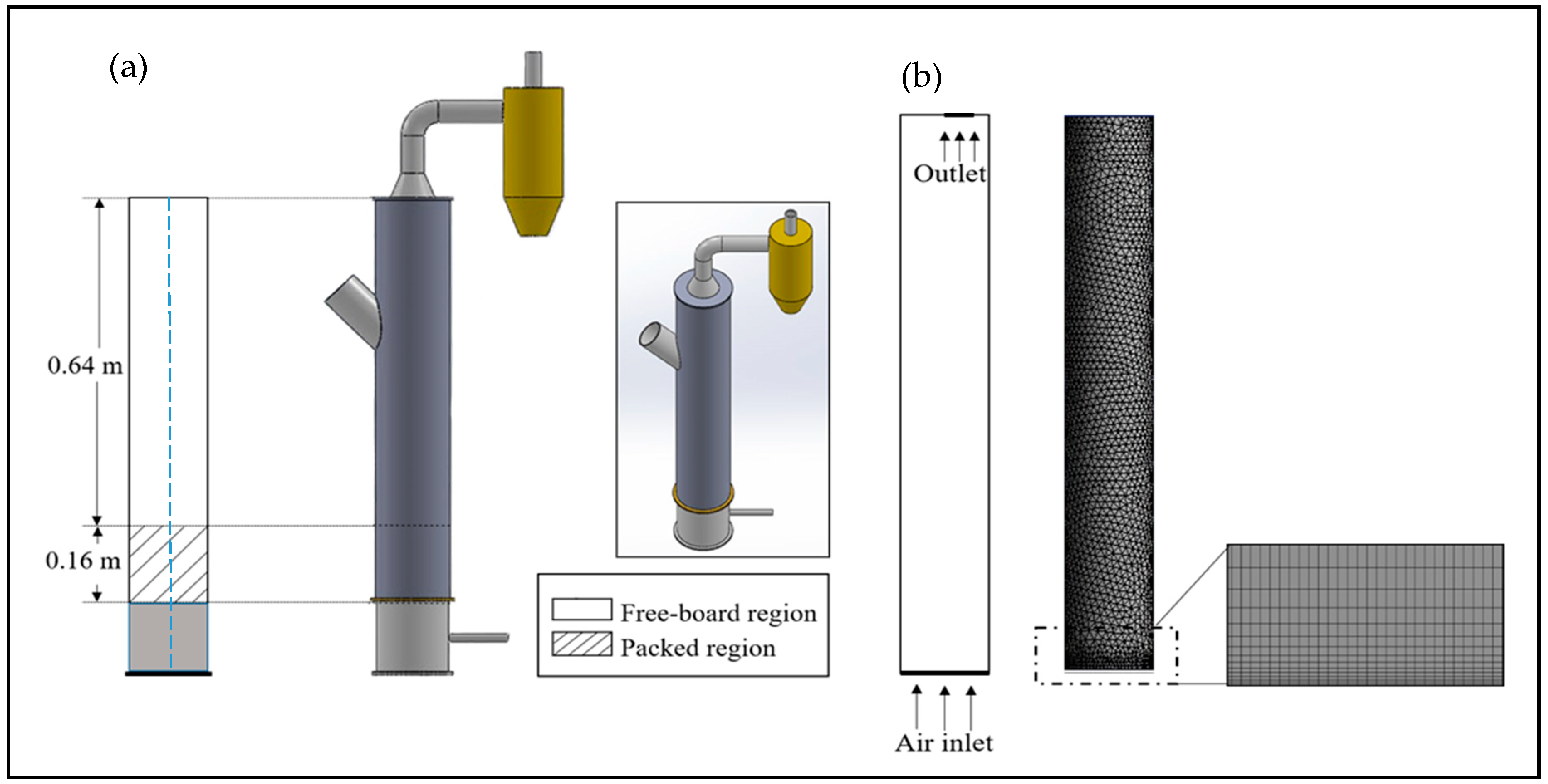
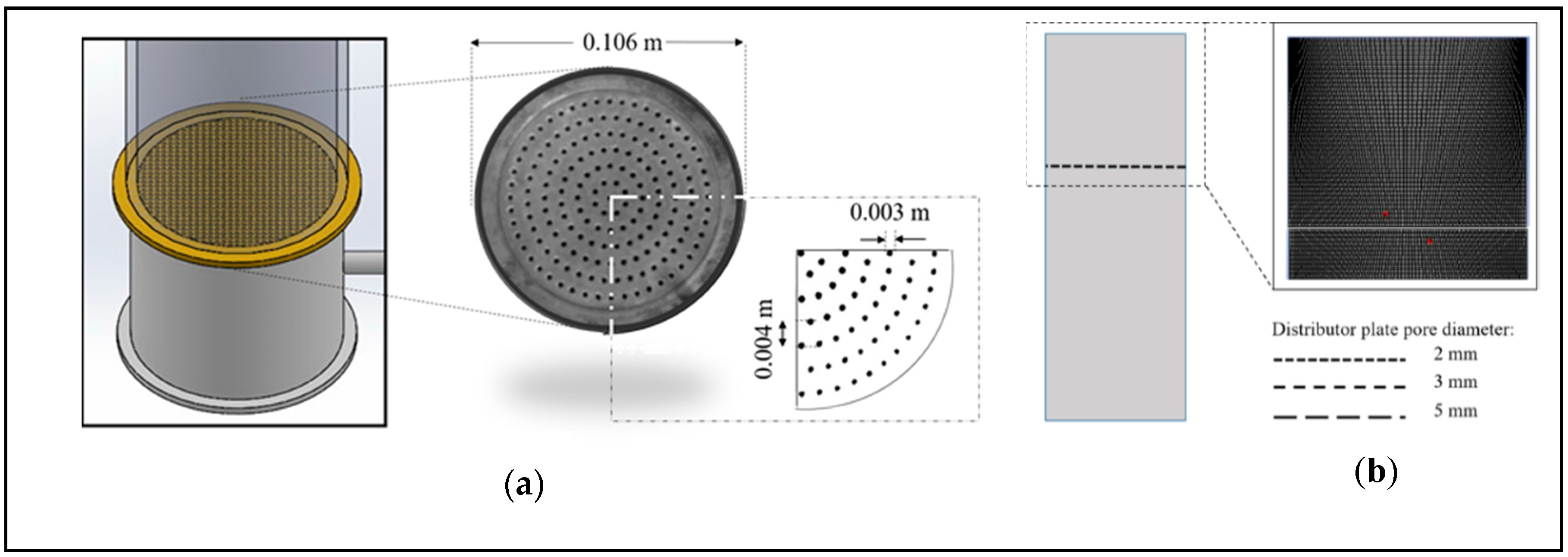
2.2.1. Initial Conditions, Boundary Conditions, Geometry and Grids

The geometry, boundary conditions and grids of the reactor at the initial state are defined and shown in Figure 1a,b, in order to study the fluidization of the granular biomass particles.
Air (i.e., the fluidizing agent) enters the reactor from the bottom and passes through a distributor plate prior to its injection into the chamber. The producer gas exits from the top of the reactor where the pressure is set to atmospheric with no backflow pressure. The walls are thermally insulated and defined with a specularity coefficient of ϕ = 0.5 for the solid phase, as recommended for multiphase granular flow on bubbling fluidized beds and a no-slip condition for air [32]. Up to 20% of the reactor volume was initially packed with bed material (i.e., silica sand). The volume fraction of solid particles within the patched zone was adjusted to 60%. The ambient air temperature and pressure were set at the reference values.
In order to avoid instability and poor convergence in the simulation of the multiphase flows, a small time step-size of 0.001 s with 100 iterations per time-step was used until the relative convergence criterion of 1 × 10⁻³ was satisfied. The physical specifications of the bed material are summarised in Table 2.
A fine grid was selected to capture the steep gradients between the neighbouring areas. The non-uniform grid spacing was generated using Ansys Desing Modeler (Figure 1). The second order upwind scheme was used to discretise the convective terms in the momentum and energy equations. The values and parameters used in the grid generation and numerical model development are shown in Table 3.

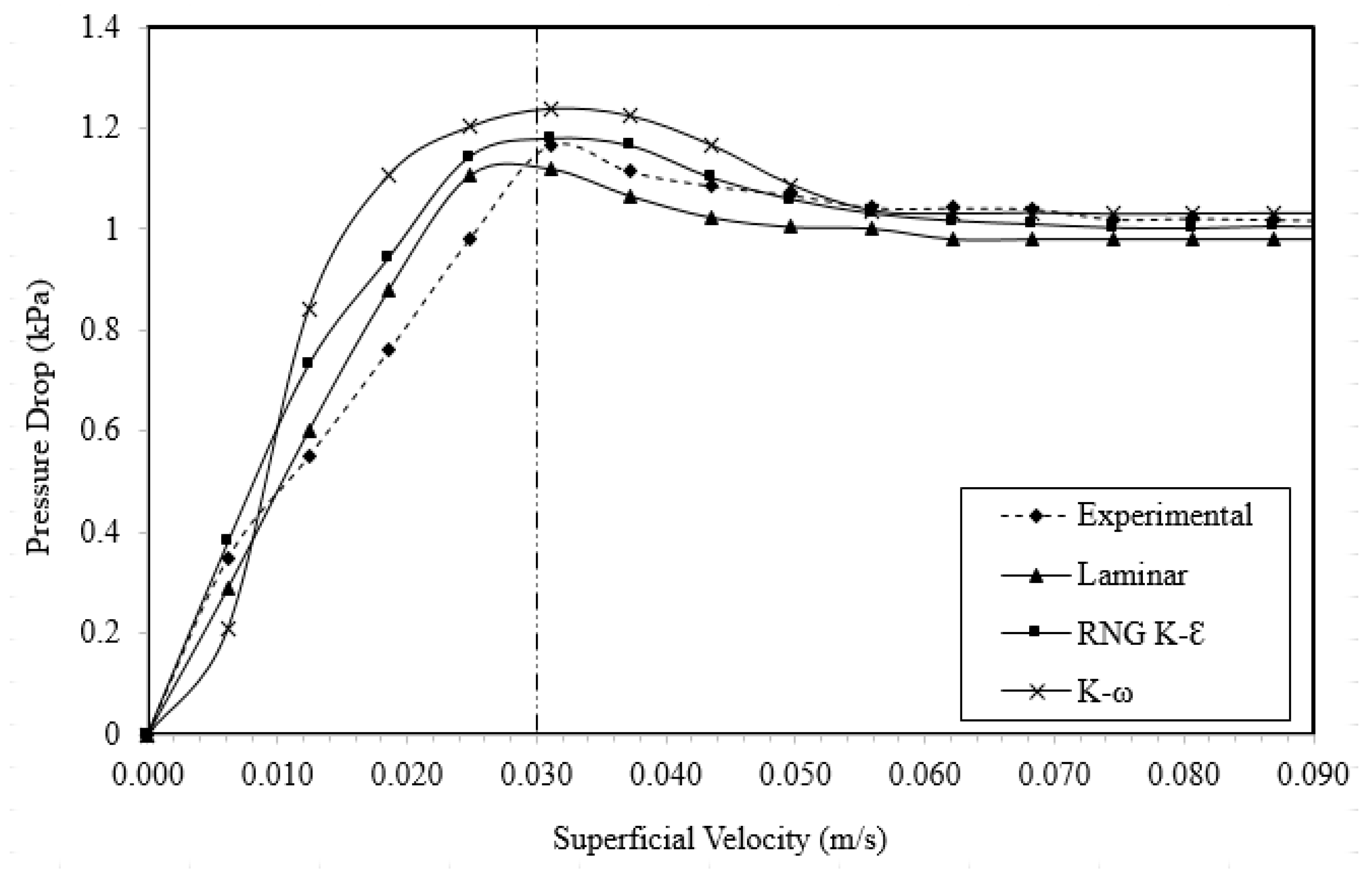
2.2.2. The Effect of Viscous Models on Pressure Drop Profile

The pressure drop profiles against different superficial velocities were derived for each viscous model (i.e., laminar, RNG k-ε and k-ω) and were then compared against the experimental data. It must be noted that the occurrence of pressure drop was due to continual fission and fusion of the bubbles in the fluidization zone [35]. The pressure drop values were recorded over the hypothetical vertical line aligned in the centre of the reactor’s geometry (Figure 1a).
The best viscous model was selected based on how accurately it could describe the pressure drop profile when compared with the experimentally-obtained data. That model was subsequently used for further analysis. In order to identify such a model, a statistical method was employed to evaluate a two-sample-T-test and to calculate the mean squared error (MSE) for each curve. In order to ensure that the bed has been effectively fluidized, the velocities <minimum fluidization velocity (Umf) were discarded in the statistical comparison.

2.2.3. Experimental Validation of the Numerical Analyses

Controlled experiments were conducted using a fluidized bed reactor in order to validate the simulation results. A reactor with similar dimensions and physical characteristics assumed in the modelling work, was used in experimental data collection. Pressure drop profiles were generated from the cold test evaluation when the reactor was initially packed with bed material with similar particle diameter (i.e., 550 µm) as assumed in the modelling, to the same level (i.e., 20% of total reactor volume) as described earlier in this work. Further details on the reactor specifications and experimental setup can be found in our previous study [36]. Each incremental drop in pressure throughout the reactor was caused by the gradual increase in the superficial velocity of the air between the air distributor and the reactor outlet.

2.2.4. The Effect of Air Distributor on Fluid Properties

The nature of the turbulence caused by the passage of the fluid through the air distributor was investigated. The area below and above the air distributor plate located at the bottom of the reactor was modelled. The dynamics of the air passing through the distributor plates (with pore diameters of 2, 3 and 5 mm) was selected for our simulation. The properties of the fluid with a superficial velocity of 0.2 ms−1 was described by the RNG K-Ɛ turbulent model in this section. The selected superficial velocity was about five times greater than the minimum fluidization velocity to ensure complete fluidization [9,37].
A mesh-structured air distributor plate was placed at the bottom of the reactor (Figure 2a). It was necessary to provide a regulated momentum of air inside the reactor chamber to avoid the falling back of the solid particles into the distributor zone, which could consequently have blocked the air nozzles. Distributor plates with different pore sizes (Figure 2b) were used in this simulation to investigate the effect of each perforated plate on the turbulent viscosity of the air. Although the diameter of the plate’s air holes was variable, the total area of the pores was intended to be constant by adjusting the number of the pores accordingly.

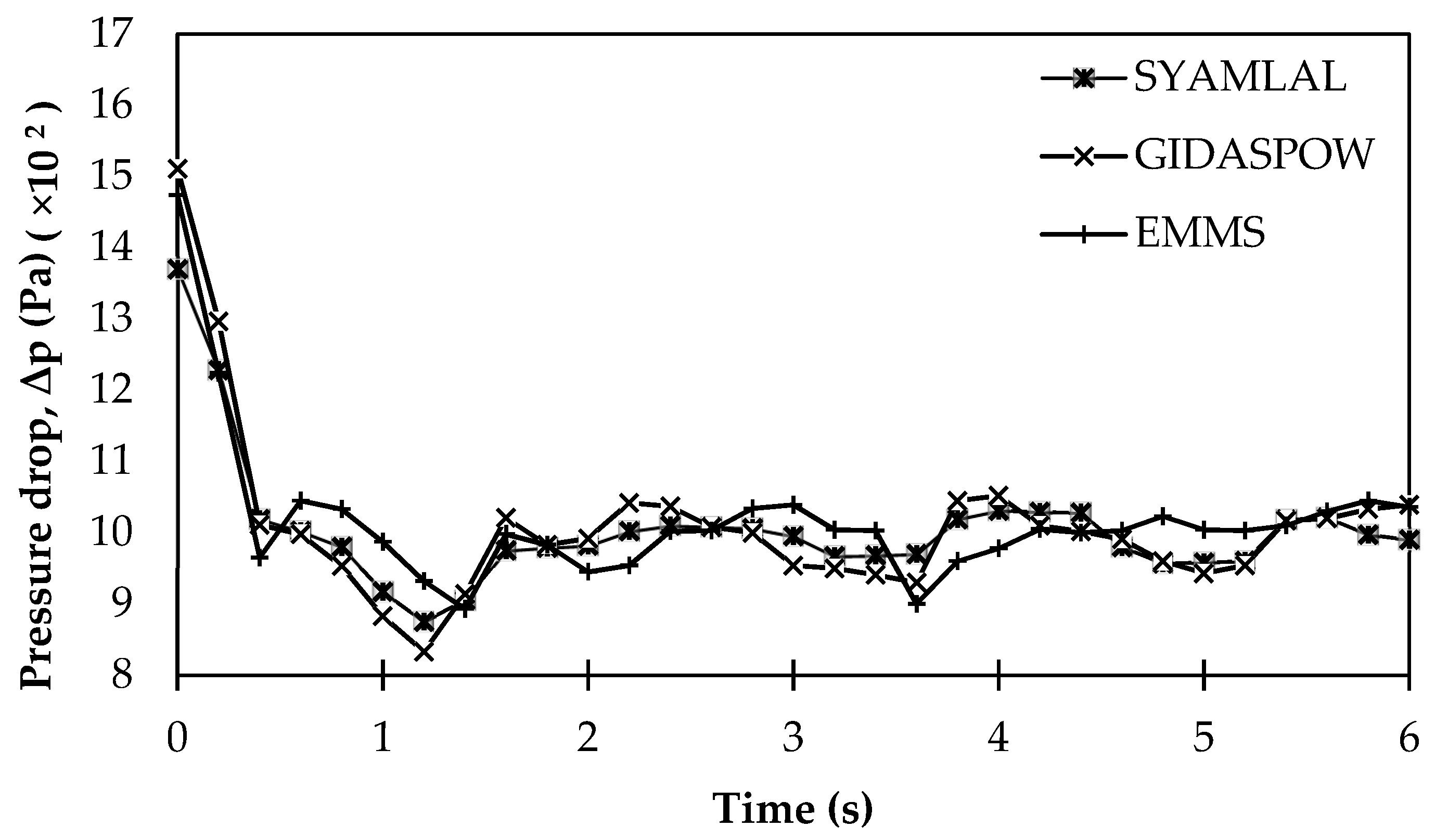
2.2.5. The Effect of Drag Models on Fluidization Hydrodynamics

Drag force is an key dominant force between the solid particles and the gas phase in a fluidized bed reactor [38]. Typically, the drag law describing the inter-phase momentum exchange is described by experimentally-developed models. However, for a fluidized bed with particular characteristics, it was necessary to investigate whether such models are still applicable. Therefore, three drag models (i.e., Syamlal–O’Brien, Gidaspow and EMMS) were selected in this study to numerically investigate the effect of drag functions on the fluidization hydrodynamics. Initially, the pressure drop throughout the bed was recorded over time for each drag model. That helped to understand when the impact of pressure drop began to diminish and a steady-state was reached. That indicates complete fluidization where the bed has been expanded to its maximum target capacity. At that point, the hydrodynamics of gas–solid fluidization can be defined on a time-averaged basis. Subsequently, the effect of drag models on the volume fraction of the particles was investigated.

2.2.6. Integrated Turbulent Model and Model Validation

A comprehensive model of the fluidization of the granular particles was be developed via the integration of the optimum parameters obtained for the most suitable viscosity, drag and pore size of the air distributor pore models for each stage. The contours of particles’ volume fraction obtained from the turbulent model were compared with the standard laminar model in a similar setup. It must be noted that the term “solid” in this study refers to the particle materials in the bed (i.e., granular silica sands). It is of key importance to achieve a well-developed fluidized bed in terms of bed expansion and pressure gradient prior to injecting the biomass into the reactor. Moreover, in the actual process, the biomass particles degrade immediately as injected into the hot reactor and undergo a drastic loss in density while converting into the solid biochar within a very short period of time. The density of the produced char is about 40 times less than the bed material (i.e., 2636 kg m−1) (e.g., Napier grass biochar has the density of 71 kg m−1 [36]). Therefore, it was not possible for the fluidizing agent to overcome the drag force, and as a consequence, the particles would fly out of the reactor. Therefore, the characteristics of fluidization, such as the minimum fluidization condition, maximum bed expansion and the bubble formation are mostly governed by the motion pattern of the sand particles and are less effected by the biomass particles.
Once the final integrated model has been set up, it is capable of monitoring the solid volume fraction profile inside the reactor throughout the gasification process. It enabled us to also predict the parameters associated with the particles’ motion and the physical aspects of the fluidization, including the kinetic parameters, pressure-related characteristics, formation and transportation of bubbles and the parameters associated with the fluidized bed expansion.

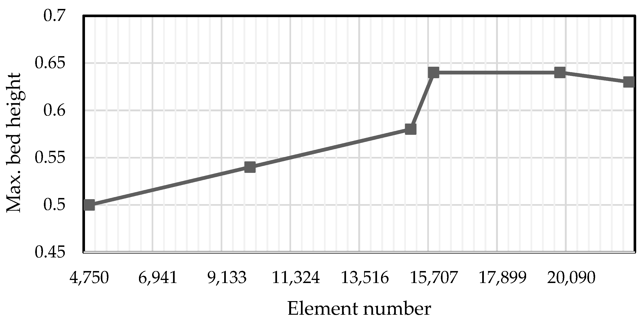
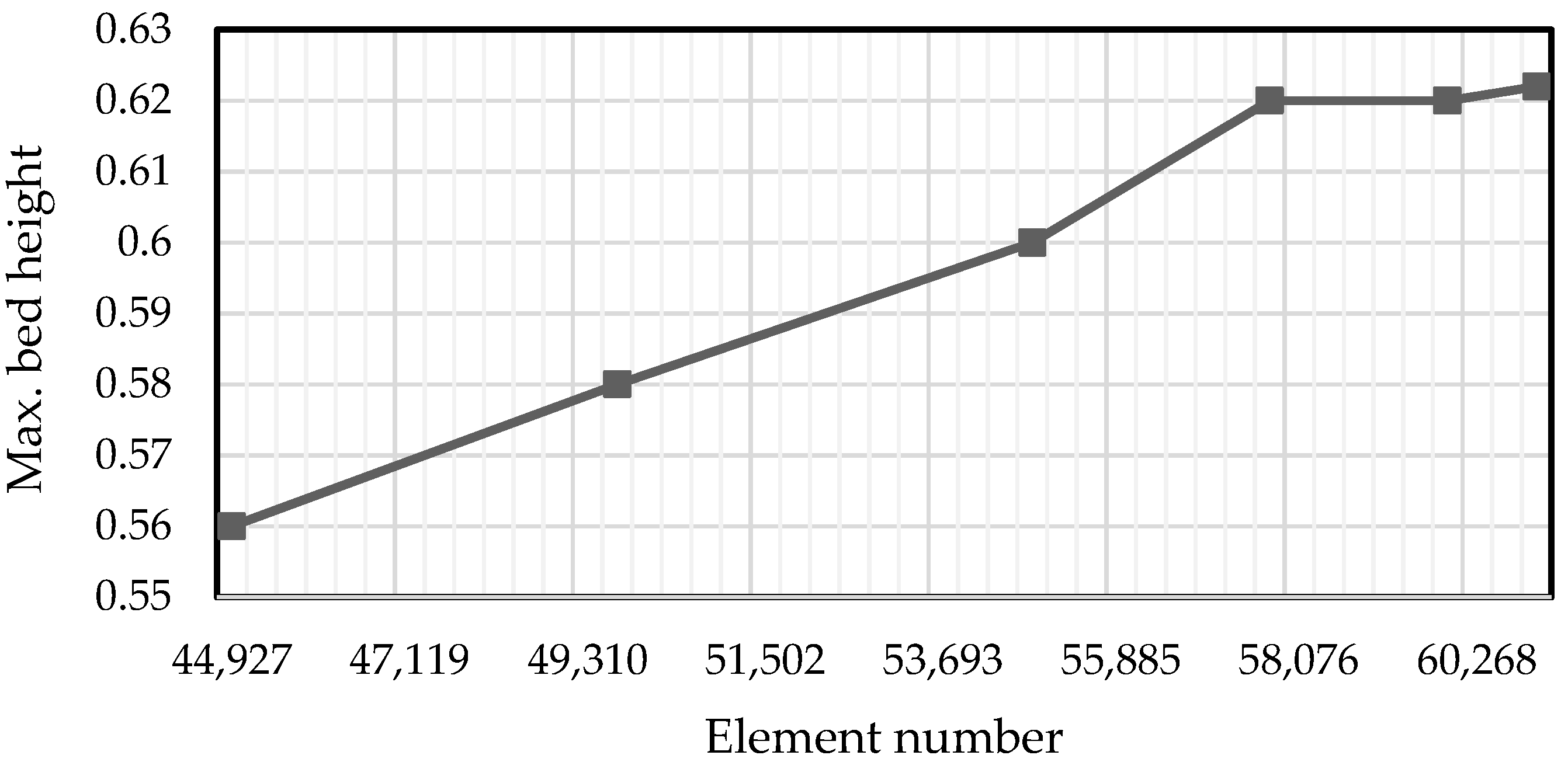
2.2.7. Grid Resolution Study

Grid resolution study was conducted in order to check the accuracy of the results. This was done by pursuing the balance between coarseness of the mesh elements and the computation time required for a solution. Indeed, coarser grids require less computation time and vice versa. The procedure starts with selecting a coarse grid with the least number of elements and performing the computation until the results have been converged with lower relative errors than the pre-defined limit (i.e., 5 × 10⁻⁴) for all models involved in this study. Similar grid sizes and numbers of elements were used in both studies of fluidization hydrodynamics and evaluation of temperature gradient. Therefore, a single grid study was valid for both models. The results of grid resolution tests are shown in Figure 3 and Figure 4, respectively.
The output factor selected in this grid study was the maximum bed height and is related to the particles’ superficial velocities along the y-axis. Maximum bed expansion occurs when a particle with the highest y value in all time steps has the velocity of zero. Zero y-velocity with highest possible elevation means that the particle is not travelling to any higher zones, and thus, merely bounces within the fluidization region. An accurate grid quality for a reasonable computation time ensures the highest bed expansion and better fluidization characteristics. For the laminar model, the computations were completed for six runs while each run was committed to a gradual increase in element numbers and eventually converged within a specific time window. Figure 3 shows that the bed height does not significantly increase with finer grid structure above 16,000 elements. Any further increase in element quantities above this point leads to an unnecessarily prolonged computing time. The same trend was observed in the turbulent model but with 58,000 elements (Figure 4). Those optimum grid qualities were employed in the evaluation of the models in this work.

3. Result and Discussion

3.1. The Effect of Viscous Models on Pressure Drop Profiles

The modelled pressure drop profiles against the superficial velocities corresponding to each viscous model are shown in Figure 5.
In the laminar regime, the uniform flow of the inlet air stream shows insignificant acceleration, and hence, appears to follow the Hagen–Poiseuille equation order [39]. According to Figure 5, although different pressure drop values are indicated by each model, the minimum fluidization velocities (Umf) are just slightly different. The values of Umf are 0.030, 0.029, 0.031 and 0.037 (ms−1) for experimental, laminar, RNG K-Ɛ and K-ω models, respectively.
At lower superficial velocities, an increase in the pressure drop in the laminar model is seen with a constant slope until the maximum Δp is reached. This can be due to the uniform and vibrating motion of the static bed as well as the regular pressure drop gradient [40]. For the velocities below Umf, an increase in the superficial velocity leads to an increase in the pressure drop; however, the slope was observed to be steeper for the RNG K-Ɛ and K-ω models compared to the laminar model. That can be explained by the different functions of each model in describing the particle interactions and parameters, such as friction coefficient, shear stress, formation of eddies and the associated transferred energy [41]. All models tend to converge and surpass at the onset of fluidization when the superficial velocity is over 0.03 ms−1. The Δp is then recorded at constant pressure of 1.016 kPa during the experimental trial: 0.980 kPa for laminar, 1.001 kPa for RNG K-Ɛ and 1.032 kPa for K-ω models.
According to the statistical analyses, only the two laminar and RNG K-Ɛ models with p-values of <0.05 were capable of adequately representing the experimental data. The RNG K-Ɛ with a smaller MSE of 539 was selected as the most desirable model for this study to further describe the turbulent characteristics of the fluidization hydrodynamics.

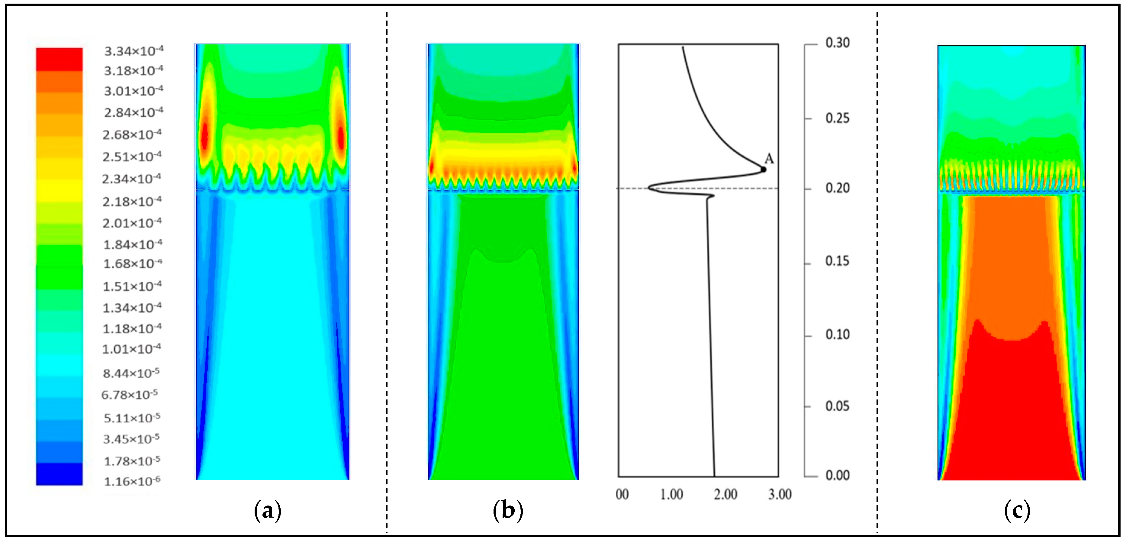
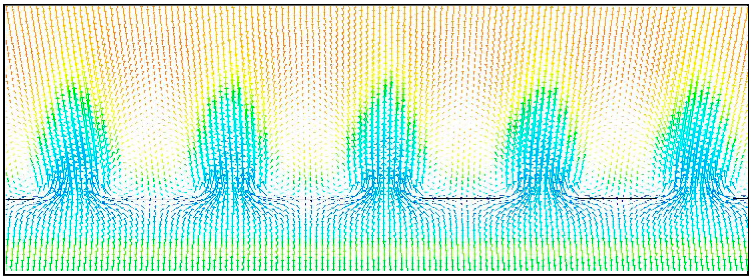
3.2. The Effect of Air Distributor on the Fluid Properties

In this study, the effect of air distributor on the fluid properties was investigated and an effective turbulent viscosity was calculated to analyse the transfer of momentum caused by turbulent eddies. The corresponding contours of the turbulent viscosity across the distributor area are presented in Figure 6.
The air distributor with larger pores (Figure 6a) was observed to be less effective in increasing the magnitude of the kinetic energy of the fluid. Moreover, the pressure gradient is not uniformly distributed above the surface of the plate. The energy that is introduced by eddies are maximized around the corners which may result in pushing the solid particles to travel along the wall zones and less towards the centre of the reactor. This may cause a sudden pressure drop across the centre which simultaneously reduces the bed expansion. Plates with pore diameters of <5 mm are, therefore, desirable. However, according to Figure 6c, very small pore diameters also tend to be non-ideal as they increase the turbulent viscosity, as well as the gas pressure below the distributor plate. Therefore, they create the red zone—an indication of the air failing to pass through the nozzles. This is due to the fact that the sudden pressure drop imposed by the very small pores leads to the overall pressure of the fluid below the plate to significantly increase [42]. Larger eddies are created across the plate and the chance of a back pressure developing increases. The velocity of the fluid above the distributor plate, on the other hand, is too small to vibrate the solid particles, hence is not able to expand the bed. A plate with a pore diameter of 3 mm (Figure 6b) was observed to have a better turbulent viscosity profile than the other two cases discussed. The distribution of energy above the plate is uniform and the viscosities are maximal (i.e., a 1.8 fold increase). Although the intensity of turbulent viscosity is higher around the wall area, it is relatively constant towards the centre of the plate.
A plot of the turbulent viscosity against the centre line of Y-coordinates is shown in Figure 6b. The turbulent viscosity of the air was slightly reduced from 1.79 × 10⁻⁴ to 1.65 × 10⁻⁴ kg(ms)−1 from the heights of 0 to 0.18 m. However, as the fluid touches the distributor plate, the turbulent viscosity, encountered by an intensive pulse, passes through the grate pores. At the beginning, it rapidly increases to 1.7 × 10⁻⁴ kg(ms)−1 at a height of 0.196 m and then dramatically drops to 0.58 × 10⁻⁴ kg(ms)−1 at a height of 0.2 m. It then increases to the maximum value of 2.69 × 10⁻⁴ kg(ms)−1 at point “A” at a height of 0.217 m and then falls again as it exits from the pores of the mesh structured plate, and flows along the height of reactor until it reaches 1.21 × 10⁻⁴ kg(ms)−1 at the height of 0.3 m. The resultant pulse was similar to the performance of an air nozzle, indicating a rapid rise in the kinetic energy by applying a sudden pressure drop to the fluid that is passing through the narrow channels of the nozzle [43]. For a better visualization of the phenomena, a closer view of the fluid momentum when passing through the nozzles is shown in Figure 7 with the assistance of velocity vectors.
A sudden pressure drop is observed when the upwards-moving fluid reaches the small air nozzles. The air molecules are contracted as a result and their kinetic energy reduces accordingly while passing through the nozzles. Molecules with a high potential energy eject from the pores to above the distributor plate as their energy converts to kinetic energy in a very short time span, creating the eddies with the highest motions [42]. Since the fluid velocity is adequate and the pore diameters are defined properly, the turbulent viscosity profile becomes consistent from across the top of the plate and creates a steady pressure profile for fluidization. An air distributor plate with a pore diameter of 3 mm was, therefore, considered desirable in this study and will be used for further hydrodynamics investigations. Also, all the calculated quantities corresponding to the turbulent fluidizing fluid have been employed to derive the properties at point “A” in Figure 6b.

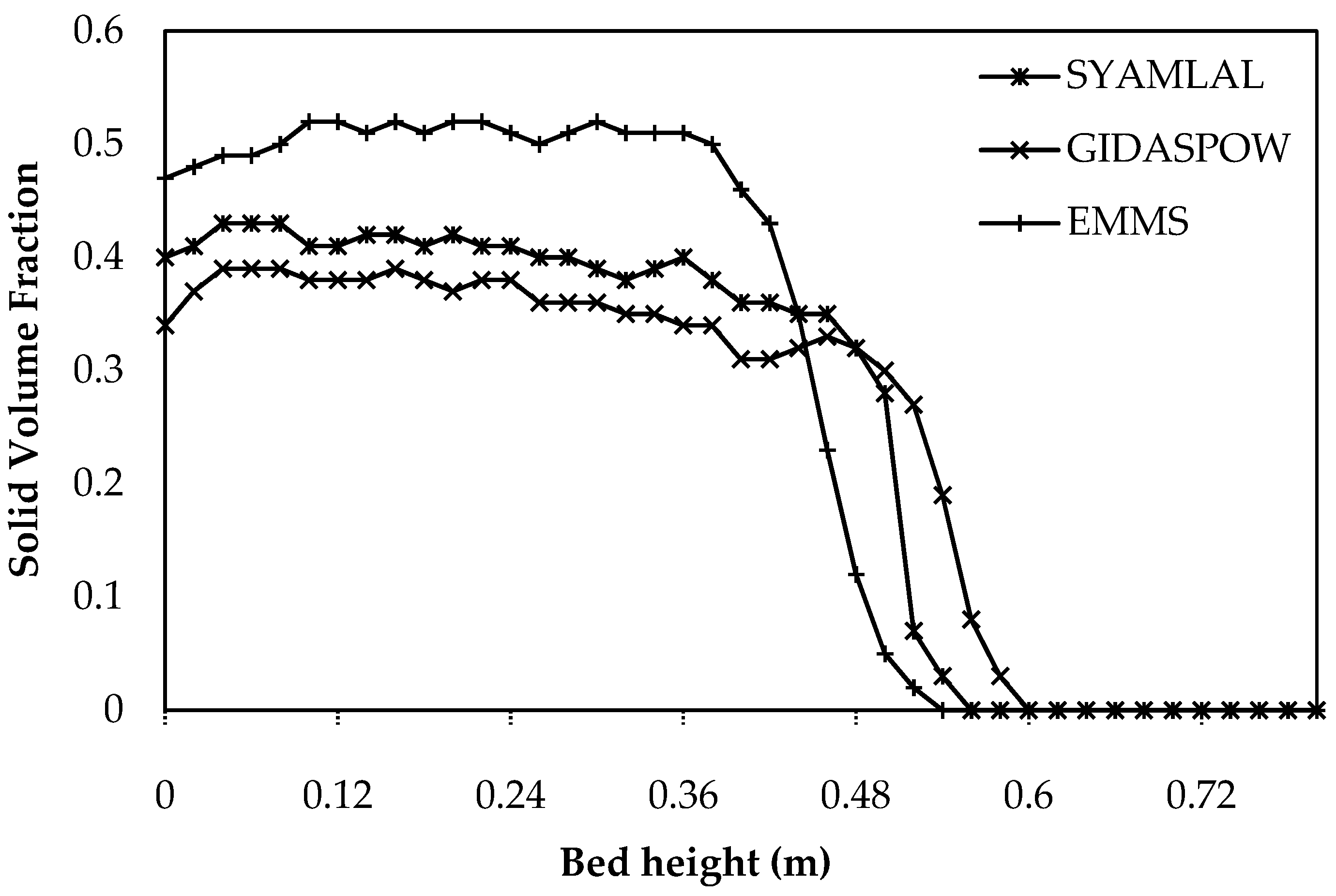
3.3. The Effect of Drag Models on Fluidisation Hydrodynamics

The results of pressure drop versus time for the three drag models used in this study are shown in Figure 8. It is observed that the pressure drop corresponding to all the three drag models have considerably reduced and hit a minimum at the beginning of the fluidization in approximately 1.5 s.
However, the pressure drop began to slightly increase until it reached a relatively steady-state condition with least fluctuation after almost 3 s.
Figure 9 indicates the variation of time-averaged solid volume fraction as the result of using the selected drag models along the height of the reactor at the central axis. It is seen that the models predicted by Syamlal–O’Brien and Gidaspow showed relatively lower solid volume fractions at any heights below 0.4 m as compared to the EMMS. However, the overall bed expansion for the model predicted by the EMMS was smaller (i.e., 0.54 m) than those forecast by Syamlal–O’Brien (i.e., 0.58) and Gidaspow (i.e., 0.6). Furthermore, the solid volume fraction at the surface of the fluidized bed gradually dropped to zero for the models predicted by Syamlal–O’Brien and Gidaspow, which seemed to be more physically realistic than those predicted by the EMMS.
The EMMS model unrealistically predicts too sharp of a change in the solid volume fraction at similar zones. According to the pressure drop values corresponding to the three drag models (Figure 8), the formation of bubbles and the motion of particles are expected to follow a similar trend; however, the effects of each on the bed expansion and solid volume fraction are significant. The pressure drop corresponding to the minimum fluidization condition obtained experimentally (i.e., 1.166 kPa) was compared to that from the simulation of the drag models. The value obtained from the Syamlal–O’Brien model (i.e., 1.123 kPa) is observed to be more consistent with the experimental data, and therefore, it was considered as the reference drag model in the development of the hydrodynamic model.

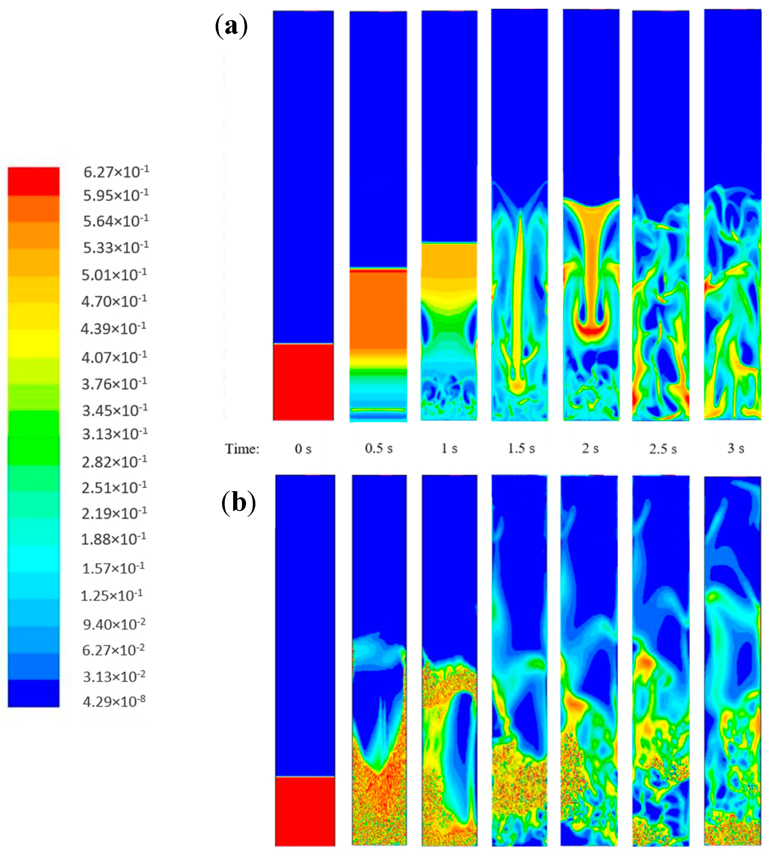
3.4. Development of the Fluidisation Hydrodynamics Turbulent Model

The hydrodynamics of fluidization was simulated with the RNG K-Ɛ turbulent model and the Syamlal–O’Brien drag model. An air distributor with a pore diameter of 3 mm was assumed to define the momentum exchange between the gas and solid phases, inter-particle interactions, bubble formation and motion pattern of the bed material in the state of fluidization. The initial air velocity and the turbulent viscosity were 0.2 ms−1 and 2.69 × 10⁻⁴ kg(ms)−1, respectively. The process was simulated for the initial 3 s. The contours for the solid volume fractions corresponding to different time steps-starting from the initial condition (i.e., t = 0) and continuing for three seconds of complete fluidization, are illustrated in Figure 10.
The formations of bubbles as well as the maximum bed expansion were noticeable at each time step. Both systems gradually reached a steady state and became fully-developed within three seconds once the fluidization was initiated. The particles in the laminar model (Figure 10a) are seen to have an axisymmetric distribution. The bubbles began to form at the surface of the air distributor and were enlarged as they moved upwards due to the surface tension gradient. Similar hydrodynamic behaviour has been reported previously [10,13]. However, as depicted in Figure 10b, the formation and development of bubbles as described by the RNG k-Ɛ turbulent model seems to be non-uniform when compared to that described by the laminar model. Large quantities of small bubbles are firstly formed at the surface of the air distributor as opposed to the laminar model. These bubbles then gradually distributed towards the bed medium—more likely closer to the wall. The enlargement of the bubbles close to the wall was due to the friction caused by the wall roughness. The momentum imparted to the walls was introduced by the specularity coefficient for the solid phase at wall conditions. However, the bubbles in the middle section of the chamber were developed in size and quantity due to the interaction with the smaller nearby bubbles. All bubbles formed eventually tend to migrate to and collapse at the bed surfaces. Similar behaviour of bubbling fluidized beds is described in a previous study [44] as the bubbles started to form and expand in diameters prior to upwards movement through the bed medium towards the free board region. The movements of the bubbles, as they collide with the stationary particles, transfers the kinetic energy and causes them to travel in random directions along the height of the gasifier and hence, establishing the fluidization phenomenon.

4. Conclusions

A numerical model with a Eulerian—Eulerian multiphase approach was employed to simulate biomass gasification in a bubbling fluidized bed reactor. Different turbulent models were investigated to study the hydrodynamics of the gasification process. The pressure drop was modelled along the gasifier’s height for various superficial velocities, and the results were compared and validated against the experimentally-obtained data. The values corresponding to the RNG k-Ɛ turbulent model were seen to have a better description of the experimental results. Moreover, the impact of the air distributor, with different pore diameters on the momentum characteristics of the air as it enters the gasifier, was investigated. The distributor plate with a pore diameter of 3 mm was selected for generating the largest turbulent viscosities above the distributor’s plate (i.e., 2.69 × 10⁻⁴ kg(ms)−1) with a uniform distribution profile. The drag models of Syamlal–O’brien, Gidaspow and EMMS were investigated in solid fluidization in terms of pressure drop profiles and the volume fraction. In comparison, the Syamlal–O’Brien model corresponding to a pressure drop of 1123 Pa was observed to be the most consistent with the experimental data (i.e., 1166 Pa). Upon the integration of the models’ outputs, the contours for the solid volume fractions were generated and compared with the laminar model. The formation of the bubbles and their movement along the gasifier’s height as well as the pressure drop profiles in the presence of the turbulent flow followed a different pattern compared to the laminar flow. The developed hydrodynamic model was able to predict the numerical terms associated with the particles’ motions and the physical aspects of fluidization, including the kinetics, pressure-related characteristics, formation, and transportation of bubbles and fluidized bed expansion. The derived hydrodynamic model can also help to reduce the number of empirical trials required for process optimization for a fluidized bed reactor—providing accurate details on the physical aspects of fluidization which are challenging to experimentally measure.

Author Contributions

Conceptualization, R.K. and W.A.W.A.K.G.; Funding Acquisition, W.A.W.A.K.G.; Methodology, R.K.; Supervision, W.A.W.A.K.G., D.R.A.B., and R.Y.; Writing—Original Draft, R.K.; Writing—Review & Editing, W.A.W.A.K.G., S.M.S., M.S., S.R.M., and K.S.

Funding

This work has been funded and supported under the Ministry of Higher Education (MOHE) Malaysia via LRGS grant (Grant No. LRGS/2013/UKM/PT). Also, this research has been partially funded by the Engineering and Physical Sciences Research Council through the BEFEW project (Grant No. EP/P018165/1).

Acknowledgments

The authors would like to acknowledge the Chemical and Environmental Engineering Departments at University Putra Malaysia to support conducting this research.

Conflicts of Interest

The authors declare no conflict of interest.

References

  1. Khezri, R.; Azlinaa, W.; Tana, H.B. An Experimental Investigation of Syngas Composition from Small-Scale Biomass Gasification. Int. J. Biomass Renew. 2016, 5, 6–13. [Google Scholar]
  2. Ruiz, J.A.; Juárez, M.C.; Morales, M.P.; Muñoz, P.; Mendívil, M.A. Biomass gasification for electricity generation: Review of current technology barriers. Renew. Sustain. Energy Rev. 2013, 18, 174–183. [Google Scholar] [CrossRef]
  3. Santos, J.; Ouadi, M.; Jahangiri, H.; Hornung, A. Integrated intermediate catalytic pyrolysis of wheat husk. Food Bioprod. Process. 2019, 114, 23–30. [Google Scholar] [CrossRef]
  4. Maiti, S.; Sarma, S.J.; Brar, S.K.; Le Bihan, Y.; Drogui, P.; Buelna, G.; Verma, M. Agro-industrial wastes as feedstock for sustainable bio-production of butanol by Clostridium beijerinckii. Food Bioprod. Process. 2016, 98, 217–226. [Google Scholar] [CrossRef]
  5. Sansaniwal, S.K.; Rosen, M.A.; Tyagi, S.K. Global challenges in the sustainable development of biomass gasification: An overview. Renew. Sustain. Energy Rev. 2017, 80, 23–43. [Google Scholar] [CrossRef]
  6. Puig-Arnavat, M.; Bruno, J.C.; Coronas, A. Review and analysis of biomass gasification models. Renew. Sustain. Energy Rev. 2010, 14, 2841–2851. [Google Scholar] [CrossRef]
  7. Couto, N.; Silva, V.; Monteiro, E.; Brito, P.S.D.; Rouboa, A. Experimental and Numerical Analysis of Coffee Husks Biomass Gasification in a Fluidized Bed Reactor. Energy Procedia 2013, 36, 591–595. [Google Scholar] [CrossRef] [Green Version]
  8. Armstrong, L.M.; Gu, S.; Luo, K.H. Effects of limestone calcination on the gasification processes in a BFB coal gasifier. Chem. Eng. J. 2011, 168, 848–860. [Google Scholar] [CrossRef] [Green Version]
  9. Sau, D.C.; Biswal, K.C. Computational fluid dynamics and experimental study of the hydrodynamics of a gas–solid tapered fluidized bed. Appl. Math. Model. 2011, 35, 2265–2278. [Google Scholar] [CrossRef]
  10. Liu, H.; Yoon, S.; Li, M. Three-dimensional computational fluid dynamics (CFD) study of the gas–particle circulation pattern within a fluidized bed granulator: By full factorial design of fluidization velocity and particle size. Dry. Technol. 2017, 35, 1043–1058. [Google Scholar] [CrossRef]
  11. Hosseini, S.H.; Zivdar, M.; Rahimi, R. CFD simulation of gas–solid flow in a spouted bed with a non-porous draft tube. Chem. Eng. Process. Process Intensif. 2009, 48, 1539–1548. [Google Scholar] [CrossRef]
  12. Silaen, A.; Wang, T. Effect of turbulence and devolatilization models on coal gasification simulation in an entrained-flow gasifier. Int. J. Heat Mass Transf. 2010, 53, 2074–2091. [Google Scholar] [CrossRef]
  13. Xie, J.; Zhong, W.; Jin, B.; Shao, Y.; Liu, H. Simulation on gasification of forestry residues in fluidized beds by Eulerian–Lagrangian approach. Bioresour. Technol. 2012, 121, 36–46. [Google Scholar] [CrossRef] [PubMed]
  14. Abani, N.; Ghoniem, A.F. Large eddy simulations of coal gasification in an entrained flow gasifier. Fuel 2013, 104, 664–680. [Google Scholar] [CrossRef]
  15. Taghipour, F.; Ellis, N.; Wong, C. Experimental and computational study of gas-solid fluidized bed hydrodynamics. Chem. Eng. Sci. 2005, 60, 6857–6867. [Google Scholar] [CrossRef]
  16. Papadikis, K.; Gu, S.; Bridgwater, A.V. CFD modelling of the fast pyrolysis of biomass in fluidised bed reactors. Part B: Heat, momentum and mass transport in bubbling fluidised beds. Chem. Eng. Sci. 2009, 64, 1036–1045. [Google Scholar] [CrossRef]
  17. Armellini, V.A.D.; Di Costanzob, M.; Castroa, H.C.A.; Vergel, J.L.G.; Mori, M.; Martignonic, W.P. Effect of different gas-solid drag models in a high-flux circulating fluidized bed riser. Chem. Eng. 2015, 43, 1627–1632. [Google Scholar]
  18. Dhrioua, M.; Hassen, W.; Kolsi, L.; Anbumalar, V.; Alsagri, A.S.; Borjini, M.N. Gas distributor and bed material effects in a cold flow model of a novel multi-stage biomass gasifier. Biomass Bioenergy 2019, 126, 14–25. [Google Scholar] [CrossRef]
  19. Mehrabadi, M. Fluid-Phase Velocity Fluctuations in Gas-Solid Flows; Iowa State University Digital Repository: Ames, IA, USA, 2012. [Google Scholar]
  20. Liu, H.; Cattolica, R.J.; Seiser, R.; Liao, C. Three-dimensional full-loop simulation of a dual fluidized-bed biomass gasifier. Appl. Energy 2015, 160, 489–501. [Google Scholar] [CrossRef] [Green Version]
  21. Liu, H.; Elkamel, A.; Lohi, A.; Biglari, M. Computational Fluid Dynamics Modeling of Biomass Gasification in Circulating Fluidized-Bed Reactor Using the Eulerian–Eulerian Approach. Ind. Eng. Chem. Res. 2013, 52, 18162–18174. [Google Scholar] [CrossRef]
  22. Cai, J.; Wang, Y.; Zhou, L.; Huang, Q. Thermogravimetric analysis and kinetics of coal/plastic blends during co-pyrolysis in nitrogen atmosphere. Fuel Process. Technol. 2008, 89, 21–27. [Google Scholar] [CrossRef]
  23. Huang, J.; Lu, Y.; Wang, H. Fluidization of Particles in Supercritical Water: A Comprehensive Study on Bubble Hydrodynamics. Ind. Eng. Chem. Res. 2019, 58, 2036–2051. [Google Scholar] [CrossRef]
  24. Yancheshme, A.A.; Zarkesh, J.; Rashtchian, D.; Anvari, A. CFD Simulation of Hydrodynamic of a Bubble Column Reactor Operating in Churn-Turbulent Regime and Effect of Gas Inlet Distribution on System Characteristics. Int. J. Chem. React. Eng. 2016, 14, 213–224. [Google Scholar] [CrossRef]
  25. Yu, G.; Ni, J.; Liang, Q.; Guo, Q.; Zhou, Z. Modeling of Multiphase Flow and Heat Transfer in Radiant Syngas Cooler of an Entrained-Flow Coal Gasification. Ind. Eng. Chem. Res. 2009, 48, 10094–10103. [Google Scholar] [CrossRef]
  26. Wang, S.; Luo, K.; Hu, C.; Fan, J. CFD-DEM study of the effect of cyclone arrangements on the gas-solid flow dynamics in the full-loop circulating fluidized bed. Chem. Eng. Sci. 2017, 172, 199–215. [Google Scholar] [CrossRef]
  27. Wu, Y.; Liu, D.; Ma, J.; Chen, X. Effects of gas-solid drag model on Eulerian-Eulerian CFD simulation of coal combustion in a circulating fluidized bed. Powder Technol. 2018, 324, 48–61. [Google Scholar] [CrossRef]
  28. Wang, J.; Ge, W.; Li, J. Eulerian simulation of heterogeneous gas–solid flows in CFB risers: EMMS-based sub-grid scale model with a revised cluster description. Chem. Eng. Sci. 2008, 63, 1553–1571. [Google Scholar] [CrossRef]
  29. Ku, X.; Li, T.; Løvås, T. Eulerian–Lagrangian Simulation of Biomass Gasification Behavior in a High-Temperature Entrained-Flow Reactor. Energy Fuels 2014, 28, 5184–5196. [Google Scholar] [CrossRef]
  30. Wilcox, D. A half century historical review of the k-omega model. In Proceedings of the 29th Aerospace Sciences Meeting, Reno, NV, USA, 7–10 January 1991; p. 615. [Google Scholar]
  31. Perini, F.; Zha, K.; Busch, S.; Reitz, R. Comparison of Linear, Non-Linear and Generalized RNG-Based K-Epsilon Models for Turbulent Diesel Engine Flows; SAE: Warrendale, PA, USA, 2017. [Google Scholar]
  32. Lan, X.; Xu, C.; Gao, J.; Al-Dahhan, M. Influence of solid-phase wall boundary condition on CFD simulation of spouted beds. Chem. Eng. Sci. 2012, 69, 419–430. [Google Scholar] [CrossRef]
  33. Khezri, R.; Azlina, W.; Ab, W.; Ghani, K. Computational Modelling of Gas-Solid Hydrodynamics and Thermal Conduction in Gasification of Biomass in Fluidized-Bed Reactor. Chem. Eng. Trans. 2017, 56, 1879–1884. [Google Scholar]
  34. Burns, A.D.; Frank, T.; Hamill, I.; Shi, J.-M. The Favre averaged drag model for turbulent dispersion in Eulerian multi-phase flows. In Proceedings of the 5th International Conference on Multiphase Flow (ICMF), Yokohama, Japan, 30 May–4 June 2004; Volume 4, pp. 1–17. [Google Scholar]
  35. Jiang, F.; Zhao, P.; Qi, G.; Li, N.; Bian, Y.; Li, H.; Jiang, T.; Li, X.; Yu, C. Pressure drop in horizontal multi-tube liquid–solid circulating fluidized bed. Powder Technol. 2018, 333, 60–70. [Google Scholar] [CrossRef]
  36. Khezri, R.; Wan Ab Karim Ghani, W.A.; Awang Biak, D.R.; Yunus, R.; Silas, K. Experimental Evaluation of Napier Grass Gasification in an Autothermal Bubbling Fluidized Bed Reactor. Energies 2019, 12, 1517. [Google Scholar] [CrossRef]
  37. Pérez, N.P.; Pedroso, D.T.; Machin, E.B.; Antunes, J.S.; Verdú Ramos, R.A.; Silveira, J.L. Fluid dynamic study of mixtures of sugarcane bagasse and sand particles: Minimum fluidization velocity. Biomass Bioenergy 2017, 107, 135–149. [Google Scholar] [CrossRef] [Green Version]
  38. Hua, L.; Zhao, H.; Li, J.; Wang, J.; Zhu, Q. Eulerian–Eulerian simulation of irregular particles in dense gas–solid fluidized beds. Powder Technol. 2015, 284, 299–311. [Google Scholar] [CrossRef]
  39. Gooch, J.W. Hagen-Poiseuille equation. In Encyclopedic Dictionary of Polymers; Springer: Berlin/Heidelberg, Germany, 2011; p. 355. [Google Scholar]
  40. Ismail, T.M.; Abd El-Salam, M.; Monteiro, E.; Rouboa, A. Eulerian—Eulerian CFD model on fluidized bed gasifier using coffee husks as fuel. Appl. Therm. Eng. 2016, 106, 1391–1402. [Google Scholar] [CrossRef]
  41. Bakshi, A.; Altantzis, C.; Bates, R.B.; Ghoniem, A.F. Study of the effect of reactor scale on fluidization hydrodynamics using fine-grid CFD simulations based on the two-fluid model. Powder Technol. 2016, 299, 185–198. [Google Scholar] [CrossRef] [Green Version]
  42. Fu, W.; Li, Y.; Liu, Z.; Wu, H.; Wu, T. Numerical study for the influences of primary nozzle on steam ejector performance. Appl. Therm. Eng. 2016, 106, 1148–1156. [Google Scholar] [CrossRef]
  43. Bear, J. Dynamics of Fluids in Porous Media; Courier Corporation: Chemsford, MA, USA, 2013; ISBN 0486131807. [Google Scholar]
  44. Seo, M.W.; Nguyen, T.D.B.; Lim, Y., II; Kim, S.D.; Park, S.; Song, B.H.; Kim, Y.J. Solid circulation and loop-seal characteristics of a dual circulating fluidized bed: Experiments and CFD simulation. Chem. Eng. J. 2011, 168, 803–811. [Google Scholar] [CrossRef]
Figure 1. (a) Reactor geometry, (b) boundary zones and grid design at initial state (static bed).
Processes 07 00524 g001
Figure 2. Geometry, boundary condition and grid design for the air distributor plate used in (a) experimentation and (b) numerical studies.
Processes 07 00524 g002
Figure 3. Grid resolution test for laminar flow.
Processes 07 00524 g003
Figure 4. Grid resolution test for re-normalisation group (RNG) K-Ɛ turbulent flow.
Processes 07 00524 g004
Figure 5. Pressure drop versus superficial velocity for different fluid regimes.
Processes 07 00524 g005
Figure 6. Effect of distributor plate with pore diameters of (a) 5 mm, (b) 3 mm and (c) 2 mm on the turbulent viscosity of the fluid.
Processes 07 00524 g006
Figure 7. Vector velocity coloured by turbulent viscosity on the pores of the distributor plate.
Processes 07 00524 g007
Figure 8. Comparison of simulated bed pressure drop using Syamlal–O’Brien, Gidaspow and energy minimum multi-scale (EMMS) drag models (U = 0.2 ms−1; i.e., ∼5 Umf).
Processes 07 00524 g008
Figure 9. Effect of drag models on the variation of time-averaged solid volume fraction along the reactor height at the central axis.
Processes 07 00524 g009
Figure 10. Solid volume fraction contours in a (a) laminar model and a (b) RNG k-Ɛ turbulent model.
Processes 07 00524 g010
Table 1. Governing equations of momentum and continuity for gas–solid phases [20,21,22,23,24,25].
Gas Phase Conservation Equations
Continuity equation t ( δ g ρ g ) + y ( δ g ρ g u ¯ ) = 0
Momentum equation t ( ρ V ) + . ( ρ V V ) =   P + . ( τ ¯ ¯ ) + ρ g + F
Solid Phase Conservation Equations
Continuity equation t ( δ s ρ s ) + y ( δ s ρ s u ¯ ) = 0
Momentum equation t ( ρ s δ s v ) + y ( ρ s δ s vv ) =   P s y ( δ s s ) y + δ s ρ s g + β g ( u ¯ v )
Table 2. Physical specifications of bed materials (silica sand particle) [33].
Physical PropertiesUnitQuantity
Density (Dry basis)(kg m−3)2636
Particle diameter(µm)550
Molecular weight(kg kmol−1)60
Table 3. Parameters used in grid generation and model development of fluidization hydrodynamics.
Model Statistics
Model basistransient
No. of elements58,000
Grid structureUnstructured
Turbulent multiphase modelDispersed
Turbulent dispersion modelAdopted from Burns et al. [34]

