Mathematical Modelling Forecast on the Idling Transient Characteristic of Reactor Coolant Pump

Abstract

The idling behavior of the reactor coolant pump is referred to as an important indicator of the safe operation of the nuclear power system, while the idling transition process under the power failure accident condition is developed as a transient flow process. In this process, the parameters such as the flow rate, speed, and head of the reactor coolant pump are all nonlinear changes. In order to ensure the optimal idling behavior of the reactor coolant pump under the power cutoff accident condition, this manuscript takes the guide vanes of the AP1000 reactor coolant pump as the subject of this study. In this paper, the mathematical model of idling speed and flow characteristic curve of reactor coolant pump under the power failure condition were proposed, while the hydraulic modeling database of different vane structure parameters was modeled based on the orthogonal optimization schemes. Furthermore, based on the mathematical modeling framework of multiple linear regressions, the mathematical relationship of the hydraulic performance of each guide vane in different parameters was predicted. The derived model was verified with the idling test data.

1. Introduction

In the case of a power outage, the reactor coolant pump will be forced to suspend its current operation due to the loss of power. Resulting from a consequent sudden reduction of coolant flow through the core of the reactor, the potential threat for the safety of the reactor is introduced. To ensure the nuclear safety of the reactor nuclear reaction boiling state [1], it is usually required that the core of the primary cooling loop shall be kept running by the unit for a certain period driven by rotational inertia. Therefore, the reactor coolant pump can generate enough flow to absorb the heat generated by the reactor in a short time after the power interruption. The capability of the reactor coolant pump to maintain operation by rotor inertia is called idling characteristics.

The reactor coolant pump coasting under power outage is commonly considered as a transient process. During the transition process of the reactor coolant pump stoppage, all the hydraulic parameters are forced to be continuously varied against times. The traditional velocity distribution, pressure distribution or streamlined diagram can be only applied to identify the overall quality of the flow field or to analyze the flow performance inside the impeller from a macro level. Many studies conducted by domestic and foreign scholars [1,2,3,4] can be referred to on the transient changes law after the power failure or shut-down of the reactor coolant pump. Zhang Senru [5] proposed a flow calculation model for the transient process of each loop of the nuclear power plant by using the coolant momentum conservation equation and the torque balance relation of the reactor coolant pump. Moreover, it was also found that the calculation model of the system flow characteristic curve was proposed by scholars like Guo Yujun [6] with the four-quadrant characteristic curve according to the torque balance relation of the reactor coolant pump. The computational model has proven to be important for analyzing the taxiing behavior of reactor coolant pumps. However, the coasting transient condition of the reactor coolant pump of Qinshan Nuclear Power Plant Phase II was calculated by Deng Shaowen [7] through the international conventional transient calculation method. The calculated flow curve of the reactor coolant pump was further compared with that given by the Framatome Atomic Energy Company, and the calculation results were consistent with the actual condition. However, it has also been found that scholars, such as Xu Yiming [8], simplify the calculation of the idling speed model of the reactor coolant pump after power failure through the torque balance relationship. Zhu Rongsheng studied the pressure pulsation characteristics of the reactor coolant pump at low flow conditions, and found that unstable pressure pulsation in the small flow condition was caused by the backflow in the impeller vane flow runner, the backflow mainly existed in the impeller and guide blade import and export [9]. Long Yun [10] and Feng Xiaodong [11] studied the vibration characteristics of the bearing seat in the coasting transition process of the reactor coolant pump in the power failure accidents and the internal flow characteristics of the pump under the condition of small flow. Alatrash, Y. [12] conducted an experimental study of the inertial pumping capability during the coastdown period to confirm whether the coastdown half time requirement given by safety analyses is being satisfied. In the modular modeling system(MMS) simulation model, all of the design data that affect the pump coastdown behavior are reflected. The experimental dataset is well predicted by the MMS model and is confirmed to be valid and consistent. For the study of reactor coolant pump, Brady, D. R. [13] proposed a method of upgrading a 1500 rpm reactor coolant pump motor having a vertically oriented rotor shaft supported by a lower guide bearing disposed of in an oil reservoir. Bang, S. Y. [14] mainly focuses on the performance requirements of the APR1400 and implements the safety, reliability and adaptability goals of the APR1400 system design, and describes the details of the development process, improved design features, and type test results. Metzroth, K. [15] used dynamic probabilistic risk assessment (PRA) methods combined with the MELCOR system code to check the behavior of RCP sealed loss of coolant accident (LOCA) and its impact on the evolution of SBO accident. It was found that the dynamic event tree (DET) analysis produced results were less conservative than those obtained in NUREG-1150, which had predicted larger leak rates earlier in the accident. Lu Y. et al. [16,17,18] studied the third and fourth generation reactor coolant pumps, main including gas-liquid two-phase flow and the transient characteristics of pump under extreme operating conditions, and finding in different gas fraction conditions, the homogeneous distribution of gas phase component in the fluid area was mainly related to the operating condition of pump, and when the volume flow rate deviates from the designed operating point, the fluid medium’s gas phase and liquid phase will separate to some extent.

On the premise of previous researches, the idling speed model of the reactor coolant pump to a reasonable extent by the momentum conservation equation was simplified by this paper, and the calculation model of coasting condition was further derived. Secondly, the hydraulic modeling database of different vane structure parameters was modeled under the orthogonal optimization schemes, and the mathematical relationship of the hydraulic performance of each guide vane in different parameter was predicted on mathematical modeling framework of multiple linear regression, by which the idling mathematical model of main geometrical parameters was derived. At last, the model was verified by the existing power outage test data, and the design criteria of the reactor coolant pump were further obtained from the modeling. Finally, the design parameters of the reactor coolant pump were calculated and verified.

2. Materials and Methods

2.1. Basic Theory of the Idling Condition of the Reactor Coolant Pump

The hydraulic performance and its idling characteristics of the reactor coolant pump are affected by different geometric parameters of guide vanes to a certain extent. The influence of different parameters of guide vane on the performance is not only determined by the size of a single geometric parameter, but also indirectly influenced by the mutual combination of the parameters due to their coupling relationship. Referring to the current research, the study of the idling characteristics of the reactor coolant pump is mainly focused on the idle half-flow time, in which the moment of inertia of the rotor component is much larger than the moment of inertia of the coolant inertia in the loop. Such influence can be ignored in idling mathematical modeling. Therefore, the water moment M_h and the friction torque M_f are both proportional to the square of the angular velocity ω. According to the torque balance principle of reactor coolant pump, a balance equation can be established as follows:

$$-I\frac{d\omega }{dt}=M_h+M_f=C{\omega }^2.$$

(1)

Refereed by the initial conditions t = 0, ω = ω₀, the solution of Formula (1) shall be:

$$\begin{array}{l}\omega =\frac{{\omega }_0}{1+t/t_p}\\ t_p=\frac{I}{C{\omega }_0}\end{array}.$$

(2)

If the influence of the loop flow inertia on the idler performance is ignored, according to the theoretical formula of the pump, it is found that:

$$P=\frac{g\rho QH}{3600\eta }=\left(M_h+M_f\right)\omega .$$

(3)

Therefore, by combining formula (1) and formula (3), it can be obtained that:

$$C{\omega }^3=\frac{g\rho QH}{3600\eta }$$

(4)

When combining Equation (2), formula (4), and the formula n = ω/2π, the formula for the rotational speed of the idling condition is achieved:

$$N(t)=\frac{n_0}{1+\frac{g\rho Q_e{H}_e}{4{\pi }^2{n}_e{}^{2}I{\eta }_e}t}.$$

(5)

where, the hydraulic performance of the reactor coolant pump under rated conditions is mainly related to the six main geometric parameters, including the inlet placement angle of the guide vane α₃, the outlet placement angle α₄, the blade wrap angle φ, blade thickness δ, outlet width b₄, and clearance between guide vane and impeller R_t. Therefore, formula (6) can be expressed as follow:

$$N(t)=\frac{n_0}{1+\frac{g\rho Q_{0}H({\alpha }_3,{\alpha }_4,\delta ,R_t,b_4)}{4{\pi }^2{n}_e{}^{2}I\eta \left({\alpha }_3,{\alpha }_4,\delta ,R_t,b_4\right)}t}$$

(6)

In the formula, I am the unit moment of inertia, kg·m²; ω is rotational speed, r/min; t is time, s; M_h is the water moment; M_f is the friction torque. C is set as a coefficient related to the torque; P is the motor power, W; g = 9.81 m²/s; ρ is the liquid density; Q is the flow, m³/s; H is the head of the pump; η is the efficiency of pump; ω₀ is the rated speed, t_p is the time at half speed. Pe is the electrical power, W; Qe is the rated flow, m³/s; He is the rated head; ηe is the efficiency at rated flow; n₀ is the initial rotation speed, r/min; ne is the rated speed, r/min; H(α3, α4, φ, δ, R_t, b4) is the mathematical relationship between each parameter and the head; and η (α3, α4, φ, δ, R_t, b4) is the mathematical relationship between each parameter and the efficiency.

2.2. Hydraulic Modeling Database Construction on an Orthogonal Optimization Scheme

In order to obtain the relationship between the idling properties and structure parameters of the reactor coolant pump, the main geometrical parameters of the guide vanes were evaluated by taking the efficiency and head as indicators. The inlet placement angle α₃, the outlet placement angle α₄, the blade wrap angle φ, the blade thickness δ, the outlet width b₄, and the clearance between guide vane and impeller R_t of each factor were recorded at three levels as shown in

Table 1. Level of different factors.

Level	Factor
	α3/(°)	α4/(°)	φ/(°)	δ/mm	Rt/mm	b4/mm
1	22	20	70	10	5	280
2	26	25	75	20	15	290
3	30	30	80	30	25	300

. As referring to the design parameters of the reactor coolant pump, the hydraulic calculation was carried out for 18 different guide vane models with a different combination of factors. The main geometric parameters and structural diagram of the guide vane are shown in Figure 1.

Software Pro/E (4.0, PTC, Boston, MA, USA, 2007) was used to model the water model of the impeller, inlet section, volute, and guide vanes with different structural parameters. The fluid domain grid was divided by ICEM and the number of grids was tested for independence. Considering the computational resources and ensuring the better convergence of the computational model, hexahedral structure grid is adopted in the fluid domain and the boundary layer and interface region on the blade surface are locally encrypted. After grid independence check, it is found that when the grid number of the model was higher than 2.5 million, the head change was less than 0.5%. Taking the calculated resources and calculation accuracy into consideration, the total number of grid dividing units in the fluid domain is about 2.561 million, among which the number of grid units in the inlet section, impeller water body, guide vane water body and volute water body is 341 thousand, 528 thousand, 915 thousand and 771 thousand, respectively. The water models and grid diagram of the reactor coolant pump are shown in Figure 2. Figure 2f shows the grid number independence test diagram of reactor coolant pump. Then, with CFX, the steady calculation of the water body of the reactor coolant pump was carried out as follows: the turbulence model was set to the standard k-e model, the boundary conditions are set as the total pressure inlet and mass flow outlet, the discrete scheme was set to the first-order upwind formula, and the numerical calculation adopted the SIMPLE algorithm. The convergence accuracy was set to 10⁻⁴. The following 18 sets of reactor coolant pump calculation models for different vanes were applied for the steady computation, and the calculation results are shown in

Table 2. Numerical calculation results of the orthogonal test.

Serial Number	α3/°	α4/°	φ/°	δ/mm	Rt/mm	b4/mm	Indicator
							η/%	H/m
1	22	18	70	15	5	280	79.59	131.532
2	22	20	75	20	10	290	82.30	130.936
3	22	22	80	25	15	300	82.98	125.46
4	26	18	70	20	15	300	80.65	124.954
5	26	20	75	25	5	280	82.23	131.721
6	26	22	80	15	10	290	83.12	128.98
7	30	18	75	25	10	300	82.50	128.234
8	30	20	80	15	15	280	82.80	125.961
9	30	22	70	20	5	290	78.20	131.295
10	22	18	80	20	10	280	83.20	130.161
11	22	20	70	25	15	290	76.41	124.076
12	22	22	75	15	5	300	82.52	134.112
13	26	18	75	15	15	290	82.67	126.207
14	26	20	80	20	5	300	83.52	132.032
15	26	22	70	25	10	280	77.36	126.807
16	30	18	80	25	5	290	83.43	136.537
17	30	20	70	15	10	300	79.71	127.18
18	30	22	75	20	15	280	81.72	123.568

below.

2.3. Mathematics Modeling Under Multiple Linear Regression Frameworks

The variables x1, x2, x3, x4, x5, and x6 were assigned to the inlet placement angle α₃, the outlet placement angle α₄, the blade wrap angle φ, the blade thickness δ, the outlet width b₄ and the clearance between guide vane and impeller R_t respectively, and the variable y represents efficiency and head. Assuming that the variable y has a linear regression relationship with the variables x1, x2, x3, x4, x5 and x6, the mathematical model of multivariate linear regression was concluded as follows:

$$\begin{array}{l}{y}_1={\beta }_0+{\beta }_1{x}_{11}+{\beta }_2{x}_{12}+{\beta }_3{x}_{13}+{\beta }_4{x}_{14}+{\beta }_5{x}_{15}+{\beta }_6{x}_{16}+{\epsilon }_1,\\ y_2={\beta }_0+{\beta }_1{x}_{21}+{\beta }_2{x}_{22}+{\beta }_3{x}_{23}+{\beta }_4{x}_{24}+{\beta }_5{x}_{25}+{\beta }_6{x}_{26}+{\epsilon }_2,\\ \\ y_N={\beta }_0+{\beta }_1{x}_{N1}+{\beta }_2{x}_{N2}+{\beta }_3{x}_{N3}+{\beta }_4{x}_{N4}+{\beta }_5{x}_{N5}+{\beta }_6{x}_{N6}+{\epsilon }_N.\end{array}$$

(7)

To convert to matrix form, it was set as follow:

$$X=\left[\begin{array}{c}\begin{array}{ccccc}1& x_{11}& x_{12}& \cdots & x_{16}\\ 1& x_{12}& x_{22}& \cdots & x_{26}\end{array}\\ ⋮\\ \begin{array}{ccccc}1& x_{n1}& x_{n2}& \cdots & x_{n6}\end{array}\end{array}\right]$$

(8)

$$Y=(y_1,y_2,\dots y_6)$$

(9)

$$\beta ={\left[{\beta }_0,{\beta }_1,{\beta }_2\dots {\beta }_6\right]}^{\prime }$$

(10)

$$\epsilon ={\left[{\epsilon }_0,{\epsilon }_1,{\epsilon }_2\dots {\epsilon }_6\right]}^{\prime }$$

(11)

Then the multiple linear matrices is:

$$Y=X\beta +\epsilon .$$

(12)

In which, ${\beta }_0,{\beta }_1,{\beta }_2,\dots {\beta }_6$ is defined as n + 1 regression estimation parameter, while ε₀, ε₁, ε₂,…, ε_N are defined as the random variables that are independent of each other and subject to the same normal distribution N(0, σ²). When the least-squares estimation method is adopted to estimate the parameters ${\beta }_0,{\beta }_1,{\beta }_2,\dots {\beta }_6,b_0,b_1,b_2,\dots b_6$ is assumed to represent the least-squares regression coefficients of parameter ${\beta }_0,{\beta }_1,{\beta }_2,\dots {\beta }_6$ respectively. The multiple linear regression equation is obtained as follows:

$$\widehat{y}=b_0+b_1{x}_1+b_2{x}_2+\dots +b_6{x}_6$$

(13)

For each set of observations $x_{i1},x_{i2},x_{i3},\dots x_{i6}$, a regression value could be determined by the formula and the sum of the deviations of all regression values of ${\widehat{y}}_i$ and $y_i$ was obtained:

$${\widehat{y}}_i=b_0+b_1{x}_{i1}+b_2{x}_{i2}+\dots +b_6{x}_{i6}$$

(14)

$$Q(b_{0,}{b}_{1,}{b}_{2,}\dots b_6)={\displaystyle \sum }_{i=1}^N{\left(y_i-{\widehat{y}}_i\right)}^2$$

(15)

According to the principle of least squares, b₀, b₁, b₂,…, should be minimized by Q(b₀, b₁, b₂,…, b₆). Since the quadratic Formula (15) is a non-negative function, there always should be a minimum value. The least- squares regression model could be achieved to estimate coefficients of b₀, b₁, b₂,…, b₆ by solving the extreme value theorem of differential calculus.

3. Results

3.1. Solution of a Mathematical Model of Hydraulic Performance Based on MATLAB

A multivariate regression model was constructed to solve the optimization results of the orthogonal test of all parameters of the guide vane based on MATLAB (R2010a, MathWorks, Natick, MA, USA, 2010), and the mathematical relationship between all parameters of the guide vane and the hydraulic performance was predicted. The main processes are summarized as follows:

(1) The relationships between different geometrical parameter combinations of guide vane and efficiency and head of the reactor coolant pump were sorted and recorded as txt files, respectively. The test serial number was retained in the first column and the last seven columns were the six geometric parameter values and efficiency index or head index of different guide vane schemes, respectively. Each column was further separated by a comma and preserved as the efficiency.txt and the head.txt, and then they were deposited into the MATLAB workbench for easy access.

(2) The following structure is used to analyze the efficiency relationship due to a similar process for solving multiple linear regression models of head and efficiency. For the purpose of content simplification, the order for solving the head regression model was not repeated hereof. The following command lines were entered in the window of the command line of the work interface (content after % was defined as the interpretation of the current step) after the MATLAB was opened. The definition of the analysis data is completed as follows:

• Load (‘efficiency.txt’);% read the work table file of efficiency.txt;
• a = load (‘efficiency.txt’);% assign the value of efficiency.txt to the contents a matrix;
• x1=a (:, 2);% assigns the value of the second column of a matrix to x1;
• x2=a (:, 3);% assigns the value of the third column of a matrix to x2;
• x3=a (:, 4);% assigns the value of the fourth column of a matrix to x3;
• x4=a (:, 5);% assigns the value of the Fifth column of a matrix to x1;
• x5=a (:, 6);% assigns the value of the sixth column of a matrix to x4;
• x6=a (:, 7);% assigns the value of the seventh column of a matrix to x5;
• y=a (:, 8);% assigns the value of the eighth column of a matrix to x6;
• X = [ones (length (y), 1), x1, x2, x3, x4, x5, x6];

The parentheses were merged by %d into the new matrix X, in which the command of ones (length (y), 1) was designed to create a column matrix that is equal to the y row number with the value of 1;

(3) Furthermore, the regression equation model as defined by the above data block (y,X) was constructed based on the least-squares estimation method. Its regression coefficient b_i (i = 0,1,2,3,4,5,6), regression coefficient interval bint, residual r, confidence interval rint, and regression model test coefficient stats were output. Correlation coefficient r², significance test statistic value F and probability p corresponding to F value were inc1uded. The command line was defined as follows:

[b, bint, r, rint, stats] = regress (y, X).

(16)

The data block (Y, X) is applied with regression analysis by % d, and then b, bint, r, rint, stats, and related data were output.

The values of the regression coefficient for b₀, b₁, b₂, b₃, b₄, b₅, and b₆, as well as the regression coefficient interval bint, were output after the completion of the command line. The output values of the regression model test coefficient stats were further read, including the correlation coefficient r² = 0.8659, the significance test statistic F = 9.4896, and the corresponding significance level p = 0.008. The test values of the independent and dependent variables t, as well as the significant level p, are indicated in

Table 3. Regression coefficient interval.

	Value	bint	t	p
b0	42.0264	[17.3924,66.6604]	3.5802	0.005
b1	0.0283	[−0.1473,0.2040]	0.3385	0.742
b2	−0.2558	[−0.6072,0.0955]	−1.5280	0.1575
b3	0.4522	[0.3116,0.5927]	6.7517	0.501
b4	−0.0917	[−0.2322,0.0489]	−1.3688	0.201
b5	−0.0377	[−0.1782,0.1029]	−0.5624	0.5862
b6	0.0415	[−0.0288,0.1118]	1.2394	0.0008

. Moderate correlation due to correlation coefficient (r² = 0.8891 < 0.9) and significant level distribution test p = 0.008 < 0.05, significance difference distribution test t was further performed on the coefficients, where the significant level and efficiency of x6 is less than 0.001, this is considered negligible, i.e., no significant impact on the efficiency is posted by x₆. Therefore, the re-regression analysis was performed for the remaining parameters after x₆ was removed from the regression model above. A new regression model along with its coefficients b₀, b₁, b₂, b₃, b₄, b₅ and regression coefficient interval bint were obtained after repeating the data definition and command input process of model construction above. See

Table 4. New regression coefficient interval.

bi	Value	bint
b0	54.061	[39.9724,68.1503]
b1	0.0273	[−0.1505,0.2072]
b2	−0.256	[−0.6135,0.1018]
b3	0.441	[0.3091,0.5952]
b4	−0.092	[−0.2347,0.0514]
b5	−0.038	[−0.1807,0.1054]

.

The output value in the regression model test coefficient stats was successfully read, including the correlation coefficient r² = 0.9159, the significant test statistics F = 3.4491, and the significant level of p = 0.053 corresponding to value F. It was indicated that the correlation coefficient increased to a strong correlation with a revised significance level (p > 0.05). Therefore, the regression model shows a good significance and a good reference for predicting pump rated efficiency of different geometrical parameters of guide vanes. Furthermore, a regression model formula for efficiency can be obtained:

H = 54.061 + 0.0273α₃ − 0.256α₄ + 0.441φ − 0.092δ − 0.038R_t.

(17)

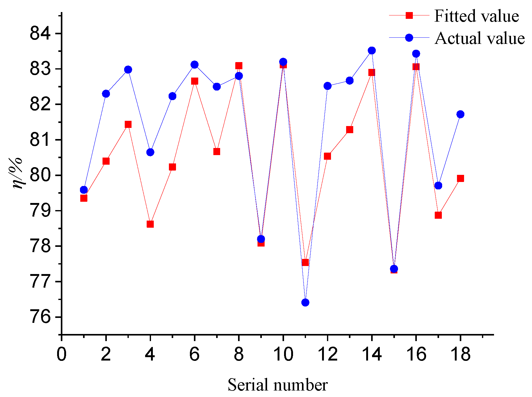
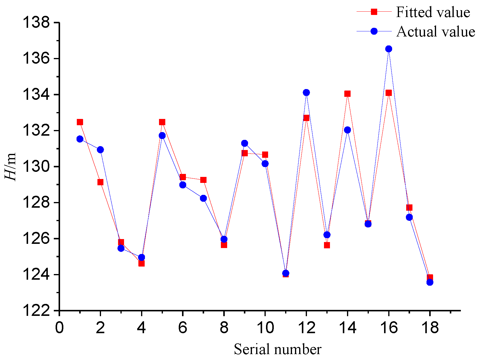
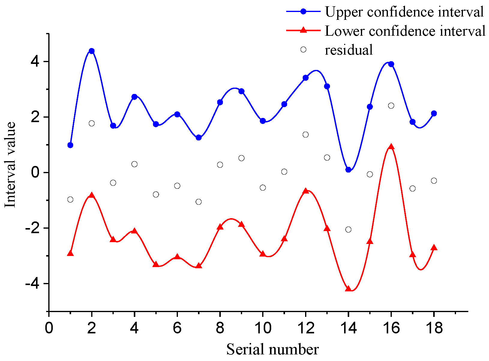
Since the difference test met the requirements, the fitting degree of the regression model was further analyzed by drawing the curve between the fitting value and the actual value as well as the residual confidence interval distribution graph. It can be seen from Figure 3 that the fitted value curve and the actual value curve have a high degree of coincidence in most of the intervals. The deviation of the two curves was very small, and only a few parameter combination points have large deviations. The fitting degree between the two curves was satisfied within the allowable error range for the orthogonal experimental model. 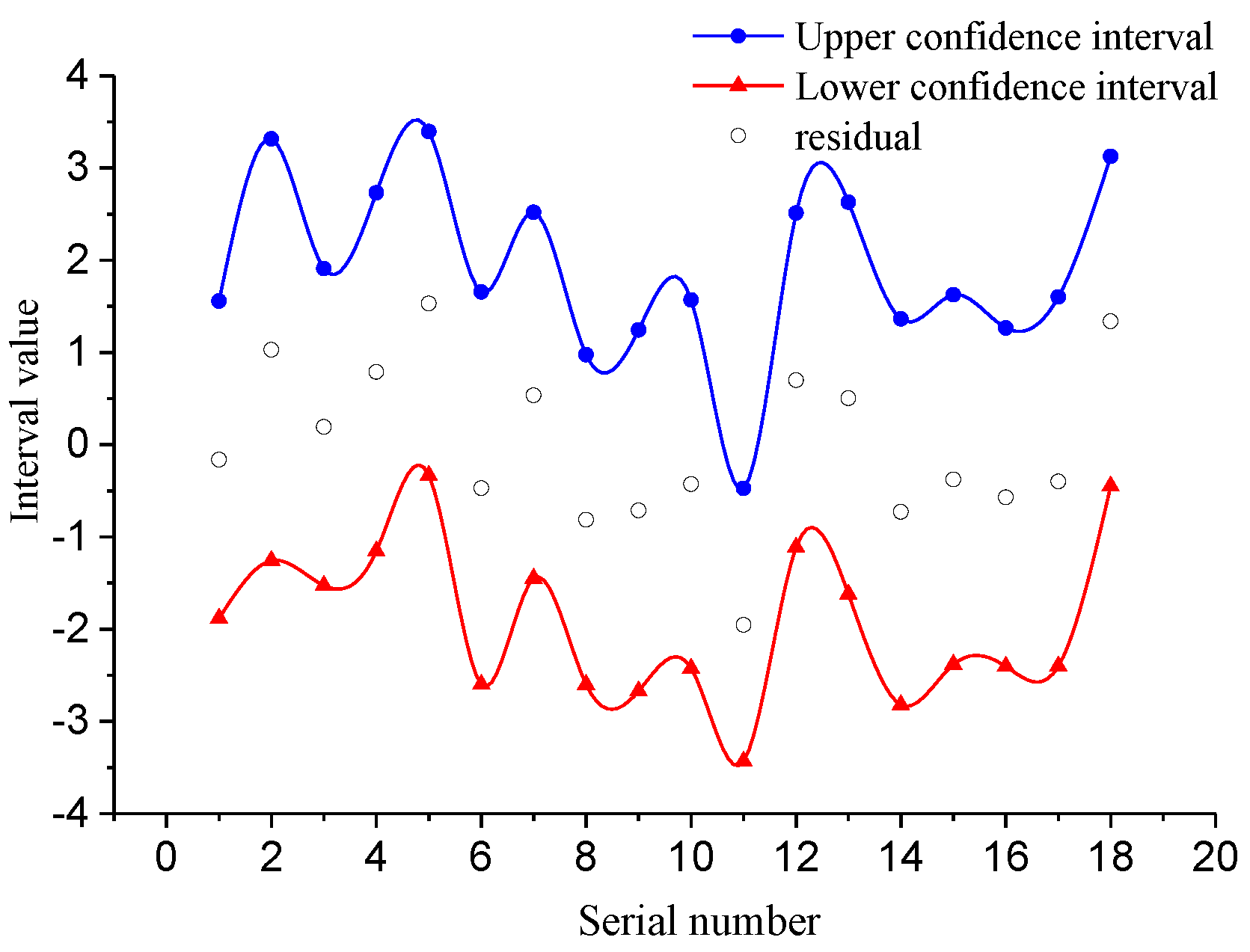It can be seen from Figure 4 that all residual values are within the upper and lower limits of the confidence interval, indicating that the regression model is normal.

According to the above operation, the corresponding command line was input to solve the mathematical regression model of the head and the geometric parameters of the different guide. The final output is as follows: the regression coefficients obtained are b₀ = 123.176, b₁ = −0.073, b₂ = −0.3085, b₃ = 0.221, b₄ = −0.0189, b₅ = −0.783, b₆ = 0.0185, r² = 0.9131, significant test statistics F = 19.2651, and the probability p = 0.064 corresponding to F value. It was indicated that the correlation coefficient (r² > 0.9) shows a strong correlation with a significant level (p > 0.05). Therefore, the regression model shows a positive significance. The regression coefficient range is shown in

Table 5. Regression coefficient Interval.

bi		bint
b0	123.176	[93.5186,152.8324]
b1	−0.073	[−0.2845,0.1385]
b2	−0.3085	[−0.7315,0.1145]
b3	0.221	[0.0523,0.3906]
b4	−0.0189	[−0.1881,0.1502]
b5	−0.783	[−0.9523,-0.6142]
b6	0.0185	[−0.0661,0.1031]

.

The regression model formula for the head of the reactor coolant pump is as follows:

H = 123.176 − 0.073α₃ − 0.3085α₄ + 0.221φ − 0.0189δ − 0.783R_t + 0.0185b₄.

(18)

It can be seen from the comparison between the fitting value and the actual value curve in Figure 5 that the coincidence degree between the fitting value curve (red line) and the actual value curve (blue line) is very high. The deviation value between the two is less than 1%, by which a very good fitting degree of the regression model was inculcated. It can also be seen from Figure 6 that the residual values are all within the confidence interval, indicating a normal regression model.

According to the above formula, the relationship between the geometric parameters of the guide vane and the idling speed and idling flow under the idling operation condition was derived. The established mathematical model of the idling speed is shown in Formula (19):

$$\{\begin{array}{l}N(t)=\frac{n_0}{1+\frac{g\rho Q_{0}H({\alpha }_3,{\alpha }_4,\delta ,R_t,b_4)}{4{\pi }^2{n}_e{}^{2}I\eta \left({\alpha }_3,{\alpha }_4,\delta ,R_t,b_4\right)}t}\\ \eta =54.061+0.0273a_3-0.256a_4+0.441f-0.092\delta -0.038R_t\\ H=123.176-0.073a_3-0.3085a_4+0.221f-0.0189\delta -0.783R_t+0.0185b_4\\ \\ 22\le a_3\le 30\\ 18\le a_4\le 22\\ 70\le \phi \le 80\\ 15\le \delta \le 25\\ 5\le R_t\le 15\\ 280\le b_4\le 300\end{array}$$

(19)

3.2. Test System of Reactor Coolant Pump Coasting

In order to verify the accuracy of the mathematical model of inertia, the open experiment table of the reactor coolant pump was built to complete the coasting test of the reactor coolant pump shut-down. The clear water was applied as the conveying medium of the experiment table system. The hydraulic characteristic, as well as the inertia-turn characteristic of the reactor coolant pump, was tested. The experiment table was designed to collect the instantaneous flow rate, the transient inlet, the outlet pressure and the instantaneous speed of the test pump in real-time. The experiment table was set as an open system test bench consisting of an idler wheel, motor, model pump, regulating valve, booster pump, pressure-stabilizing tank and measuring and collecting equipment (torque transducer, press transmitter, flow meter), and connecting pipes. Those were all listed in Figure 7, titled a test on the effect of model pump coasting behavior. The sectional flywheel was installed at the end of the shaft by means of key links. The control valve was adjusted to the maximum output. The model pump was opened to a certain period of stable operation and the control valve was adjusted to make the pump run stably under the condition of 1.0Q₀. The power supply was later turned off, and the variations of speed, flow, and head of the pump idleness transition process transmitted were observed by measuring and collecting equipment through the console computer for three tests.

In order to verify the universality of the model, the model of a group of guide vanes was established for experimental verification. Its main geometric parameters of guide vanes are concluded in

Table 6. Geometry parameter size of guide vanes.

Parameter	α3/°	α4/°	φ/°	δ/mm	Rt/mm	b4/mm
Value	24	18	78	22	6	296

. Meanwhile, the moment of inertia is I = 931 kg·m², and the parameters are substituted into Equation (19) to obtain the variation curve Equation (20) of the speed during the idling transition process under the corresponding guide vane parameters. The hydraulic performance test results of the reactor coolant pump are indicated in Figure 8.

$$N(t)=\frac{74}{3+1.2178t}\left(rad/s\right)$$

(20)

3.3. Verification of Mathematical Models

Based on the full characteristic curve of the pump combined with the test piping setup, the following factors are defined in the mathematical model of the test system: the water tank part pressure is represented by P₀; the pipe outlet to the model pump inlet section is represented by L1; the model pump outlet to the inlet of the water tank is represented by L2. The Q–H curve, Q–P curve, and the Q–η curve are fitted as polynomial equations, which are set as the system variables of the experimental mathematical model. The equation of fluid unsteady flow in the pressurized pipeline is combined with the principle of control process and rigid theory Equation (21) to establish the dynamic mathematical models (Equation (22)). As shown in Equation (22), the transient process of hydraulic change of the pump could be better reflected by this model when the pump was changed in a quasi-steady state under different working conditions. The model pump real-time flow Q and head H are defined in real-time by the input flow-head curve signal H(Q), while the input torque of the motor M_d is defined in real-time by the input flow-power curve signal P(Q). The resistance moment Mf is defined by both the input flow-torque curve signal P(Q) and the flow-efficiency curve signal slave η (Q). The mathematical model of pump speed is concluded in Formula (23):

$$\frac{1}{g}\frac{dQ}{dt}{{\displaystyle \int }}_0^L\frac{dx}{A}+\frac{v^2-v_1^2}{2g}+H-H_1+h_f=0$$

(21)

$$\begin{array}{l}{P}_1=P_0\rho g{H}_0-\rho \frac{L_1}{S_1}\frac{dQ}{dt}-\left({\lambda }_1\frac{L_1}{d_1}+{\xi }_1\right)\frac{\rho }{2S_1^2}{Q}^2-\rho g{L}_1\\ P_2=P_0\rho g{H}_0-\rho \frac{L_1}{S_1}\frac{dQ}{dt}-\left({\lambda }_2\frac{L_2}{d_2}+{\xi }_2\right)\frac{\rho }{2S_2^2}{Q}^2-\rho g{L}_1+\frac{\rho }{C_F^2}{Q}^2\\ H=\frac{P_2-P_1}{\rho g}\end{array}$$

(22)

$$\frac{d_n}{d_t}=\frac{30}{\pi J}\times \left(M_d-M_f\right)$$

(23)

where, P₁ and P₂ are defined as the inlet pressure and outlet pressure of the model pump respectively, Pa; P₀ is defined as the liquid level pressure of the tank, Pa; H₀ is defined as the level of the water tank, m; L₁ and L₂ are defined as length of inlet pipe and length of outlet pipe, respectively, m; S₁ and S₂ are defined as cross-sectional areas of the inlet pipe and outlet pipe, respectively, m². d₁ and d₂ are defined as pipe diameters of inlet pipe and outlet pipe, respectively, m; λ₁ and λ₂ are defined as the resistance coefficients of the inlet pipe and outlet pipe, respectively; ρ is defined as the fluid density, 1000 kg/m³; g is defined as the acceleration of gravity; Q is defined as the real-time flow rate of the model pump, m³/h; H is defined as the real-time head of the model pump, m; C_F is defined as the valve resistance coefficient; n is defined as the pump speed, r/min; J is defined as the moment of inertia of rotor parts, kg·m²; M_d is defined as the input torque of the motor, kg·m; M_f is defined as the resistance torque of the motor, kg·m; t is defined as the simulation process time, s.

In Formulas (22) and (23), the inertia of the experimental unit is indicated by J = 931 kg·m², while the pipe diameter and length are indicated by d₁ = d₂ = 0.76 m, L₁ = 20 m and L₂ = 30 m, respectively. The water tank liquid level pressure was indicated by P₀ = 1 atm and the water tank level is indicated by H₀ = 0.8 m. The starting speed of the motor is set as 1480 r/min and the mathematical model based on MATLAB was applied for the data output. The coasting output value of dQ/dt and dn/dt was obtained as 60 s while the flow rate and the speed curve of the corresponding time point were achieved by the integral operation. 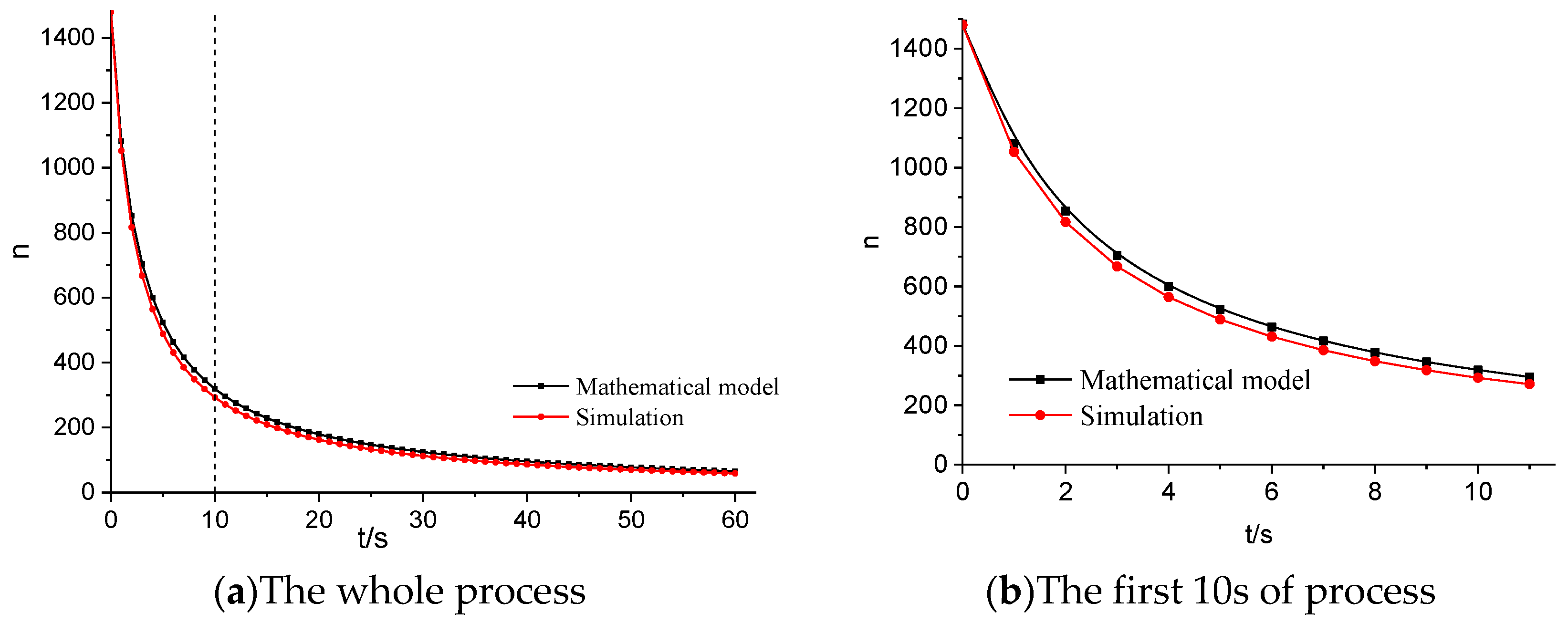The comparison between the test output coasting speed changes and the calculation results of the mathematical model coasting speed are indicated in Figure 9. It was shown that the trend of the rotational speed curve is similar to that of the 25 s while the error in the t = 10 s is approximately 2.7%, which is in the acceptable range. Therefore, the coasting rotational speed mathematical model is reliable for predicting the rotational speed of the coasting transition process.

4. Conclusions

(1) Benefiting from the mathematical derivation of the equilibrium equation of the nonlinear inertia transient process, the mathematical relationship between the rotational speed of the inertia transition process and the fixed head and the efficiency of the reactor coolant pump were obtained.

(2) The hydraulic model of 18 sets of different guide vane structure parameters was established under the orthogonal optimization scheme. Based on the multiple linear regression theory, the orthogonal test optimization results of the parameters of the guide vane were calculated by multiple regression analysis. At last, the mathematical relationship of the hydraulic performance of the guide vane parameters was predicted while the mathematical model on the main geometrical parameters of the given guide vane was deduced by the simultaneous mathematical relationship among the rotational speed, the fixed head and the efficiency of the reactor coolant pump.

(3) The mathematical model of coasting was verified by the test results and the speed curve of the idling transition process and the speed curve derived from the mathematical model were evidenced with a good coincidence degree, indicating that the coasting transition process can be well predicted by the constructed coasting model.

References

1. Sun, H. Third Generation Nuclear Power Technology AP1000, 2nd ed.; China Electric Power Press: Beijing, China, 2016. [Google Scholar]
2. Yanjun, W.; Wenhong, L.; Jun, D.; Ling, G. Comparison of past and present the Chernobyl and the Fukushima nuclear accident and elicit thinking. Chin. J. Radiol. Health 2016, 25, 459–462. [Google Scholar]
3. Dien, L.; Diep, D. Verification of VVER-1200 NPP simulator in normal operation and reactor coolant pump coast-down transient. World J. Eng. Technol. 2017, 5, 507–519. [Google Scholar] [CrossRef]
4. Turnbull, B. RELAP5/MOD3.3 analysis of the reactor coolant pump trip event at NPP Krško for different transient scenarios. In Proceedings of the International Conference Nuclear Energy for New Europe 2005, Bled, Slovenia, 5–8 September 2005. [Google Scholar]
5. Senru, Z. Calculation of transient characteristics for main circulating pump. Nuclear Power Eng. 1993, 2, 183–190. [Google Scholar]
6. Yujun, G.; Jinling, Z.; Huizheng, Q.; Guanghui, S.; Dounan, J.; Zhenwan, Y. Calculating model of coolant pump flow characteristics for reactor system. Nucl. Sci. Eng. 1995, 3, 220–225, 231. [Google Scholar]
7. Shaowen, D. Transient calculation of main pump in Qinshan Nuclear Power Plant Phase Two Project. Nucl. Power Eng. 2001, 6, 494–496, 507. [Google Scholar]
8. Xu, Y. Numerical Simulation of Interior Flow Field of Reactor Coolant Pump Under Station Blackout Accident; Dalian University of Technology: Dalian, China, 2011. [Google Scholar]
9. Zhu, R.; Long, Y.; Fu, Q.; Yuan, S.; Wang, X. Pressure fluctuation characteristics of nuclear main pump under low flow conditions. J. Vibr. Shock 2014, 33, 143–149. [Google Scholar]
10. Yun, L.; Zhu, R.; Fu, Q.; Yuan, S.; Xi, Y. Numerical analysis on unstable flow of reactor coolant pump under small flow rate condition. J. Drain. Irrig. Eng. 2014, 32, 290–295. [Google Scholar]
11. Feng, X.; Wu, D.; Yang, L.; Jia, Y. CNP1000 shaft seal reactor coolant pump technology. J. Drain. Irrig. Mach. Eng. 2016, 34, 553–560. [Google Scholar]
12. Alatrash, Y.; Kang, H.O.; Yoon, H.G.; Seo, K.; Chi, D.Y.; Yoon, J. Experimental and analytical investigations of primary coolant pump coastdown phenomena for the Jordan Research and Training Reactor. Nucl. Eng. Des. 2015, 286, 60–66. [Google Scholar] [CrossRef]
13. Brady, D.R.; Loebig, T.G. Reactor Coolant Pump Motor Load-Bearing Assembly Configuration. U.S. Patent No. 9,273,694, 1 March 2016. [Google Scholar]
14. Bang, S.Y.; Chu, S.M.; Chang, J.Y. Development of Reactor Coolant Pump for APR1400. In Proceedings of the KNS 2015 Fall Meeting, Kyungju, Korea, 28–30 October 2015. [Google Scholar]
15. Metzroth, K.; Denning, R.; Aldemir, T. Dynamic Event Tree Modeling of a Reactor Coolant Pump Seal LOCA. Adv. Conc. Nucl. Energy Risk Assess. Manag. 2018, 1, 305. [Google Scholar]
16. Lu, Y.; Zhu, R.; Fu, Q.; Fu, Q.; An, C.; Chen, J. Research on the structure design of the LBE reactor coolant pump in the lead base heap. Nucl. Eng. Technol. 2019, 51, 546–555. [Google Scholar] [CrossRef]
17. Lu, Y.; Zhu, R.; Wang, X.; Yang, W.; Qiang, F.; Daoxing, Y. Study on the complete rotational characteristic of coolant pump in the gas-liquid two-phase operating condition. Ann. Nucl. Energy 2019, 123, 180–189. [Google Scholar]
18. Lu, Y.; Zhu, R.; Wang, X.; An, C.; Zhao, Y.; Fu, Q. Experimental study on transient performance in the coasting transition process of shutdown for reactor coolant pump. Nucl. Eng. Des. 2019, 346, 192–199. [Google Scholar] [CrossRef]
Figure 1. Main structural parameters of the guide vane.
Processes 07 00452 g001
Figure 2. The water model and grid diagram of the reactor coolant pump.
Processes 07 00452 g002
Figure 3. Comparison of fitted value and actual value for efficiency.
Processes 07 00452 g003
Figure 4. Residual confidence interval.
Processes 07 00452 g004
Figure 5. Comparison of fitted value and actual value for the head.
Processes 07 00452 g005
Figure 6. Residual confidence interval.
Processes 07 00452 g006
Figure 7. Site of the experiment table system.
Processes 07 00452 g007
Figure 8. Numerical results of the reactor coolant pump.
Processes 07 00452 g008
Figure 9. Chart of simulation test and mathematical model calculation results.
Processes 07 00452 g009