A Lagrangian Particle Algorithm (SPH) for an Autocatalytic Reaction Model with Multicomponent Reactants

Abstract

For the numerical simulation of convection-dominated reacting flow problems governed by convection-reaction equations, grids-based Eulerian methods may cause different degrees of either numerical dissipation or unphysical oscillations. In this paper, a Lagrangian particle algorithm based on the smoothed particle hydrodynamics (SPH) method is proposed for convection-reaction equations and is applied to an autocatalytic reaction model with multicomponent reactants. Four typical Eulerian methods are also presented for comparison, including the high-resolution technique with the Superbee flux limiter, which has been considered to be the most appropriate technique for solving convection-reaction equations. Numerical results demonstrated that when comparing with traditional first- and second-order schemes and the high-resolution technique, the present Lagrangian particle algorithm has better numerical accuracy. It can correctly track the moving steep fronts without suffering from numerical diffusion and spurious oscillations.

1. Introduction

Reacting flow models play an important role in the simulation of many physical and engineering problems, such as the pollutant transport process in water and air, heat conduction process in flowing fluids, chromatography column in reactors [1], and high-speed eddy current in electromagnetic fields [2]. A reacting flow model is often composed of a group of convection dominated partial differential equations (PDEs) with non-linear source terms [2,3,4,5], which usually accompanies autocatalytic reactions. Through mutation, the automatic catalyst is transformed into another form, which can simultaneously conduct autocatalytic reaction and ultimately result in competition between the palingenetic and original automatic catalyst [6]. By accurately solving these reacting flow models, we can not only analyze the reaction problems in chemistry, physics, electromagnetics and fluids, but can also design proper reaction units and optimize the schemes for process control. Therefore, developing an accurate and efficient numerical method is of great significance to promote the development of these disciplines.

The PDEs in reacting flow models are usually convection dominated, i.e., the transport of reactants is more affected by the flow than the diffusion and reaction processes, and the time scale for convection is smaller than those for diffusion and reaction [7]. It is well known that convection dominated PDEs present various difficulties to numerical methods, especially when discontinuities or moving steep fronts are presented [1,7,8]. In order to clearly observe the differences among different discretization schemes, Lim et al. [1] reviewed fourteen competitive spatial discretization methods developed for convection terms and analyzed their accuracy, temporal performance and stability. The discretization methods were classified by fixed stencil (traditional upwind and central schemes), adaptive stencil (ENO (essentially non-oscillatory) schemes) and weighted stencil (weight ENO (WENO) schemes) types. It is found that the ENO and WENO methods are efficient for tracking a shock because they avoid crossing discontinuities in the interpolation procedure with a relatively small number of mesh points, thus they are generally considered to be the most powerful tools for convection dominated problems. Wang and Hutter [4] compared a series of numerical schemes for one-dimensional convection-diffusion problems and Alhuamaizi [7] gave a comparative evaluation of different finite difference methods for a convection-dominated reaction problem with three reactants. The evaluated methods include first-order accurate difference schemes like upstream difference (well-known as upwind) and Lax-Friedrichs, second-order methods like central, Lax-Wendroff, Fromm and Beam-Warming, third-order upwind and QUICK, and the high-resolution techniques, including the total variation diminishing (TVD) methods with flux-limiters, flux-corrected transport (FCT), monotone upstream scheme for conservation laws (MUSCL) and WENO. Numerical experiments have well proved that first-order accurate solutions are likely to produce unacceptable numerical diffusion, while higher order numerical methods easily result in unphysical oscillation (Gibbs phenomena) with various levels of accuracy loss [4,7]. By increasing the grid number and hence decreasing the grid Peclet number in first-order methods, numerical diffusion can be resolved, but high computational costs will be caused in the process. Wang and Hutter [4] pointed out that the modified TVD Lax-Friedrichs scheme with the Superbee limiter [9,10,11] (MTVDLF-Superbee) is the most competent method for convection dominated problems with a steep spatial gradient of the variables. Alhuamaizi [7] concluded that high-resolution techniques such as FCT, MUSCL and WENO schemes and TVD with flux limiters, are all efficient for tracking steep moving fronts and are essential for cases which use small numbers of grid points. In terms of both accuracy and computing time, the Superbee flux limiter is found to be the most appropriate method for simulating the sharp fronts of the reactor model.

All of the above numerical methods are based on the finite difference or finite volume discretization, which belong to Eulerian approaches using grids fixed in space. Grid-based high-resolution approaches can eliminate excessive numerical diffusion without causing unphysical oscillations, but they can hardly deal well with numerical accuracy and computational efficiency at the same time, and hence are not suitable for long-term and large-scale transport processes with multicomponent reactants. In addition, the implementation process is somewhat tedious and involves many intermediate variables. The objective of this paper is to develop a Lagrangian particle algorithm based on a smoothed particle hydrodynamics (SPH) method for convection-reaction equations to enhance both the numerical accuracy and computational efficiency.

Smoothed particle hydrodynamics is a fully Lagrangian, or meshless particle method invented in the late 1970s by Lucy [12] and Gingold and Monaghan [13] to solve unbounded astrophysical flow problems. The basic idea of the method is to represent a continuous fluid with a group of interacting particles, each of which carries various physical quantities such as mass, density, position, velocity, concentration, etc. It consists two steps of approximation known as kernel approximation and particle approximation [14]. As a build-in feature of the SPH method, the adaptive nature makes it very attractive and it can easily handle problems involving large deformations and highly irregular geometries. In principle, as long as the number of particles is sufficient and the particle distribution is not too irregular, the approximations will be accurate and the process can be properly described. On the basic theory of SPH, the readers are referred to the recent reviews [15,16,17,18,19].

Regarding to the application of SPH to transport problems, Gadian et al. [20] used SPH to extend the developments in finite difference and finite-element to the modelling of atmospheric fluid flow. The particle method was used to describe the 2D convection. Zhu and Fox [21] presented the application of SPH to tracer diffusion in porous media under steady state and transient conditions. Based on the multiphase SPH framework, Adami et al. [22] proposed a Lagrangian particle method for the simulation of multiphase flows with surfactant. The insoluble surfactant on an arbitrary interface geometry as well as interfacial transport such as adsorption or desorption were simulated. Szewc et al. [23] proposed a new variant of SPH for the simulation of natural convection phenomena in a non-Boussinesq regime. Orthmann and Kolb [24] applied SPH to convection-diffusion simulations of incompressible fluids. A temporal blending technique was proposed to reduce the number of particles in the simulation. It greatly reduced the error introduced in the pressure term when changing particle configurations and enabled larger integration time-steps in the transition phase. Using SPH as a discretization tool on uniform Eulerian grids, Danis et al. [25] investigated transient and laminar natural convection in a square cavity. To obtain a divergence-free velocity field, the incompressibility was strictly enforced by employing a pressure projection method. Although the SPH method has been successfully applied to simulate transport processes, it is mainly used for solving fluid dynamics with a focus on capturing the free-surface and moving interface [15,18,22]. Its application to diffusion is restricted to the transport process in porous media [21], where the flow velocity is relatively slow.

To show the advantages of the proposed Lagrangian particle algorithm, its numerical results and computational performance are compared with those of four typical Eulerian methods, including the upstream difference scheme (UDS), Lax- Friedrichs scheme (LFS), Lax-Wendroff scheme (LWS) and MTVDLF-Superbee method.

The structure of this paper is organized as follows. The reacting flow model governed by the one-dimensional convection-reaction equations is introduced in Section 2. Traditional Eulerian methods including UDS, LFS, LWS and MTVDLF-Superbee are presented in Section 3. Section 4 describes the Lagrangian particle algorithm (SPH) and its application to the autocatalytic reaction model with multicomponent reactants. Numerical results are presented in Section 5 with detailed comparison between the proposed Lagrangian particle scheme and the Eulerian methods. Finally, some discussions and concluding remarks are drawn in Section 6.

2. Reacting Flow Model

2.1. Convection-Reaction Equations

Considering the chemical reaction process, the mathematical model describing the transport process of the reactants is governed by the following one-dimensional convection-diffusion-reaction equation:

$$\frac{\partial U}{\partial t}+a\frac{\partial U}{\partial x}=\frac{\partial }{\partial x}\left(\epsilon \frac{\partial U}{\partial x}\right)+G\left(U\right)$$

(1)

where $U$ represents the reactant concentration, which is a scalar for single component reactant, and a vector for multicomponent reactants, $x$ and $t$ are spatial and time coordinates respectively, $a$ is the velocity of the flow, and $\epsilon$ denotes the diffusion coefficient of the reactant in the fluid, $G\left(U\right)$ represents the reaction source term, which is determined by the specific reaction flow model. Note that $a$ and $\epsilon$ are both considered to be positive constant values.

According to the time scale of convection, diffusion and reaction process, the whole transport process can be divided into convection dominated, diffusion dominated, and reaction dominated problems [8]. For the general catalytic problems, the diffusion process is relatively slow and hence is often ignored. Therefore, the transport of reactants is changed into a convection-reaction problem, and the mathematical model (1) is simplified to:

$$\frac{\partial U}{\partial t}+a\frac{\partial U}{\partial x}=G\left(U\right)$$

(2)

or in the conservation form

$$\frac{\partial U}{\partial t}+\frac{\partial f\left(U\right)}{\partial x}=G\left(U\right)$$

(3)

where $f\left(U\right)=aU$ is the convective flux.

2.2. Autocatalytic Reaction Model

In this work, we considered a widely used autocatalytic reaction model proposed by Alhumaizi et al. [7], which takes place in a tubular reactor. The reaction model contains three component reactants denoted by A, B and C, and it consists of the following steps:

• Replication of reactant B: $A+2B\stackrel{k_1}{\to }3B$
• Death of reactant B: $B\stackrel{k_2}{\to }{P}_1$
• Mutation of reactant B into reactant C: $A+2B\stackrel{\alpha k_1}{\to }2C+B$
• Replication of reactant C: $A+2C\stackrel{\beta k_1}{\to }3C$
• Death of reactant C: $C\stackrel{k_2/\beta }{\to }{P}_2$

where the parameters $k_1$ and $k_2$ represent the rate constants, $\alpha$ is the mutation constant and $\beta$ is the mutation efficiency. For simplification, a constant flow velocity along the reactor is assumed.

The governing equations for the transport of three reacting species written in dimensionless form are expressed as:

$$\mathrm{For}\mathrm{A}:\frac{\partial U_1}{\partial T}+V\frac{\partial U_1}{\partial X}=\left(1-U_1\right)\left[\left(1+\alpha \right)U_2^2+\beta U_3^2\right]$$

(4)

$$\mathrm{For}\mathrm{B}:\frac{\partial U_2}{\partial T}+V\frac{\partial U_2}{\partial X}=\left(1-U_1\right)\left(1-\alpha \right)U_2^2-\gamma U_2$$

(5)

$$\mathrm{For}\mathrm{C}:\frac{\partial U_3}{\partial T}+V\frac{\partial U_3}{\partial X}=\left(1-U_1\right)\left(\beta U_3^2+2\alpha U_2^2\right)-\frac{\gamma }{\beta }{U}_3$$

(6)

where the dimensionless concentration $U_i\left(i=1,2,3\right)$ of species A, B, C and other dimensionless parameters are formulated as

$$U_1=\frac{u_f-u_1}{u_f},U_2=\frac{u_2}{u_f},U_3=\frac{u_3}{u_f},X=\frac{x}{L},T=k_1{u}_f^{2}t,V=\frac{a}{k_1{u}_f^{2}L},\gamma =\frac{k_2}{k_1{u}_f^2}$$

(7)

where $u_i\left(i=1,2,3\right)$ represent the concentration of reacting species A, B, C before nondimensionalization, $x$ is the spatial coordinate and $t$ is the time, $u_f$ is the feed substrate concentration and $L$ represents the length of the tubular reactor.

The system equations are closed together with the initial conditions

$$U_1\left(X,0\right)=1,U_2\left(X,0\right)=0,U_3\left(X,0\right)=0$$

(8)

and the boundary conditions

$$U_1\left(0,T\right)=0,U_2\left(0,T\right)=1,U_3\left(0,T\right)=0$$

(9)

$$U_1\left(1,T\right)=1,U_2\left(1,T\right)=0,U_3\left(1,T\right)=0$$

(10)

which are Dirichlet boundary conditions imposed at the inlet and outlet of the tubular reactor. Equation (10) implies that the reaction process has not arrived at the outlet boundary within the simulation time.

3. Traditional Eulerian Methods

Many numerical methods have been applied to the convection-reaction equations. The finite difference and finite element methods are more classical, but the finite volume methods (FVMs) [26] are more widely used due to their conservative properties. The basic strategy of FVMs is to write the differential equation in conservation form, integrate it over small regions (called “cells” or “finite volumes”) and convert each such integral into an integral over the boundary of the cell by means of the divergence theorem.

Common schemes of FVMs for convection-reaction equations include the first-order accurate methods like the upwind and Lax-Friedrichs (LF) schemes, the second-order accurate methods, such as the second order upwind, Lax-Wendroff, Beam-Warming and Fromm schemes, and the high-order accurate QUICK and the modified TVD Lax-Friedrichs scheme with different slope limiters [2,7,8]. To better compare and analyze the numerical performance of the proposed Lagrangian particle algorithm, four typical Eulerian methods are studied as the comparisons.

By discretizing the spatial and temporal derivatives in Equation (3) using the finite volume method, we obtained

$$U_j^{n+1}=U_j^n-\frac{\Delta t}{\Delta x}\left(F_{j+1/2}-F_{j-1/2}\right)+\Delta tG\left(U_j^n\right)$$

(11)

where $F_{j\pm 1/2}$ are the numerical fluxes on the cell interfaces at $x_{j\pm 1/2}$, and $\Delta t$ and $\Delta x$ are the time and space step size, respectively. Mean value theorem is applied to the reaction term $G\left(U\right)$. Many schemes have been developed and the difference between them just depends on how to define the numerical convective fluxes.

The convective flux of the upwind scheme is given by

$$F_{j+1/2}^n=\frac{1}{2}\left(f_{j+1}^n+f_j^n-{\phi }_{j+1/2}^n\right)$$

(12)

with $f_j^n=f\left(U_j^n\right)$, ${\phi }_{j+1/2}^n=\left|a_{j+1/2}^n\right|\Delta U_{j+1/2}^n$ and $\Delta U_{j+1/2}^n=U_j^{n+1}-U_j^n$. The characteristic velocity $a_{j+1/2}^n$ is given by

$$a_{j+1/2}^n=\{\begin{array}{c}\frac{\left(f_{j+1}^n-f_j^n\right)}{\Delta U_{j+1/2}^n},\Delta U_{j+1/2}^n\ne 0\\ a,\Delta U_{j+1/2}^n=0\end{array}$$

(13)

The convective flux of the Lax-Friedrichs scheme is

$$F_{j+1/2}^n=\frac{1}{2}\left(f_{j+1}^n+f_j^n-\frac{\Delta x}{\Delta t}\left(U_{j+1}^n-U_j^n\right)\right)$$

(14)

The upwind and LFS are first-order accurate in both space and time.

The convective flux of the Lax-Wendroff scheme (LWS) is based on Taylor series expansion of the space derivative term [5,27] and can be written as

$$F_{j+1/2}^n=f\left(U_{j+1/2}^n\right)\mathrm{with}{U}_{j+1/2}^n=\frac{1}{2}\left(U_{j+1}^n+U_j^n\right)-\frac{\Delta t}{2\Delta x}\left(f_{j+1}^n-f_j^n\right)$$

(15)

This scheme has second-order accuracy in both space and time.

In the modified TVD Lax-Friedichs (MTVDLF) scheme, the convective flux is given by

$$F_{j+1/2}=\frac{1}{2}\left(f\left(U_{j+1/2}^R\right)+f\left(U_{j+1/2}^L\right)-{\phi }_{j+1/2}^{MTVDLF}\right)$$

(16)

and the modified dissipative limiter [28] is

$${\phi }_{j+1/2}^{MTVDLF}={\left|a_{j+1/2}^{RL}\right|}_{max}\left(U_{j+1/2}^R-U_{j+1/2}^L\right)$$

(17)

where the characteristic speed $a_{j+1/2}^{RL}$ is obtained from the Rankine-Hugoniot jump condition

$$a_{j+1/2}^{RL}=\{\begin{array}{c}\frac{f\left(U_{j+1/2}^R\right)-f\left(U_{j+1/2}^L\right)}{U_{j+1/2}^R-U_{j+1/2}^L},\mathrm{if} U_{j+1/2}^R\ne U_{j+1/2}^L\\ a{U}_{j+1/2},\mathrm{if}{U}_{j+1/2}^R=U_{j+1/2}^L\end{array}$$

(18)

and $U_{j+1/2}^L$ and $U_{j+1/2}^R$ have been considered to form a linear piecewise reconstruction for each interface. The former is obtained from the left-side cell $U_j$ and the latter is due to the right-side cell $U_{j+1}$. The specific expressions are

$$U_{j+1/2}^L=U_j+\frac{1}{2}\Delta x{\sigma }_j,U_{j+1/2}^R=U_{j+1}-\frac{1}{2}\Delta x{\sigma }_{j+1}$$

(19)

where the slop limiter is defined as ${\sigma }_j={\varphi }_j\left(U_{j+1}-U_j\right)/\Delta x$ and ${\varphi }_j$ is a function of ${\theta }_j$, which represents the ratio of the consecutive gradients, i.e.,

$${\varphi }_j=\varphi \left({\theta }_j\right),{\theta }_j=\frac{U_j-U_{j-1}}{U_{j+1}-U_j}$$

(20)

There are various choices for the function $\varphi \left(\theta \right)$ in practice [29]. If $\varphi \left(\theta \right)$ is defined by the upper boundary of the second-order TVD region, the so-called Superbee limiter [4,29] is resulted as

$${\varphi }^{Superbee}\left(\theta \right)=\mathit{max}\left(0,\mathit{min}\left(1,2\theta \right),\mathit{min}\left(\theta ,2\right)\right)$$

(21)

4. Lagrangian Particle Algorithm (SPH)

The smoothed particle hydrodynamics (SPH) method [30,31] has been well-known in fluid simulation problems since its proposition by Lucy [12] and Gingold and Monaghan [13]. It is a fully Lagrangian, meshless method in which an approximation technique with a smoothing kernel function is introduced to estimate the spatial derivatives in the governing equations of fluid dynamics. Different from traditional mesh-based methods, the SPH method uses a set of particles without predefined connectivity. It simulates complex flow-related problems by solving the hydrodynamic equations and tracking the particle trajectories. Each particle has characteristic properties of mass, density, velocity, position and others, depending on the specific problem. In the light of mesh independence among individual particles, the number of particles in the calculation domain can be increased or decreased to satisfy the solution requirements for complex problems.

Regarding to the basic idea, there are two main steps in the SPH method, namely, kernel approximation and particle approximation, which are presented in this section.

4.1. SPH Kernel Approximation

The integral representation for any physical quantity $f\left(x\right)$ can be written as

$$f\left(x\right)=\underset{\mathsf{\Omega }}{\overset{}{{\displaystyle \int }}}f\left(x^{\prime }\right)\delta \left(x-x^{\prime }\right)d{x}^{\prime }$$

(22)

where $\mathsf{\Omega }$ is the domain containing x and $\delta \left(x-x^{\prime }\right)$ is the Dirac delta function defined as

$$\delta \left(x-x^{\prime }\right)=\{\begin{array}{c}1,x=x’\\ 0,x\ne x’\end{array}$$

Replacing $\delta \left(x-x^{\prime }\right)$ by a kernel function $W=W\left(x-x^{\prime },h\right)$, then Equation (22) can be converted into the SPH kernel approximation form as

$$⟨f\left(x\right)⟩=\underset{\mathsf{\Omega }}{\overset{}{{\displaystyle \int }}}f\left(x^{\prime }\right)W\left(x-x^{\prime },h\right)d{x}^{\prime }$$

(23)

where $⟨\cdot ⟩$ represents the value approximation, $h$ is known as the smoothing length and it determines the radius of the compact support of $W$. The kernel $W$ should satisfy the following requirements:

(i)

normalization condition: ${{\displaystyle \int }}_{\mathsf{\Omega }}^{}W\left(x-x^{\prime },h\right)d{x}^{\prime }=1$;

(ii)

compact support: $W\left(x-x^{\prime },h\right)=0$, if $\left|x-x^{\prime }\right|>\kappa h$, where $\kappa$ is a scale parameter and $\kappa h$ is called nuclear radius;

(iii)

nonnegativity: $W\left(x-x^{\prime },h\right)\ge 0$, if $\left|x-x^{\prime }\right|\le \kappa h$;

(iv)

symmetry: $W\left(x-x^{\prime },h\right)=W\left(x’-x,h\right)$;

(v)

monotone decline: $W$ is monotonically decreasing with respect to $\left|x-x^{\prime }\right|$, which represents decreasing interaction;

(vi)

Dirac delta function property: $\underset{h\to 0}{\lim }W\left(x-x^{\prime },h\right)=\delta \left(x’-x\right)$.

The step of kernel approximation is equivalent to the smoothing and denoising of the original signal.

In order to obtain the approximation of the derivative of a function, we used $\nabla f\left(x\right)$ to replace $f\left(x\right)$ in Equation (23) and get

$$⟨{\nabla }_{x}f\left(x\right)⟩=\underset{\mathsf{\Omega }}{\overset{}{{\displaystyle \int }}}\left[{\nabla }_{x^{\prime }}f\left(x^{\prime }\right)\right]W\left(x-x^{\prime },h\right)d{x}^{\prime }$$

(24)

where $\nabla$ is the gradient operator. According to the divergence theorem, (24) can be transformed into

$$⟨{\nabla }_{x}f\left(x\right)⟩=\underset{\mathsf{\Omega }}{\overset{}{{\displaystyle \int }}}{\nabla }_{x^{\prime }}\left[f\left(x^{\prime }\right)W\left(x-x^{\prime },h\right)\right]d{x}^{\prime }-\underset{\mathsf{\Omega }}{\overset{}{{\displaystyle \int }}}f\left(x^{\prime }\right){\nabla }_{x^{\prime }}W\left(x-x^{\prime },h\right)d{x}^{\prime }$$

(25)

Using the compact support property of the kernel, when the support domain of $W$ was located inside the problem domain, we obtained ${{\displaystyle \int }}_{\mathsf{\Omega }}^{}{\nabla }_x·\left[f\left(x^{\prime }\right)W\left(x-x^{\prime },h\right)\right]d{x}^{\prime }=0$. Therefore, for a point with kernel support in the problem domain, formulation (25) can be written as

$$⟨{\nabla }_{x}f\left(x\right)⟩=-\underset{\mathsf{\Omega }}{\overset{}{{\displaystyle \int }}}f\left(x^{\prime }\right){\nabla }_{x^{\prime }}W\left(x-x^{\prime },h\right)d{x}^{\prime }=\underset{\mathsf{\Omega }}{\overset{}{{\displaystyle \int }}}f\left(x^{\prime }\right){\nabla }_{x}W\left(x-x^{\prime },h\right)d{x}^{\prime }$$

(26)

which is the standard expression for the derivative approximation in SPH.

4.2. SPH Particle Approximation

In the particle algorithm, the continuum medium was partitioned into a finite number of $N$ parts that are referred to as particles. Particle approximation is a process of transforming the integral in kernel approximation into a discrete summation form of particles in the support domain. Each particle carries a mass, density, velocity, concentration, and other properties depending on the specific problem. Here using $\Delta V_j$ to represent the volume of particle $j$, then its mass can be calculated by

$$m_j=\Delta V_j{\rho }_j$$

(27)

where ${\rho }_j$ is the density of particle $j$.

Applying particle approximation to the integrals in kernel approximations (23) and (26), the SPH approximation of $f\left(x\right)$ at $x_i$ can be written as

$$⟨f\left(x_i\right)⟩={\displaystyle \sum }_{j=1}^{N}f\left(x_j\right)W\left(x_i-x_j,h\right)\frac{m_j}{{\rho }_j}$$

(28)

and the SPH approximation of the derivatives can be obtained as

$$⟨\nabla f\left(x_i\right)⟩={\displaystyle \sum }_{j=1}^{N}f\left(x_j\right){\nabla }_{i}W\left(x_i-x_j,h\right)\frac{m_j}{{\rho }_j}$$

(29)

With the anti-symmetry property of the kernel gradient, i.e., ${{\displaystyle \sum }}_{j=1}^N{\nabla }_{i}W\left(x_i-x_j,h\right)\frac{m_j}{{\rho }_j}=0$, we can obtain the mostly used derivative approximation in SPH as

$$⟨\nabla f\left(x_i\right)⟩={\displaystyle \sum }_{j=1}^N\left[f\left(x_j\right)-f\left(x_i\right)\right]{\nabla }_{i}W\left(x_i-x_j,h\right)\frac{m_j}{{\rho }_j}$$

(30)

or simply

$$⟨\nabla f_i⟩={\displaystyle \sum }_{j=1}^N\frac{m_j}{{\rho }_j}(f_j-f_i){\nabla }_i{W}_{ij}$$

(31)

where $f_i=f\left(x_i\right)$, ${\nabla }_i{W}_{ij}=\frac{\partial W\left(\left|x_i-x_j\right|,h_i\right)}{\partial x_i}=\frac{\partial W_{ij}}{\partial x_i}$, which denotes the kernel derivatives taken with respect to the coordinates of particle $i$ and $h_i$ is the smoothing length of particle $i$.

4.3. Lagrangian Particle Autocatalytic Reaction Model

With the definition of material derivative, the convection-reaction equation (2) can be written in Lagrangian form as

$$\frac{dU}{dt}=G\left(U\right)$$

(32)

$$\frac{dx}{dt}=a$$

(33)

Applying the SPH approximation to Equation (32), we get

$$\frac{d{U}_i}{dt}={\displaystyle \sum }_{j=1}^{N}G\left(U_i\right)W\left(x_i-x_j,h\right)\frac{m_j}{{\rho }_j}$$

(34)

Contrary to Euler approaches that use fixed grids in space, in the Lagrangian particle scheme, the particles move according to the flow velocity

$$\frac{d{x}_i}{dt}={\displaystyle \sum }_{j=1}^N{a}_{i}W\left(x_i-x_j,h\right)\frac{m_j}{{\rho }_j}$$

(35)

With a time integration algorithm, the semi-discrete formulations of the Lagrangian convection-reaction Equation (34) and the particle motion (35) can be marched until the specified simulation time. For simplicity, the explicit Euler method is applied in this paper, which is one-step and first-order accurate.

Since the location of each particle changes with time, adding particles at the inlet and deleting particles at the outlet is required to mimic the flowing medium. A new particle is added when the most leftmost particle gets across the inlet boundary, and a particle is deleted when it gets across the outlet boundary. It is worth noting that at most one particle needs to be added at one time step for the one-dimensional reaction problem considered herein. This condition is equivalent to the CFL condition in grid based methods and it must be satisfied to ensure the continuity of the flowing medium.

5. Numerical Results

In this paper, the kinetic parameters in the autocatalytic reaction model were taken as $\alpha =0.065$, $\beta =2.0$ and $\gamma =0.025$, and the dimensionless flow velocity is $V=1.0$. These parameters have been well studied by Alhumaizi [7]. In all the following simulations, $\Delta t=0.0002$ is taken as the time step size. The space step size is $\Delta x=1/N$, where N denotes the number of particles for Lagrangian particle method and grid points for grid-based methods.

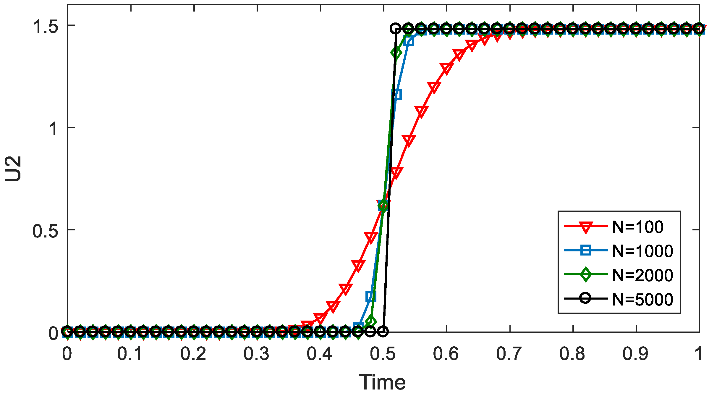
The concentration of species B at $X=0.5$ simulated by the upwind scheme (UDS) with different grid numbers is shown in Figure 1. It is seen that with an increased grid number the UDS results converge to a particular solution, which is similar to the conclusion that the limitation of UDS for solving convection-diffusion equation converges to the theoretical solution [3]. Since there is no exact solution for the autocatalytic reaction model considered herein, the UDS solution with grid number $N=5000$ is taken as the reference.

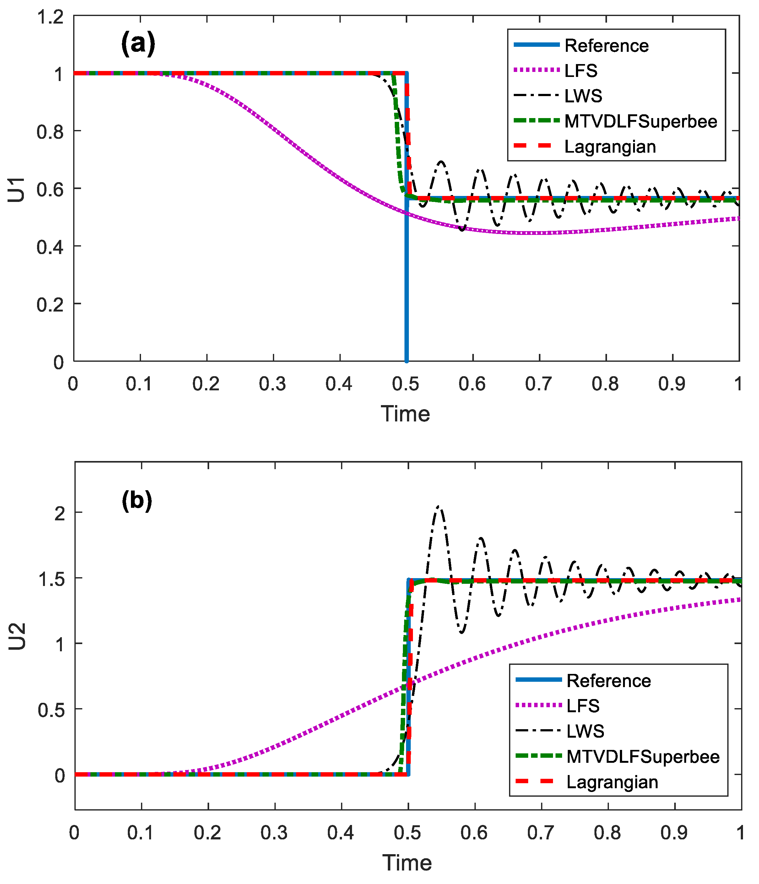
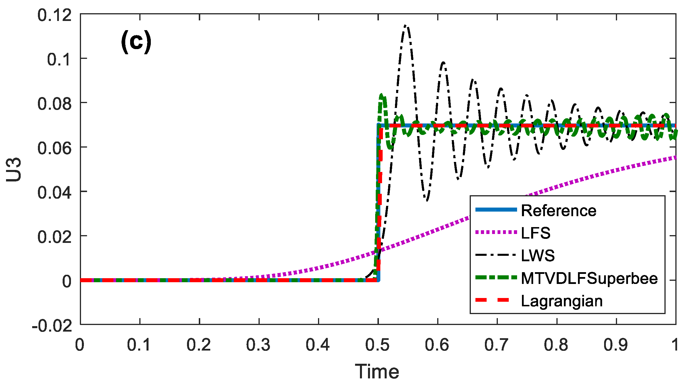
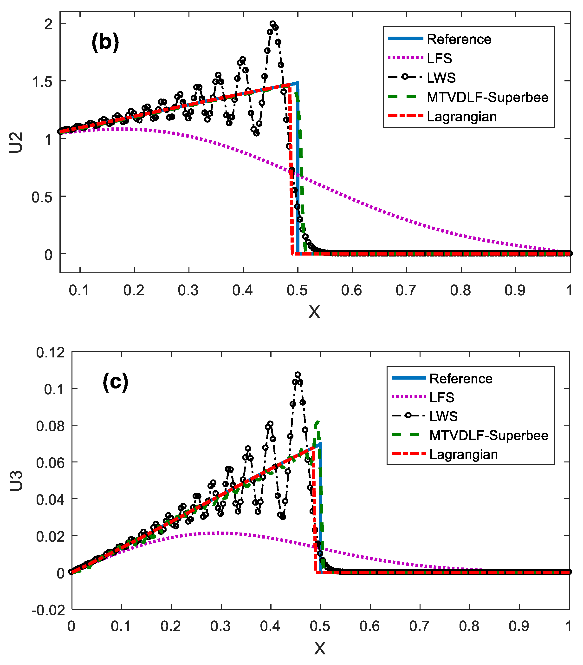
The grid number $N=200$ is employed for LFS, LWS, MTVDLF-Superbee and the proposed Lagrangian particle algorithm in the following simulations. Figure 2 compares the numerical results for the three reactants at $X=0.5$.

It is clear that UDS has good performance for both species B and C (see Figure 2b,c), but there is an evident spike close to the discontinuity for reactant A (Figure 2a), which is an unacceptable numerical defect. Therefore, even though the UDS solution can be taken as a reference, it might not be a good baseline for error analysis as conducted by Alhumaizi [7]. Reducing the grid size can reduce numerical diffusion in UDS, but it would also increase the computational time [32]. The amplitude of the spike increases with the decreasing grid size too. LFS causes serious numerical dissipation that completely pollutes the whole solution. LWS can capture the shock front but leads to unphysical oscillations behind the shock for all three reactants, due to which the numerical accuracy remarkably degenerated. The high-resolution MTVDLF-Superbee scheme is capable of yielding accurate solutions for $U_1$ and $U_2$, but it also suffers from unphysical oscillations near the discontinuity for species C as shown in Figure 2c (the solution of $U_3$ was not given in reference [7]). The present Lagrangian particle algorithm succeeded in solving the situations with steep concentration profiles without suffering from any numerical diffusion or unphysical oscillations. The results are almost the same as the reference solutions, but without any spike in the solution of species A.

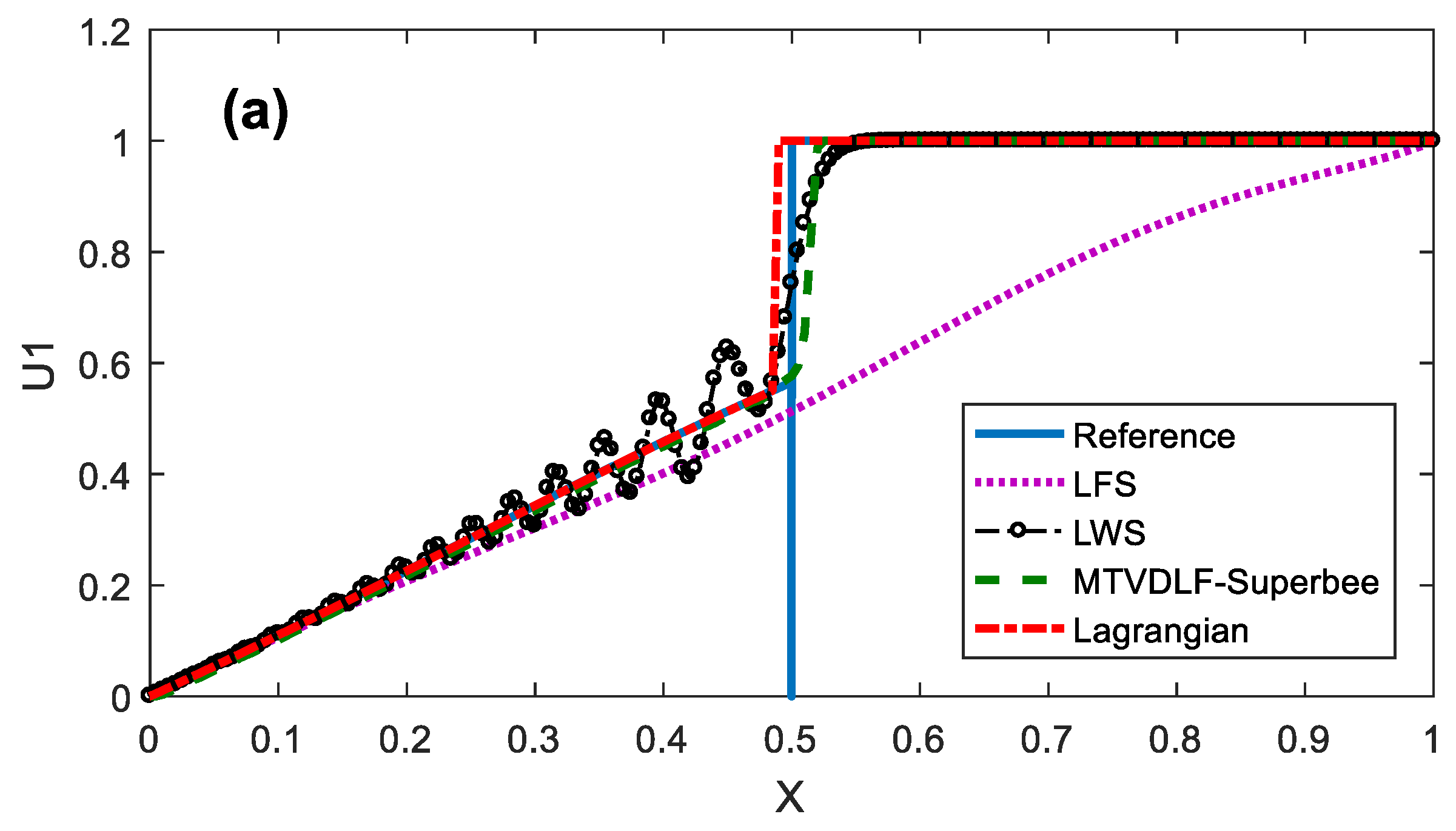
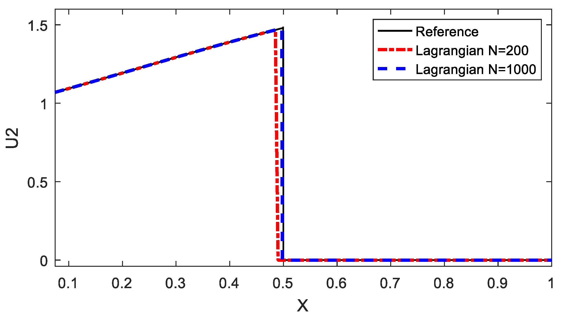
Figure 3 compares the concentration distribution obtained with different methods for the autocatalytic reaction model at $t=0.5$. Numerical dissipation and oscillations appeared in LFS, LWS and MTVDLF-Superbee are clearly shown, whilst the Lagrangian particle algorithm does not suffer from either numerical dissipation or unphysical oscillations.

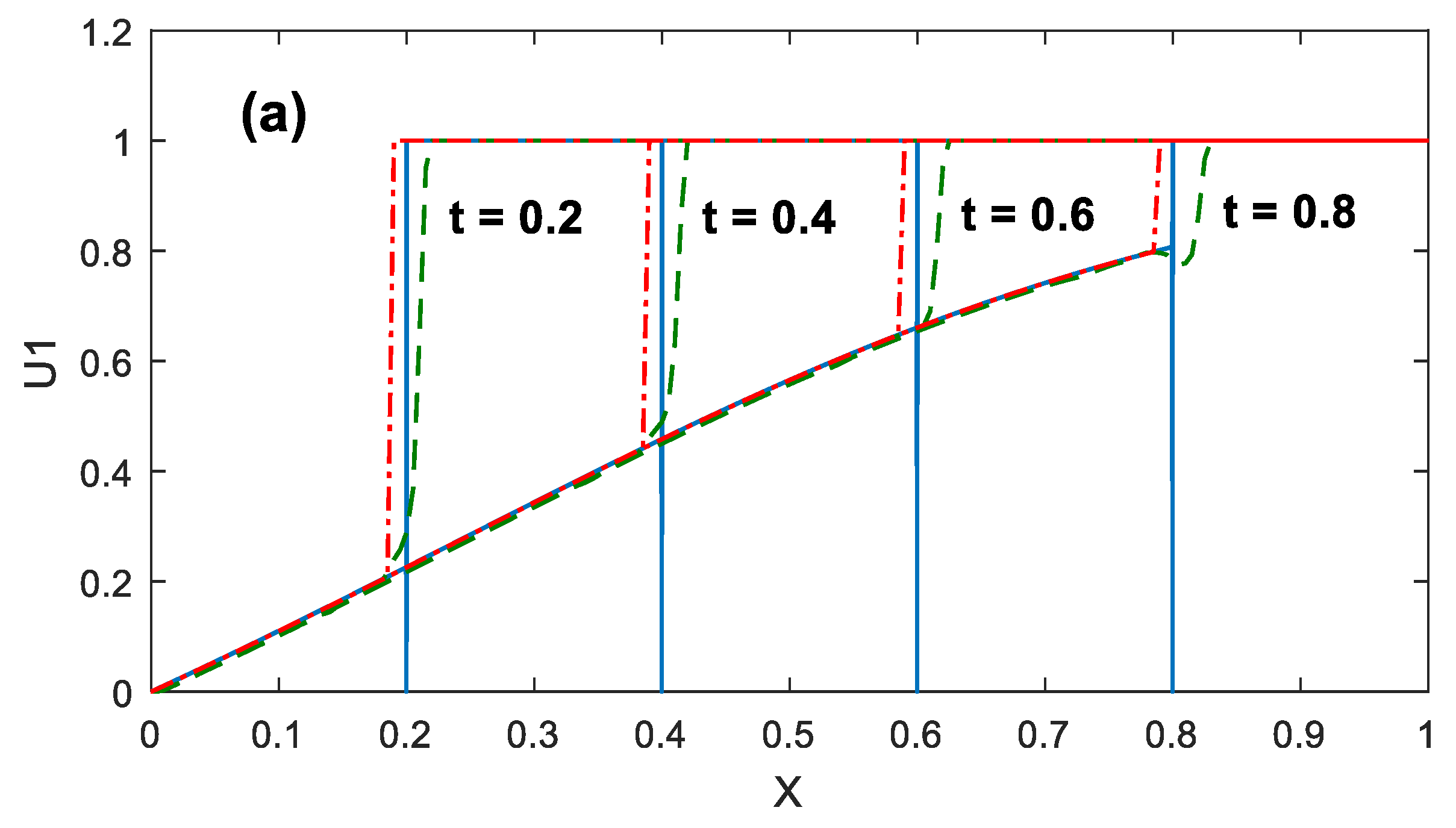
The concentration profiles obtained with different methods at four time levels are shown in Figure 4, together with the reference solutions. The results of LFS and LWS are not shown due to unacceptable numerical dissipation and spurious oscillations. It is clear that, in the reference solutions, there are the same evident spikes near the discontinuity for reactant A (see Figure 4a). Unphysical oscillations exist in the solutions of the MTVDLF-Superbee scheme for species C (see Figure 4c), and the oscillation amplitude increases with an increasing time. The Lagrangian particle algorithm has somewhat profile shifting characteristics as before, but it is capable of eliminating numerical dissipation and suppressing unphysical oscillations.

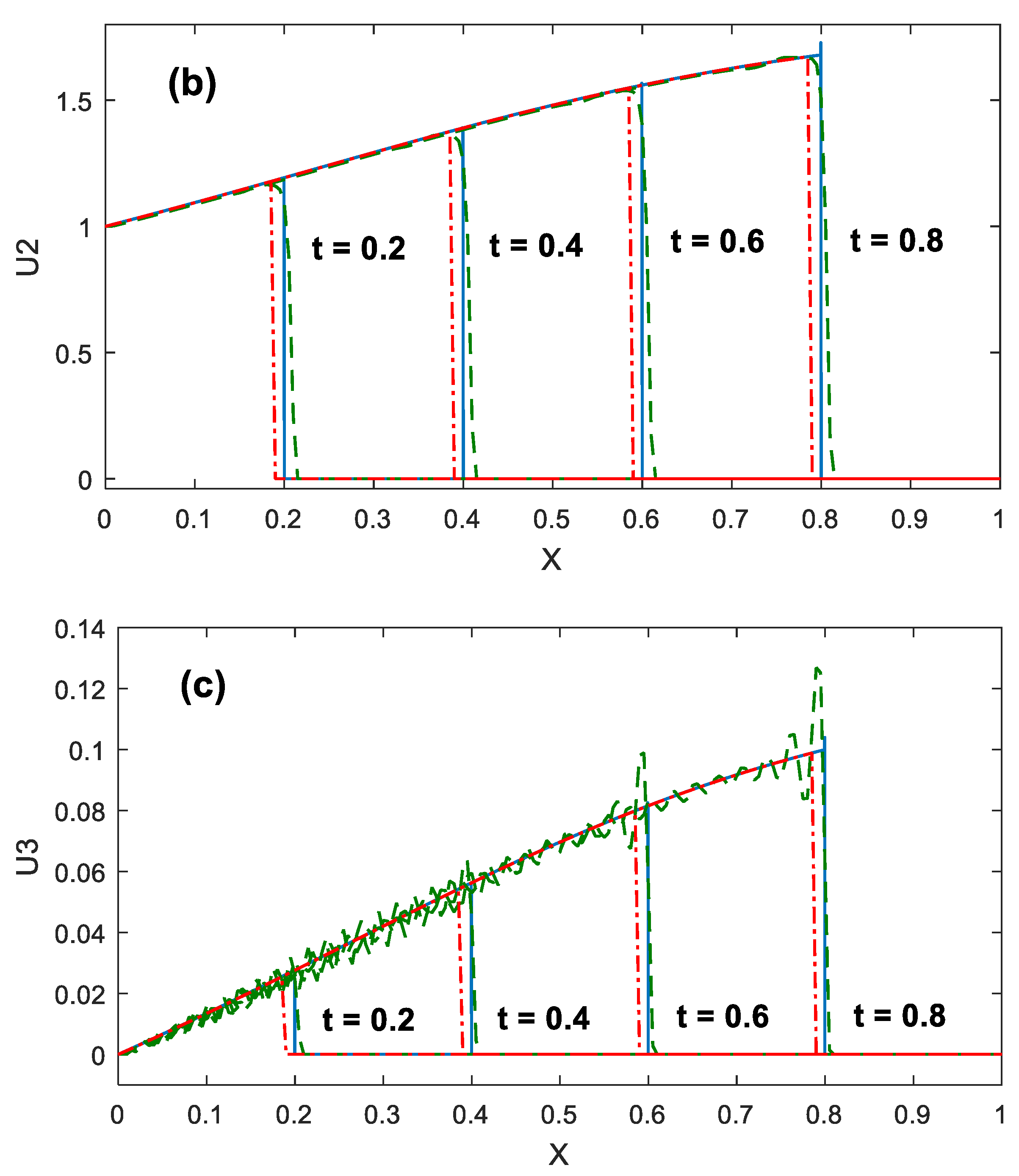
The front shifting is mainly due to a lack of particles and can be overcome by simply increasing the particle number. When particle number is increased to $N=1000$, there is no profile shifting anymore as shown in Figure 5 for the reactant concentration of species A. A similar performance holds for species B and C.

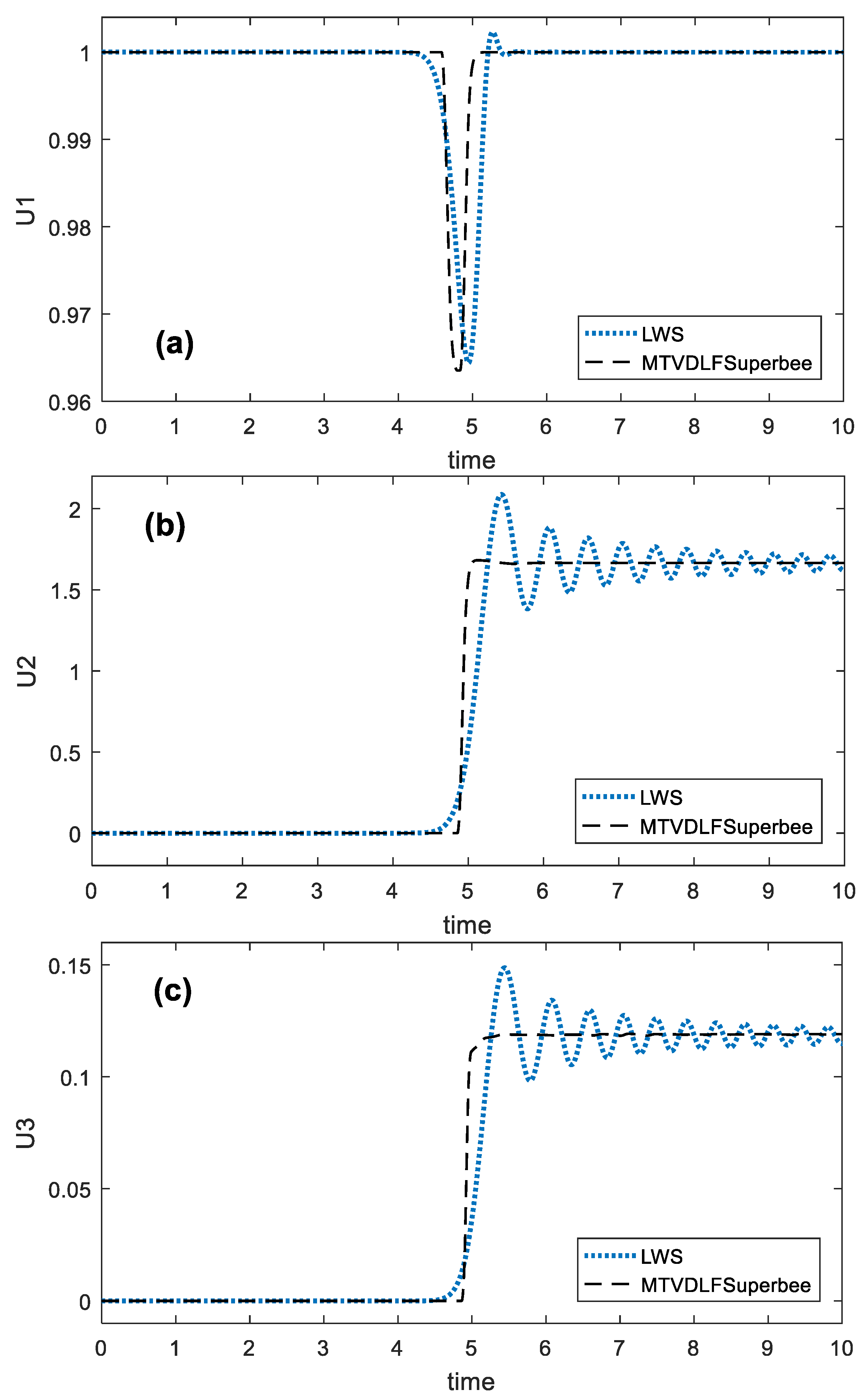
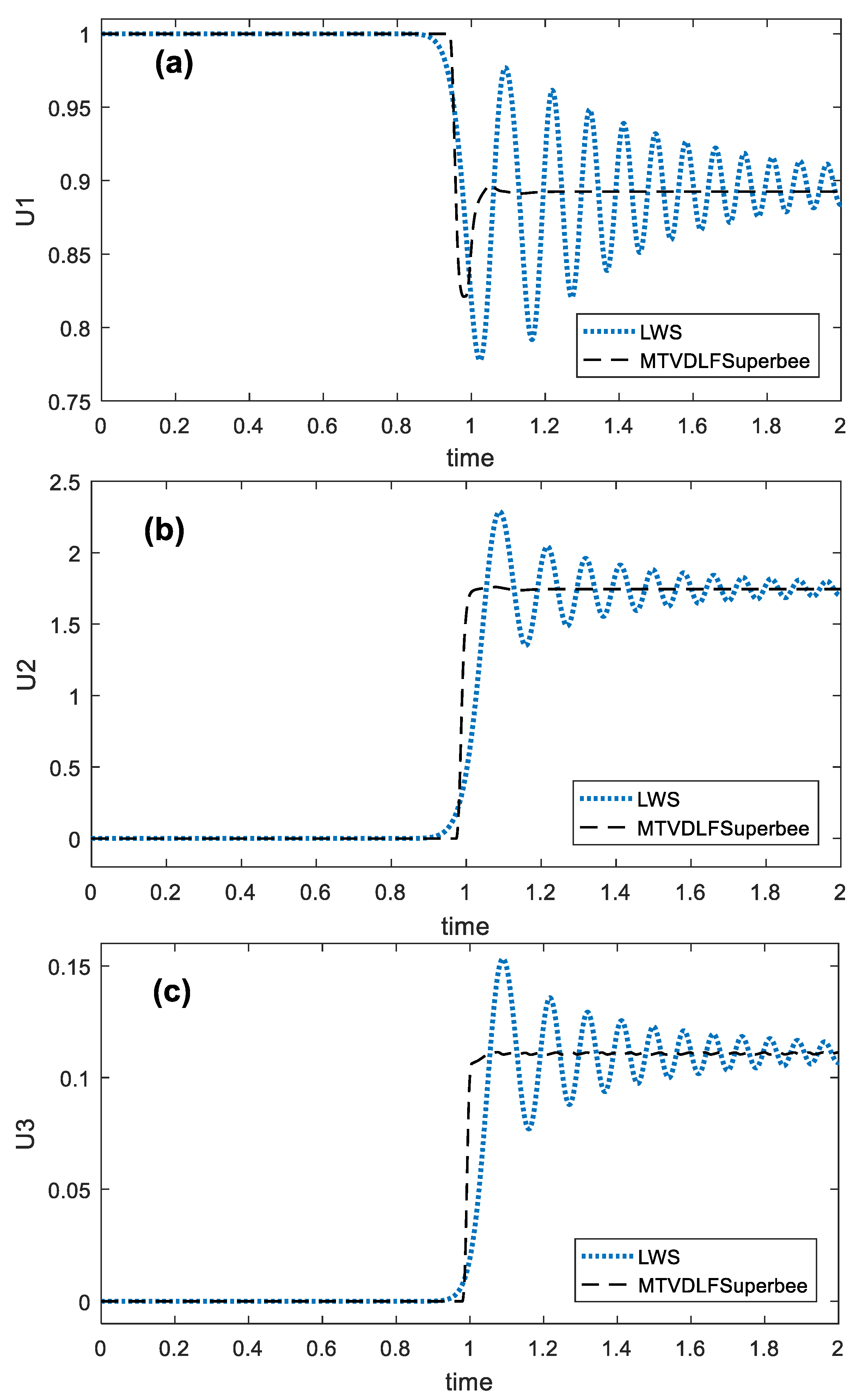
To further investigate the effects of flow velocity on numerical oscillations appeared in LWS and MTVDLF-Superbee scheme, additional experiments were conducted for cases with $V=0.1$ and $V=0.5$. The time step size and the grid number remain unchanged. The simulation times were increased to 10 and 2, respectively, to ensure the same flow distance of the fluid. The results for three reactants at $X=0.5$ are shown in Figure 6 and Figure 7, respectively. It is clear that LWS still suffers from unphysical oscillations for all three reactants in both cases with $V=0.1$ and $V=0.5$. The oscillations in the case with $V=0.5$ are relatively larger than those in the case with $V=0.1$. This is because with increasing flow velocity, the convection-reaction process is becoming more convection dominated. The MTVDLF-Superbee scheme still generates oscillations in $U_3$ (Figure 6c and Figure 7c) in all the two cases, but the amplitudes are much smaller. Slight oscillations appear in $U_1$ (Figure 7a) and $U_2$ (Figure 7b) for the case with $V=0.5$, whilst no visible oscillations appear in the case with $V=0.1$ (Figure 6a,b).

6. Summary, Conclusions and Future Research

The aim of the paper is to develop a numerical method for convection-dominated reacting flow problems without suffering from the numerical dissipation and unphysical oscillations that have existed in traditional grid-based Eulerian methods. Based on the meshless smoothed particle hydrodynamics (SPH) method, a Lagrangian particle scheme has been proposed for solving the autocatalytic reaction model with multicomponent reactants. For a better illustration of the proposed particle scheme, four typical Eulerian methods were also studied, including the first-order accurate UDS and LFS, the second-order accurate LWS and high-resolution MTVDLF with Superbee limiter.

Numerical results indicated that the MTVDLF-Superbee scheme is capable of yielding more accurate solutions than the other three Eulerian methods. This is consistent with Alhumaizi’s conclusion that the MTVDLF-Superbee scheme is the most appropriate method for simulating the autocatalytic reaction model [7]. However, MTVDLF-Superbee still suffers from unphysical oscillations near the shock region for a certain component reactant. This will greatly reduce the accuracy of the solution. However, the proposed Lagrangian particle algorithm can successfully solve the autocatalytic reaction model without any numerical diffusion and unphysical oscillations. It is therefore considered to be an effective numerical method for completing the convection-reaction models.

As the reaction flow model considered in this work is governed by the convection-reaction equations, there will be no differential operators in the governing equations after being transformed into the Lagrange system. As a result, there is no need to apply the SPH approximation for derivatives in the proposed Lagrangian particle scheme. However, when the diffusion process needs to be included, derivative approximations will be necessary. This is being worked on and will better illustrate the advantages of the proposed Lagrangian particle scheme.