1. Introduction
The application of liquid-liquid extraction (LLE) is widespread in the chemical industry. It is often applied in areas, where distillation is not feasible. Prominent examples are the separation of organic compounds from aqueous feeds, e.g., phenoles from waste water, or the separation of non-volatile components, e.g., metal ion extraction in hydrometallurgy, the recovery of caprolactam from nylon manufacturing and the wet purification of phosphoric acid [
1,
2]. However, especially in biologics manufacturing and in regulated industries in general, LLE is rarely part of the process chain, although it was shown in numerous cases to offer decisive advantages in terms of capacity, ease of scale-up, continuous operation and costs [
3,
4,
5,
6,
7,
8]. This is mainly due to a lack of knowledge regarding the practical aspects of this technology. This includes multistage operation and scale-up. Multistage operation in extraction columns is the common approach to maximize efficiency. How to perform the process development and especially the scale-up aspects of this technology are not widely known, except for supplier industry and some parts of academia, mainly institutes that conduct research in the field of process engineering with a focus on modeling. Furthermore, the current industrial practice of scaling-up extraction columns is heavily reliant on pilot-scale experiments, which are time and material consuming [
2,
9,
10]. While this alone is already a challenge to be overcome, for biologics manufacturing the more critical outcome is, that those methods are by nature empirical. Thus far, no prediction is possible due to the lack of process understanding, and therefore, no link between process and quality aspects can be made. This prevents current industrial process development practice for Quality-by-Design (QbD).
QbD-based process development is becoming the standard for new pharmaceutical products, such as virus-like-particles, plasmid DNA, fragments, etc., since it ensures quality through the whole lifecycle and allows, even demands, changes to the process after filing when optimization potentials occur, and because no comparable platform processes exist, as for monoclonal antibodies [
11,
12,
13,
14].
The application of QbD-principles for process development however requires a validated design space that guarantees constant quality, which can either be developed by experiments or by process understanding. Neither the pilot-based experimental method nor common scale-up equations are applicable for this purpose of resource efficient design space validation. Hence, there is a need for predictive LLE process models as wells as a reliable workflow that distinctively and quantitatively validates prediction precision and accuracy. Sixt et al. [
15] demonstrated the concept with an example of solid-liquid extraction (SLE). Here, we demonstrate it using an example of LLE.
The overall development workflow for a QbD-derived process is shown in
Figure 1. In the beginning, a quality target product profile (QTPP) must be derived. This is necessary to define what is critical for product quality. Characteristics for biologics are for example sterility and purity, but also certain therapeutic effects, bioactivity and dosage. Depending on the QTPP critical quality attributes (CQAs) are to be defined, which is a property or characteristic that ensures desired product quality when controlled within a defined limit, range, or distribution [
12,
16]. In accordance with the QbD-philosophy, CQAs are dynamic rather than static and have to be updated during the lifecycle of products, when newly developed product and process knowledge suggest so. CQAs guide the further process development and are derived by risk management and experimentation.
Risk assessment is part of the risk management and should be performed early in process development. Its purpose is to establish known and hypothetical links between material, equipment and process parameters and CQAs, setting the range of the further process design. Common tools for this, that are also suggested by the FDA (U.S. Food and Drug Administration), EMA (European Medicines Agency), PDA (Parenteral Drug Association) and ICH (International Council for Harmonisation of Technical Requirements for Pharmaceuticals for Human Use), are the construction of Ishikawa diagrams, also known as fishbone diagram, and the performance of a failure-mode-effect-analysis (FMEA) [
17]. Both are shown in
Figure 2. The Ishikawa diagram basically summarizes different groups of effects, e.g., properties of materials, equipment design and process parameters that can represent a risk to certain CQAs, such as yield, purity or processability in general. The major branches are fanned out into minor branches, which reveal a more detailed causality between potential cause and risk. The degree of detail is only dependent on the amount of prior knowledge that the process development team has gathered. This diagram can already reveal critical process parameters (CPPs) that must be kept within a certain range during the process, and therefore should be part of process control strategy and might be needed to be investigated in more detail.
A more quantitative tool during risk assessment is the FMEA. It is summarized in
Table 1, graphically represented in
Figure 2 and is derived by scoring the range of possible CPPs, identified in the Ishikawa diagram, regarding the possible impact that an occurring risk will have on quality attributes and the possibility that the risk will occur in the process of a stirred extraction column. It may be useful to include the chance of detecting the occurrence into the score. It is also possible to link certain parameters to each other, to also score potential interactions; however, this requires an even vaster prior knowledge about the system properties, which is seldom the case and therefore not shown here. Regarding LLE stirring intensity, in agitated columns, and the amount and presence of unwanted particles both can have a significant effect on process performance. While higher specific energy input causes an increase in hold-up, particles often hinder the coalescence of small droplets [
18]. If not controlled and kept within a certain range, both can lead to column flooding, and therefore pose a high risk to the process stability. However, while the range of energy input is efficiently controlled by operating only at certain stirring rates, the occurrence of unwanted particles can easily be missed, if turbidity measurement of the feed or robust filtration is not part of the process and control strategy. This early risk management also offers guidance for the general process development, as for this example it already highlights settling-properties as key aspects during solvent selection.
Looking back at the overall QbD-based process development strategy (
Figure 1) reveals that the next steps are focused on determining the design space. Traditionally this is done solely based on experiments. To reduce the huge experimental effort, Design-of-Experiments (DoE) methods are usually applied. Even then, the amount of raw feed material necessary in the early process development stage might already be a criterion not to choose extraction technology for high-value products or lead to an experimental design that is limited to the fewest number of experiments possible or even eliminates the possibly more efficient unit-operation altogether, since there simply is not enough material at this stage to run the necessary tests. The development of a process-analytical-technology (PAT) supported control strategy and the continual improvement are the last steps in process development strategy, but they are beyond the scope of this work. More details regarding PAT-supported control strategies and continual improvement can be found in Kornecki et al. [
19].
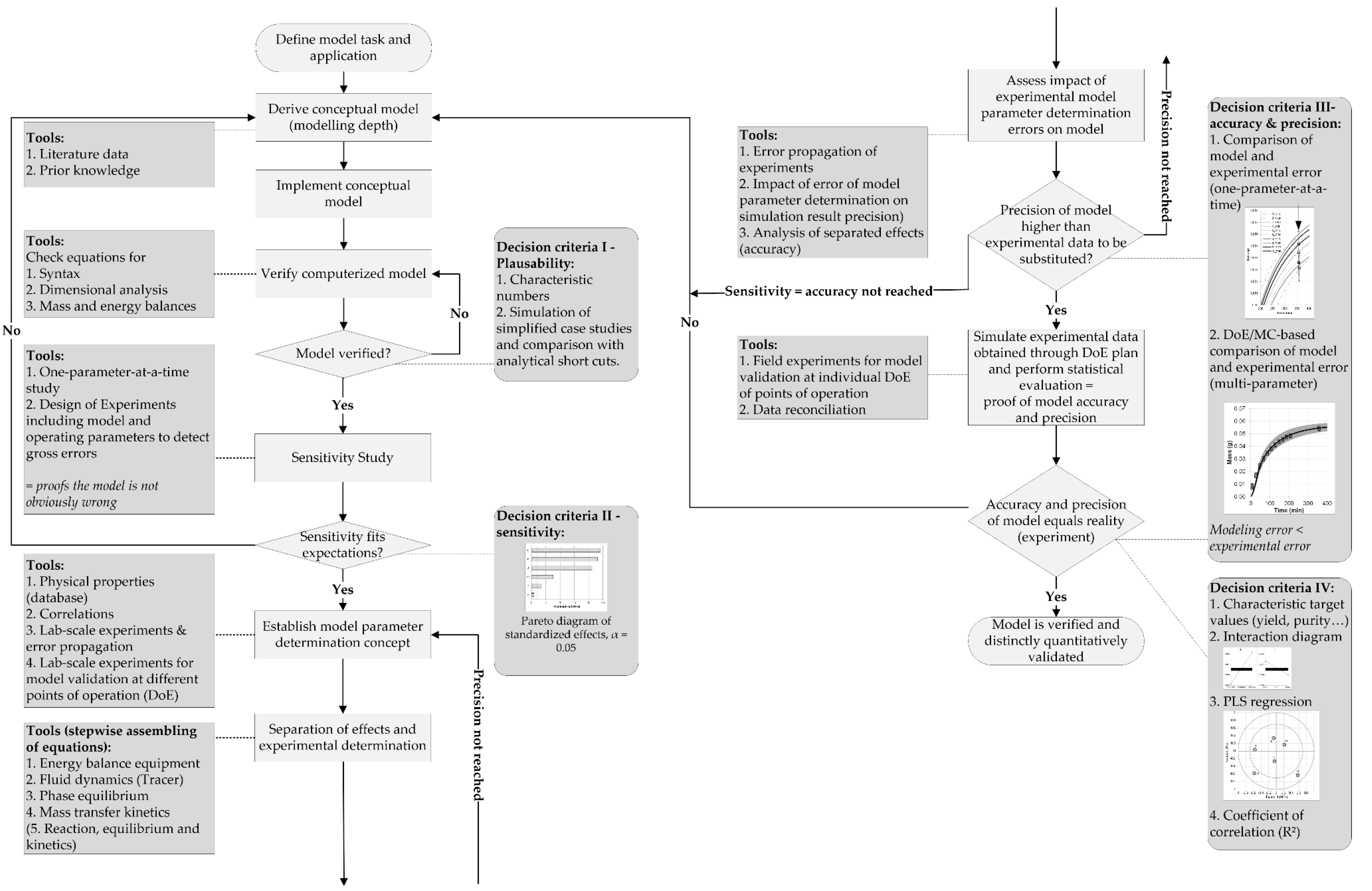
Predictive process models are the key-enabling tool to find a quantitatively defined and knowledge-based process optimum and design-space. They accelerate process development and at the same time generate process knowledge. They help to reduce the experimental effort and their validity does not end in the filed design space due to the physico-chemical nature of predictive process models. Each model that is to be utilized in this manner must be proven to be at least as accurate and precise as the respective experiments it ought to substitute. This requirement leads to the workflow for process development and validation as shown in
Figure 3. First introduced by Sixt et al. [
15], it is based on four distinct decision criteria for each development and validation phase [
14,
15].
First, the model task and its application must be defined. In case of LLE, the concentration profile in the extraction column must be correctly predicted by taking all effects (fluid dynamics, phase equilibrium and mass transfer kinetics) into account. Combining prior knowledge and studying existing literature results in the derivation of the appropriate model approach and depth. Simply, mass and energy balance checks on the example of simplified case-studies are sufficient to decide, if the conceptual model is verified.
Second, the sensitivity of the model must be investigated. Therefore, one-parameter-at-a-time studies can reveal if the model behaves in a way to be expected by an experienced process engineer. Therefore, step size of variable change should be rather large to exemplify parameter effects. However, multi-parameter-at-a-time studies are more suitable to quantify sensitivity. By applying DoE-principles a screening design can serve as plan for simulation studies. The investigated space should in contrast to one-parameter-at-a-time-studies be within the system specific boundaries, e.g., the solvent ratio in an extraction column is limited by the mutual solubility, as is the maximum loading limited by the density difference between both phases. Details on the sensitivity analysis are given in
Section 4.1.
Third, field experiments at specific points of the DoE simulation must be done, in order to compare precision and accuracy of the model at different operating points to the experiment. Last statistical evaluation such as PLS (partial-least-squares) loading plots help to quantify the results from the simulation studies.
The objective of this article is to present the complete walkthrough using an example of a monoclonal antibody and Artemisinin, both representing products from highly non-ideal complex multicomponent mixtures for regulated industries.
2. Modeling Liquid-Liquid Extraction
The use of LLE as a separation process was already known before the 19th century to produce dyes, fragrances and pigments. The basic theories of equilibrium distribution were laid by Berthelot and Jungfleisch [
20] as well as Nernst [
21]. These findings were soon followed by the first industrial applications, such as countercurrent configuration, and technical developments, such as stirred extraction columns [
22].
The methods developed for the design of processes in the first half of the 20th century still exist today in industrial practice. Major milestones before 1950 were the introduction of mass transfer coefficients by Lewis [
23], stage construction and graphical methods in equilibrium representations by McCabe and Thiele [
24], Kremser [
25] and Hunter and Nash [
26], as well as the concept of solute transfer units introduced by Colburn [
27].
In the 1950s, progress was made in identifying fluid dynamics as a major contributor to the effects that are crucial in predicting LLE in technical applications. The fact that there is a large deviation from plug-flow regime in extraction columns, and therefore a diminished efficiency, was made by Geankoplis and Hixson [
28], Burger and Swift, Sege and Woodfield [
29] and Thornton and Logsdail [
30]. Danckwerts [
31] introduced theaxial dispersion model (ADM) as a mathematical description of plug-flow overlapped by backmixing. Alongside with other researchers Levenspiel and Smith [
32], Sleicher [
33] and Stemerding and Zuiderweg [
34] were on the forefront in contributing to this model concept, developing methods to determine the dispersion coefficient and to quantify the effect of axial dispersion on separation efficiency.
In the 1960s, Miyauchi and Vermeulen [
35] were among the first to apply the DPF model and calculate concentration profiles in extraction columns. Additionally, limitations of this model approach were discussed, among others by Rod [
36], who introduced the term “forward-mixing”, partially caused by so-called channeling.
From the 1970s to the 1980s, many working groups discussed if deviation from plug flow, caused by different convective velocities of drop size distributions, can be represented by the axial dispersion model. A summary of available model approaches developed during this period was done by Steiner and Hartland [
37]. While some researchers found good agreement with axial dispersion model predictions and experimental data like Reissinger [
38], the development of models that specifically account for coalescence and breakage of drops by population balance models (PBM) began. Jirnicy et al. [
39,
40], Cassamata and Vogelpohl [
41], Haverland et al. [
42], Al Khani et al. [
43], Cruz-Pinto and Korchinsky [
44], Coulaloglou and Tavlarides [
45], Tavlaritis and Bapat [
46] and Hamilton and Pratt [
47] were the major contributors to develop and expand on this model type. The three major modeling approaches to LLE in extraction columns at this point in time and their respective system boundaries are shown in
Figure 4.
In the 1990s, computational capacities increased significantly, and thus, many research groups focused their research development on PBM and more sophisticated kernels to calculate coalescence and breakage in more detail. Major contributions were made by the research groups of Bart and Pfennig, for example in the work of Kronberger et al. [
48] and Henschke et al. [
49].
More recently, research began to focus on the fact that the increase in model depth had to be supplemented by parameter determination concepts in order to be predictive. Among others, Hoting [
50] published model prediction for the EFCE (European Federation of Chemical Engineering) standard test system water, butyl acetate, acetone in packed extraction columns. The project “from single-drop to extraction column” focused on PBM approaches and could show for packed and agitated columns scale-up was possible on the example of the EFCE standard test systems [
51,
52,
53].
Franke et al. [
54], Leistner [
55], Eggersglüß [
5,
6,
7] and Wellsandt [
56] from the research group of Strube worked on parameter determination concepts for complex feed mixtures and demonstrated the feasibility of model based process development Since then, some research dives even deeper into modeling depths by combining CFD with PBM [
57]. However, for industrial use and the prediction of processes including complex feed mixtures, the axial dispersion model still is the approach of choice, due to accounting for all relevant effects and also the availability of more precise and efficient model parameter determination concepts.
Axial Dispersion Model
The fundamental equations of the axial dispersion-model are based on the transport equations for the continuous (see Equation (1)) and the dispersed phase (see Equation (2)). They describe the mass balance around the system boundary as shown in
Figure 4 (middle). The accumulation term on the left hand side of the equations is the sum of the change in concentration due to the convective mass flow, mainly characterized by the velocity
, the dispersed mass flow, mainly characterized by
, and the mass transfer between both liquid phases depend on the effective mass transfer coefficient
, hold-up, sauter diameter
and equilibrium concentration
:
In the extraction columns, there is a deviation from the ideal plug flow due to back-mixing. This leads to a deviation from the ideal residence time distribution and thus to different contact times between the dispersed and the continuous phase. The result is a decreased separation efficiency [
6,
7]. This so-called dispersion can be characterized by the axial dispersion coefficient
, which is either experimentally determined for the continuous and the dispersed phase by tracer tests or by corresponding empirical correlations. Depending on the column type and internals different correlations are published. For the continuous phase, the approach in Equation (3) is often applied:
In addition to the stirrer diameter (
DR) and the stirrer speed (
N), the Equation also contains the constants (
C1,
C2 and
C3), which account for different geometries of stirrer and column. Therefore, the coefficients are selected according to the column type, its diameter and overall stirrer geometry [
58,
59,
60,
61]. A modified correlation from Rod and Misek for the axial dispersion coefficient of the dispersed phase for Kühni columns can be seen in Equation (4) [
62]. As for the continuous phase, there are several correlations published that are determined for specific column scales and geometry [
63,
64,
65].
The cross-sectional column loading (
L) is another important parameter for the characterization of column efficiency. It is defined as the sum of the volume flows of the continuous (
VC) and the disperse phase (
VD) divided by the column cross-sectional area (
AC):
The corresponding differential equations can be solved by the implementation of two boundary conditions for the continuous and dispersed phase, which are shown in Equations (6) and (7):
3. Model-Parameter Determination
For the application of the axial dispersion model in process design, the determination of a set of model parameters is necessary as described in the section before. Ideally, the complete set of parameters can be determined with as few experiments as possible and thus with as little material and time as possible. However, this requires a standardized and effect oriented model parameter determination concept. The workflow to determine model parameters, which are needed for the DPF-model, is shown schematically in
Figure 5.
The sequence to determine these parameters are ordered according to their importance and effect on the process:
1. Fluid dynamics (red): the fluid dynamic behavior of the system is dependent on the axial dispersion of the system, as well as on the hold-up (
Figure 5, 1.1), characterized by drop rise velocity, droplet sauter diameter and column loading. The axial dispersion coefficient must be determined by tracer experiments (
Figure 5, 1.2) if it is not to be determined by correlations. Since this parameter is primarily geometry-dependent, the actual feed solution does not have to be used. Around 2–5 L of total system volume, depending on the investigated scale, is required for the determination of axial dispersion behavior. A qualified person can perform this experiment within 1 day.
A droplet measurement cell can be used for the quantification of the drop size and drop rise velocity (
Figure 5, 1.3), which is dependent on the sauter diameter. Few milliliters, up to 50 mL, are required to determine this parameter within 1 to 5 days. Batch-settling experiments to determine the settling time and properties of the system can add additional information regarding which solvent to choose for the process (
Figure 5, 1.4); however, they are not mandatory for the parameter determination.
2. Phase equilibrium (blue): shaking flask experiments must be performed to determine the binodale, tie-lines and distribution coefficients of target and main side components. Up to five points evenly spread around the phase diagram can typically deliver the necessary information. Between 5 and 10 mL are usually enough per shaking flask experiment to determine these parameters. However, if interfacial tension, viscosities and densities for both phases are not known or accessible by reliable database or correlation, the volume should be increased to obtain these data also from the shaking flask experiments. If determined in triplicates, 75 (3 × 5 × 5 mL) up to 150 (3 × 5 × 10 mL) mL of system volume are needed for the quantification. Up to 2 days are sufficient for execution.
3. Kinectics (green): the effective mass transfer coefficient is necessary to correctly describe the kinetic of the extraction process. Lower values of this parameter result in more time necessary for component separation. This parameter can also be quantified by droplet measurements, and thus, should be determined parallel to the drop measurements during the 1 to 2 days period.
The time and material resources necessary for a complete model parameter determination as described above requires around 3 days up to 1 week and only 200 up 300 mL feed material. More detail for each model parameter experiment can be found in [
66].
4. Model Validation
In the following subsections, we show the decisive steps during the model validation. First, syntax, mass and energy balance must be checked. It is advisable to also test if the principle model behavior is logical, e.g., that mass transfer direction is correct. Exemplary case studies, either from in-house data or from literature can help to identify a suitable reference point and to show that the model is not obviously wrong.
4.1. Sensitivity Analysis
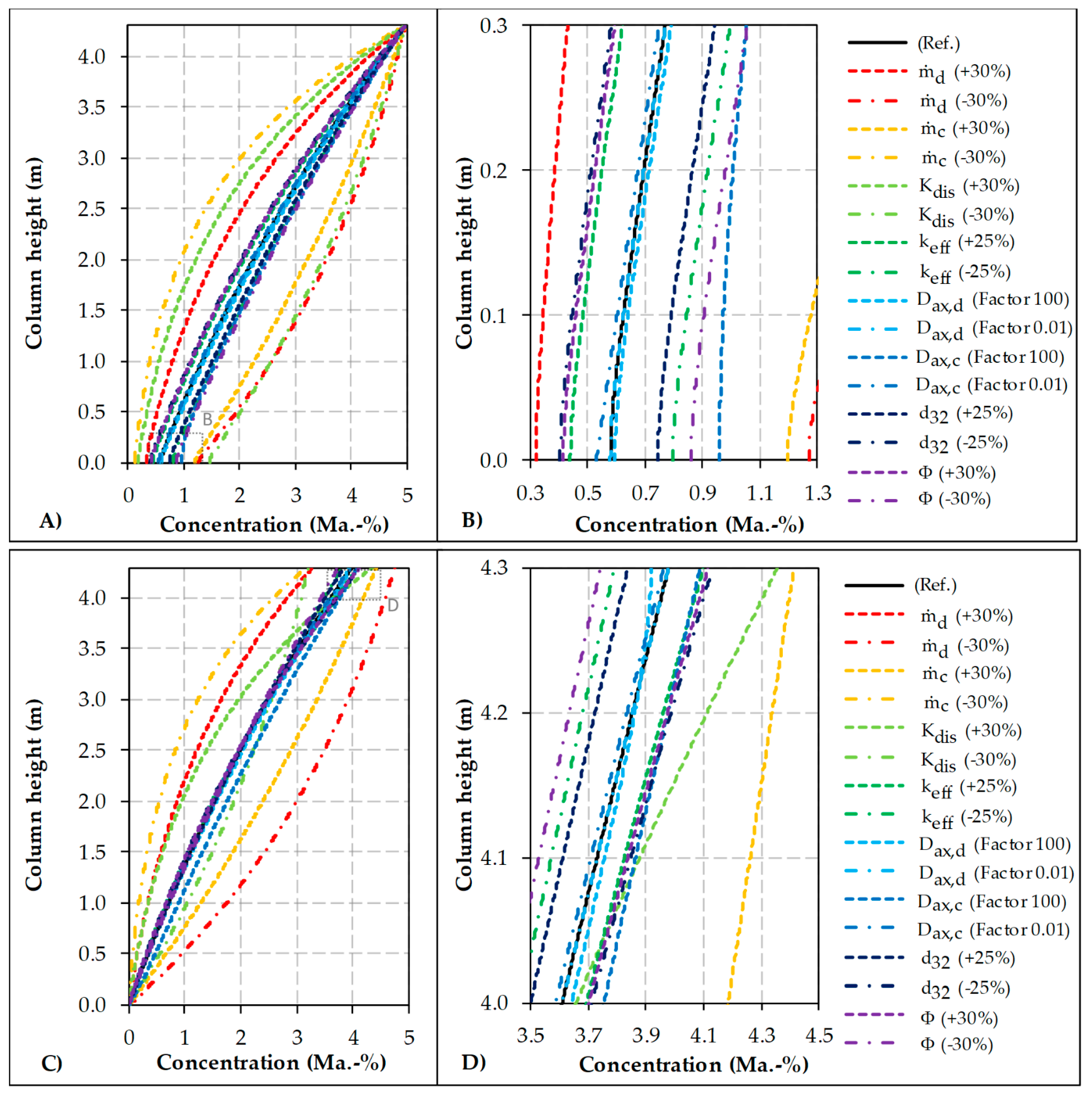
As described in the introduction, the next steps are one-parameter-at-a-time sensitivity studies. Here, data from Hoting [
67] were used as point of reference. The parameters for the sensitivity analysis are shown in
Table 2. It was investigated how big the influence of each parameter is, when the others are kept at their default value.
Figure 6 shows the result for the first sensitivity study. The mass flow of the dispersed and continuous phase affects the concentration profile the most. This is to be expected, as they determine the solvent ratio and whether the feed stream is depleted from the solute by the solvent stream or whether the solute quickly reaches equilibrium concentration in the solvent stream. The distribution coefficient has a default value of approximately 1. Thus, a variation of this parameter of 30% is enough to induce a change of the concentration profile similar to the effects of the solvent ratio. The other parameters, such as hold-up, sauter diameter and axial dispersion, only show small influences on the concentration profile when kept within reasonable values (see
Table 2).
The next step during sensitivity analysis is the performance of multi-parameter-at-a-time studies. This reveals parameter combinations that have a significant effect on a CPP such as purity or concentration. Therefore, it is recommendable to apply a DoE-derived simulation plan, which mimics the experiments plan otherwise necessary for optimal operation space identification. This will be shown in the following using as an example the purification of Artemisinin.
Table 3 summarizes the Plackett-Burman-Design for the simulation studies, which is typically used in the early process development stage to screen for the most important factors that influence the process outcome [
68]. The combined mass flow of the continuous and dispersed phase are limited by the flooding point of the system, which was determined to be around 12 m
3/m
2/h, the minimum solvent ratio. The concentration of Artemisinin and the side components are variable due to the natural raw feed material variability. The other parameters are set within the range of what can occur during the process.
Figure 7 shows the Pareto chart of standardized effects obtained from the simulation runs. The statistical criterion of significance here is the p-value. If the model parameters are evaluated by the increase in Artemisinin concentration; then, it becomes clear that the massflow of the continuous and dispersed phase are the most significant factors. Since the distribution coefficient of Artemisinin is comparably high, mass transfer is fast and equilibrium composition is reached very quickly. Larger deviations of other parameters that influence mass transfer, such as the effective mass transfer coefficient, sauter diameter and hold-up become therefore non-significant. Thus, the concentration of Artemisinin is mostly determined by the solvent ratio. The third significant parameter is the distribution coefficient of acetone. This is also easy to understand, since acetone is also a solute that is extracted, however in much larger quantities. The more acetone is extracted, the larger the extract volume gets and the more diluted the Artemisinin concentration becomes.
4.2. Statistical Evaluation
The last steps in the model validation workflow presented here include the statistical evaluation of different operating points of the previously simulated DoE. First, the center point of the statistical simulation plan is established; second, selected optimized operating point is evaluated with regard to precision and accuracy. Finally, the simulation of an aqueous two-phase extraction in a packed extraction column serves to present the robustness of the model, which explicitly includes the secondary component profile.
Figure 8 shows the results of the center point simulation (left) and the simulation of the optimized operating point (right) compared to the experiment. Data represent experimental duplicates as well as the standard deviation. Since all model parameter determinations are subject to statistical and methodological error, these must be taken into account in the simulation to enable a reliable comparison to the experiments. This is achieved by the random, evenly distributed variation of the model parameter values in a Monte-Carlo simulation. The default values are the results obtained from the model parameter determination. The range of deviation is determined from the error calculation for each model parameter. The default values and the range of deviation for the simulation are summarized in
Table 4 and
Table 5. All process information in detail can be found in our previously published work [
69].
Both operating points are characterized by a high utilization of the column in the upper area. This fits with the previously discussed findings that the distribution coefficient of Artemisinin is so large that it is fully extracted at a very early stage in the process. Therefore, the resulting concentration value at the head is only significantly dependent on the set solvent ratio, which is specified as a process parameter and can thus be optimized, and the distribution coefficient of acetone underlying the system, which determines the volume of the extract phase. An example with a more evenly spread column profile is presented later.
The simplex (enveloped curves) represents the minimum and maximum values of 100 Monte-Carlo simulation runs. As can be seen the derived model precision is within the experimental deviations. If the accuracy of the model is compared to the experiments, the center point concentration can be very well predicted (left diagram (A) in
Figure 8). The optimized operating point is derived from our previous work, that showed that the concentration can be increased by decreasing dispersed solvent mass flow towards the minimum solvent ratio, which is around 1/6 [
69]. Herein, the increased concentration (experiment and simulation) can be easily observed, which underlines the correct parameter implementation. Furthermore, a larger deviation of the simulated and experimental head-concentration can be observed in the column height of 3.5 to 4.5 m. The model inherently closes the mass balance, which is due to error in analytics, experimental procedure and product instability not necessarily reflected in the experiment. The simplex is within the experimental deviation, and therefore the necessary model accuracy is given.
Since for the model purpose of replacing experiments specified in the introduction a sufficient precision and accuracy are given, model parameter influence can now be statistically evaluated.
Figure 9 shows the partial-least-squares regression loading plot. The inner circle includes all model parameters (predictors, blue) that explain up to 50% of the observed variance. The area between the inner and outer circle contains the predictors that explain the remaining variance. Model parameters that are positively correlated to the here evaluated target component concentration (response, red) are located in the same direction of the diagram. For example, the mass flow of the continuous phase is positively correlated to the response, since its increase practically leads to more of the target component that can be extracted and indirectly decreases the solvent ratio. This is even better illustrated by the mass flow of the dispersed phase, which is located in the opposite direction of the target component concentration and therefore implies a negative correlation to the model response. This fits very well with all the above mentioned findings (sensitivity studies, Pareto-chart, comparison of experiment and simulation of two operating points, which origin from the DoE and theoretical understanding) and is the final step in the model validation workflow.
It should be noted that for other systems both the Pareto and the PLS loading diagrams will be different. For example, for a mass transport-limited system the solvent ratio is expected to be far less significant. On the other hand, the smaller the distribution coefficient of the target component in the system becomes, the more significant its influence on the concentration profile is and it should be positively correlated to the extract concentration. The same rationale is applicable for the mass transfer coefficient. However, the procedures and methods of evaluation should always be based on the procedure and the evaluation criteria shown here in order to enable an evaluation of the validity of the model for use in a QbD-based process development as discussed in the introduction and depicted in
Figure 1.
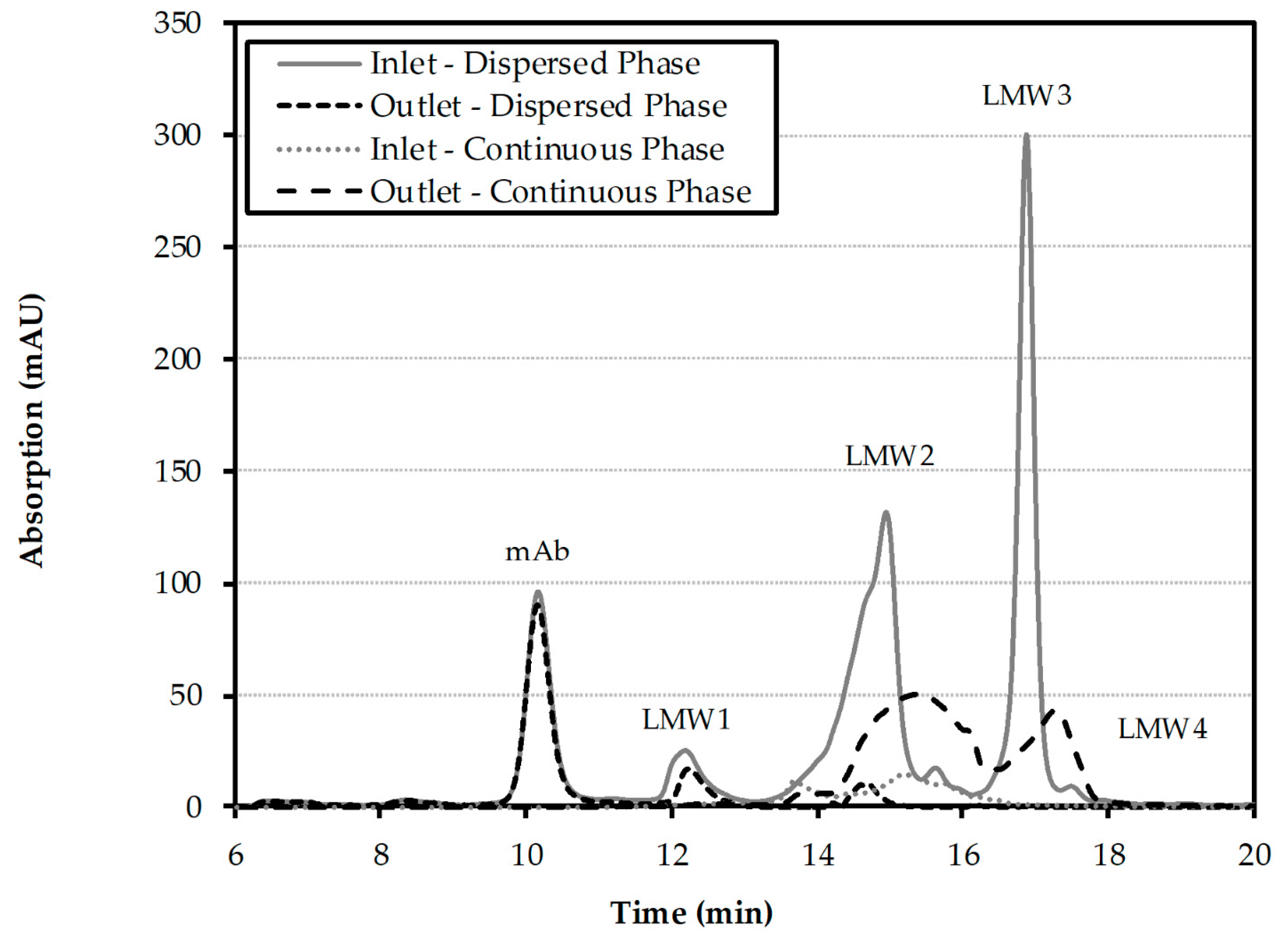
Finally, to further demonstrate the validity of the model, it is applied to the wash extraction of a monoclonal antibody (mAb). Details on the latter study are published by Eggersgluess et al. [
7] and process parameters are summarized in
Table 6. After capture of the antibody from a cell culture harvest by aqueous two-phase extraction, the mAb containing light phase is washed in multistage-operation with fresh heavy phase. The process is executed in a packed extraction column. The light phase enters the column dispersed at the bottom; the heavy wash phase enters the column as continuous phase at the top. For the design of the total process it is especially important to have information about the purity profile to be able to design the subsequent purification steps adequately. The size exclusion chromatogram of the inlet and outlet streams is shown in
Figure 10. The monoclonal antibody (mAb) peak is located at around 10 min. The following peaks can be contributed towards lower molecular weight (LMW1, LMW2, LMW3, LMW4) components, which will serve in the following as the investigated impurities. The comparison between the experimental and simulated purity profiles is shown in
Figure 11. The simulated purity profile for LMW1 and LMW4 are well within the experimental deviation. This is to be expected, since LMW1 does not show a high solubility in the continuous phase and LMW4 already is highly depleted at the column inlet. The more difficult impurities LMW2 and LMW3 are also within the experimental deviation at the column top, with larger deviations for LMW2 at the column middle. However, the critical overall purity profile is then again within the experimental deviations over the entire column length.
5. Material and Methods
The materials and methods for the Artemisinin study can be found in detail in our previously published article [
69]. Butyl acetate for the column tests was purchased from ThermoFisher (Waltham, MA, USA) in technical grade purity of 99% (by GC). Acetone was purchased from VWR (Darmstadt, Germany). The analysis of artemisinin by HPLC is performed on an Elite LaChrom
® device equipped with an Evaporation Light Scatting Detector (ELSD) Alltech
® 3300 (Grace
®, Columbia, SC, USA). The analytical column is a PharmPrep
® RP18 250 mm × 4 mm i.d. (inner diameter) by Merck
® (Merck KGaA, Darmstadt, Germany) operated at 25 °C.
The materials and methods for the mAb study can be found in detail in the work published by Eggersgluess et al. [
7]. Polyethylene glycol with an average molecular weight of 400 Da (PEG 400) and NaH
2PO
4 were obtained from Merck (Darmstadt, Germany). K
2HPO
4 and Tween-20 were from Sigma Aldrich (St. Louis, MO, USA). A cell culture harvest from a Chines hamster ovary (CHO) cell culture (harvest/cell culture harvest) was provided by Boehringer Ingelheim Pharma (Biberach, Germany). The cell culture harvest contained an IgG mAb. Size exclusion chromatography (SEC; TSKgel G3000 SWXL column; Tosoh Biosciences, Stuttgart, Germany) was performed to obtain the purity profile.
The purity
P is defined in all experiments as the area of the target component peak in the ELSD chromatogram (for artemisinin) or in the size exclusion chromatogram (for the monoclonal antibody) divided by the total area of the target component and respective side components:
The solvent ratio in all column experiments is defined as follows:
The column experiments are carried out in two mini-plant columns; a stirred Kühni column (Artemisinin study) and a pulsed, packed column (mAb study). Both columns have a total volume of approximately 5 L with an effective separation height of 3.5 m. The diameter of the separating area is 26 mm. This results in an effective separation volume of about 2 L, slightly reduced by 8 vol% by the installations.


