Prediction of CO₂ Solubility in Ionic Liquids Based on Multi-Model Fusion Method

Abstract

Reducing the emissions of greenhouse gas is a worldwide problem that needs to be solved urgently for sustainable development in the future. The solubility of CO₂ in ionic liquids is one of the important basic data for capturing CO₂. Considering the disadvantages of experimental measurements, e.g., time-consuming and expensive, the complex parameters of mechanism modeling and the poor stability of single data-driven modeling, a multi-model fusion modeling method is proposed in order to predict the solubility of CO₂ in ionic liquids. The multiple sub-models are built by the training set. The sub-models with better performance are selected through the validation set. Then, linear fusion models are established by minimizing the sum of squares of the error and information entropy method respectively. Finally, the performance of the fusion model is verified by the test set. The results showed that the prediction effect of the linear fusion models is better than that of the other three optimal sub-models. The prediction effect of the linear fusion model based on information entropy method is better than that of the least square error method. Through the research work, an effective and feasible modeling method is provided for accurately predicting the solubility of CO₂ in ionic liquids. It can provide important basic conditions for evaluating and screening higher selective ionic liquids.

1. Introduction

Nowadays, energy crises and environmental issues are frontier problems that arouse great concern. Reducing the emissions of CO₂ is one of the crucial challenges for sustainable development in the future. Carbon Capture and Storage (CCS) is by far a mature theory to study the reduction of CO₂ emissions. The ionic liquids (ILs) have some properties of low volatility, high solubility and high selectivity, which make them increasingly interesting in capturing CO₂. These advantages make the ILs considered as a relatively novel type of solvents [1,2,3,4].

The value about the solubility of CO₂ in ILs is important information. It can not only help us to study the interaction between CO₂ and ILs, but also provides important guidance for ILs design that meets industrial needs [5,6]. At present, the main methods for obtaining solubility of CO₂ in ILs include experimental measurement and modeling. Due to the difficulties, e.g., the non-ideal behavior of the research system, the complexity of ionic liquid system, the limited measurement conditions, the time-consuming and high costs on the measurement of ILs, it is impossible to obtain the solubility by the experimental measurement method for practical applications [7,8]. The modeling methods mainly consist of mechanism modeling and data-driven modeling.

The thermodynamic models have the advantages of clear engineering background, strong interpretability and good extrapolation ability. For these reasons, researchers have tried to present thermodynamic models to predict solubility of CO₂ in ILs. It commonly includes state equation, activity coefficient group contribution models, and quantum stoichiometry models.

Jaubert [9] and Lei [10] established the prediction model to determine solubility of CO₂ in ILs by Peng Robinson (PR) state equation. Soave [11] developed a model based on the Soave Redlich Kwong (SRK) state equation to predict the behavior of equilibrium constants of CO₂. Peters [12] utilized the group contribution method to prognosticate the phase behavior of binary systems of ILs and CO₂. The UNIQUAC model has been used by Coutinho [13] to calculate the activity coefficient and been applied with the PR state equation and Wong–Sandler mixing rule to correlate the experimental data of CO₂ solubility in ILs. Cornelius [14] evaluated solubility of CO₂ in ILs by using a model combined with quantum chemical calculation and a thermodynamics method.

Although the mechanism modeling methods can predict the solubility of CO₂ in ILs theoretically and accurately, they need to be supported by the mechanism knowledge of the real situations. The physical meaning of the system parameters of such mechanism modeling methods is relatively uncertain, and the calculation is complicated. The above two reasons lead to low prediction accuracy and poor model robustness [15].

Due to the high interpolation and strong learning ability of the data-driven modeling methods without any assumptions between inputs and outputs, they have been widely used to predict the solubility of various gases in different solvents [16,17].

Mohammad [16] used decision tree learning in modelling to predict the solubility of CO₂ in ILs, and the outputs of the model were in excellent agreement with the corresponding experimental values. Eslamimanesh [17] utilized the artificial neural network (ANN) algorithm to predict the solubility of CO₂ in 24 commonly used ILs, which were successfully applied for the prediction. Farmani [18] compared the ability of the ANN model and the EOS model to predict solid solubility in supercritical CO₂, and the results indicated the ANN model was able to more consistent with the experimental data. Lashkarbolooki [19] developed the ANN to predict phase equilibrium behavior in binary systems that contain CO₂, and the prediction accuracy of the model was high. Afshin [20] introduced the CMIS method to fuse all kinds of sub-models, and the obtained prediction results of CO₂ solubility in various ILs was in good agreement with the experimental values.

At present, most of the data-driven models which were established to predict the solubility of CO₂ in ILs are single models. However, these models are prone to the local optimization and cannot describe the global characteristics of the problem. Therefore, the prediction performance of these models is limited.

In order to overcome the shortcomings of mechanism modeling and data-driven modeling in predicting the solubility of CO₂ in ILs, a multi-model fusion modeling method combing the Back Propagation (BP), Support Vector Machine (SVM) and Extreme Learning Machine (ELM) sub-models is proposed. After applying proposed models to predict the solubility of CO₂ in ILs the effectiveness of multi-model fusion models will be verified.

2. Methods

2.1. Single Modeling Method

2.1.1. Back Propagation Neural Networks

Back Propagation Neural Networks (BPNN) is a supervised learning method that simulates the perception of the world by biological neurons. The training process consists of forward propagation of signals and back propagation of errors. The input signal begins to diffuse from the input layer to the hidden layer and is output by the output layer after a series of processing [21]. If the result of forward propagation yields the expected output, the learning process will be terminated. Otherwise, the weights and biases between different neurons will be adjusted layer by layer according to the gradient descent method till the expected minimum of the target function is reached. The BP neural network has high nonlinear mapping ability and flexible network structure. It has been widely applied in many fields of chemistry, chemical industry and economy that have a degree of difficulty and are complex to solve.

The approximation and generalization ability of the BP neural network model strongly depends on the samples [22,23]. The convergence velocity of the algorithm of the model is slow, and is easily trapped to a local optimum. In the process of establishing the BP neural network model, the undertraining and overtraining of model will affect the prediction effectiveness. Therefore, it is important to reasonably select the number of the hidden layers and neurons in each hidden layer [24].

2.1.2. Support Vector Machine

Support Vector Machine (SVM) is a supervised learning method that is developed from statistical learning theory and is similar to neural network [25]. The basic idea of this design is based on Vapnik Chervonenkis (VC) dimension theory and structural risk minimization principle. Under the finite sample information, the complexity and learning ability of the model are adjusted by constructing the loss function, and then the model with better prediction performance is established.

In the process of developing a support vector machine model, different kernel functions and non-linear mapping can map the input patterns into different higher dimensional linear feature space [26,27]. In order to obtain better performance of SVM models, it is necessary to select the kernel function type and optimize the relevant parameters of the kernel function reasonably. The commonly used kernel functions are polynomial kernel function, radial basis kernel function and sigmoid kernel function.

The expression of the polynomial kernel function is as follows:

$$K\left(x_i,x_j\right)={\left[\left(x_i\cdot x_j\right)+1\right]}^q.$$

(1)

Parameter q represents the order of the polynomial.

The expression of the radial basis kernel function is as follows:

$$K\left(x_i,x_j\right)=\exp \left(-\frac{{\Vert x_i-x_j\Vert }^2}{2{\sigma }^2}\right).$$

(2)

Parameter σ represents the core width.

The expression of the sigmoid kernel function is as follows:

$$K\left(x_i,x_j\right)=\tanh \left(v\left(x_i\cdot x_j\right)+c\right).$$

(3)

Parameter v represents a scalar and c displacement parameters.

The SVM model has advantages in solving non-linear, local minima and high dimensional pattern recognition and regression prediction problems. Although it shows certain robustness on sample sets and has little impact on the model when adding or removing samples, it is difficult to be applied to large training sets and has limitations on multi-classification problems.

2.1.3. Extreme Learning Machine

Extreme Learning Machine (ELM) is a new network learning algorithm based on an improved traditional neural network [28]. The weights between input layer and hidden layer are generated randomly or artificially and the output weights are determined analytically during the learning process. It is a single hidden layer feed forward artificial neural network model without any adjustment. ELM can achieve better balance in terms of model learning speed, predictive stability, generalization and so on [29,30,31].

When developing the ELM, reduction of computations and improvement of stability and accuracy of the model can be achieved, by changing the type of activation functions and the number of neurons in the hidden layer and optimizing the input weight and the bias of the hidden layer [32]. Compared with the traditional algorithm, the ELM method is easy to use and theoretically achieve a globally optimum solution with much faster learning speed and good generalization capability. However, relevant parameters are given randomly, which may invalidate some hidden layer nodes and resulting in poor prediction of the model.

2.2. Linear Fusion Method

The part of the information of the predicted objects is usually included in the different types of sub-models. These information contributions are different to the fusion model, and there is some uniqueness. The basic idea of the multi-model fusion prediction method is to synthetically utilize the information provided by each sub-model. A multi-model fusion prediction model is established by the appropriate fusion method. It is expected that the more comprehensive prediction information will be contained in this model.

The commonly used sub-model fusion method is the linear fusion method. The reliability of weight coefficient is very important in improving the prediction accuracy and stability of the model. In this paper, two methods for calculating the weight coefficient are presented. The first method is to minimize the squared error. The optimization objective of this method is to minimize the sum of squares of errors between predicted and actual values. The weight coefficients of the fusion model are obtained by optimization. The second method is the information entropy method. The weight coefficient of the fusion model is determined by evaluating the prediction effects of each sub-model in the method.

2.2.1. Minimum Squared Error

The assumption is that there is a true value set {y_i} (i = 1,2,…,n), where n is the total number of samples. To use the number of m of sub-models to predict, propose the y_j,i (j = 1,2,…,m, i = 1,2,…,n) is the prediction value of the i sample in the j model, and the y_s,i is the prediction value of the i sample in linear fusion model.

$$y_{s,i}={\displaystyle \sum _{j=1}^m{y}_{j,i}\cdot {\omega }_j},$$

(4)

where parameter ω_j indicates the weighting factor of the j sub-model in the linear fusion model and satisfies the following constraints:

$${\displaystyle \sum _{j=1}^m{\omega }_j=1},{\omega }_j\ge 0,$$

(5)

where e_s,i represents the absolute prediction error of the linear fusion model of the i sample:

$$e_{s,i}=y_i-y_{s,i}=y_i-{\displaystyle \sum _{j=1}^m{y}_{j,i}\cdot {\omega }_j}={\displaystyle \sum _{j=1}^m{e}_{j,i}\cdot {\omega }_j},$$

(6)

where J denotes the sum of squared errors of the linear fusion model:

$$J={\displaystyle \sum _{i=1}^n{e}_{s,i}^2=}{\mathsf{\omega }}^{T}E\mathsf{\omega },$$

(7)

where ω = (ω₁, ω₂, …, ω_m)^T indicts the weight column vector of the linear fusion model; E = (E_j,k)_m×m denotes the prediction error information matrix of the linear fusion model, when j ≠ k, E_j,k represents prediction error covariance between the j and k models, and when j = k, E_j,k represents sum of squared errors of the j model.

Minimizing the sum of squared prediction errors of the linear fusion model is the objective function. Then, the model calculating the weight can be transformed into a nonlinear programming model:

$$\begin{array}{l}\begin{array}{cc}\min & J={\mathsf{\omega }}^{T}E\mathsf{\omega }\end{array}\\ \begin{array}{cc}s.t.& \begin{array}{l}{R}^T\mathsf{\omega }=1\\ \mathsf{\omega }\ge 0\end{array}\end{array}\end{array},$$

(8)

where R_m×1 represents column vectors whose elements is all one.

By solving Equation (8), the formula for calculating the weight in the linear fusion model is obtained as follows:

$$\mathsf{\omega }=\frac{E^{-1}R}{R^T{E}^{-1}R}.$$

(9)

The optimal value of the corresponding objective function is:

$$J_{\min }=\frac{1}{R^T{E}^{-1}R}.$$

(10)

2.2.2. Information Entropy

The entropy in thermodynamics is a measure of the degree of disorder of the system. The information entropy in information theory is a measure to describe the degree of order of the system. Therefore, the absolute values of the entropy and information entropy are equal but the values are opposite to each other [33]. A system may have different states, and the assumption is that the P_i (i = 1, 2, …, n) is the probability of the occurrence of the i state, then the information entropy in the system is:

$$En=-{\displaystyle \sum _{i=1}^n{P}_i\ln P_i}.$$

(11)

From the viewpoint of information entropy, it is based upon the variations of the prediction error of each sub-model and takes into account the differences and error factors among sub-models. The information entropy method can be used to compute the weight coefficient of the linear fusion model. The smaller the variation of information, the larger the weight coefficient of the sub-model in the linear fusion model.

The relative prediction error of the i sample in the j sub-model is Re_j,i:

$$R{e}_{j,i}=(y_i-y_{j,i})/y_i.$$

(12)

The ratio of Re_j,i to the total relative prediction error of n sample is as follows:

$$p_{j,i}=R{e}_{j,i}/{\displaystyle \sum _{i=1}^{n}R{e}_{j,i}}.$$

(13)

The information entropy value of relative prediction error of the j sub-model is:

$$E{n}_j=\left(1/\ln (n)\right){\displaystyle \sum _{i=1}^n\left(p_{j,i}\cdot \ln (p_{j,i})\right)}.$$

(14)

The coefficient of variation of the relative prediction error of the j sub-model is:

$$D_j=1-E{n}_j.$$

(15)

The weighting coefficient calculation formula of the j sub-model is:

$$w_j=\frac{1}{m-1}\left(1-D_i/{\displaystyle \sum _{j=1}^n{D}_i}\right).$$

(16)

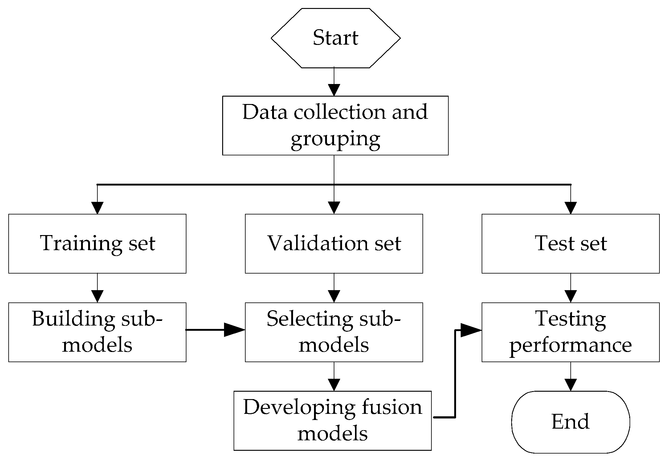
2.3. Implementation Steps

The preferred BP neural network, support vector machine and extreme learning machine sub-models are used to establish the prediction model by linear fusion method. This process is divided into three steps including data collection and grouping, sub-model training and evaluation, fusion model developing and testing. The implementation process is shown in Figure 1.

The implementation steps are as follows:

(1) Data collection and grouping

According to the modeling requirements, the dataset for modeling is collected. The whole dataset is divided into a training set (X₁), validation set (X₂) and test set (X₃) in the appropriate proportion. The training set (X₁) is selected in a way that covers all the ranges of the experimental data and operating conditions.

(2) Sub-model training and evaluation

The implementation process of sub-model training and evaluation is shown in Figure 2. Different types of sub-models are developed through training sets (X₁). The BP sub-models (BP-ANN₁, BP-ANN₂, …, BP-ANN_m) are established by changing the number of hidden layer nodes. The different types of kernel functions are chosen to develop SVM sub-models (SVM₁, SVM₂, …, SVM_n). Based on different hidden layer neurons and iterative functions, the ELM sub-models (ELM₁, ELM₂, …, ELM_k) are built. The model parameters are optimized by genetic algorithm (GA) to obtain the best results for each model.

The prediction performances of each sub-model are evaluated by using the validation set (X₂). According to the performance indicators of the validation set, the optimal sub-models are selected from the same kind of sub-models. Then, three optimal sub-models are obtained, which are BP-ANN_Opt, SVM_Opt, ELM_Opt.

(3) Fusion models developing and testing

The implementation process of the fusion model development and testing is shown in Figure 3. The parameters w₁, w₂ and w₃ represent the combination weight of three optimal sub-models, respectively. The weight of the three sub-models is calculated by the method of minimum square error (Equation (9)) or the information entropy method (Equation (16)) separately. Then, the two linear fusion models are established. Finally, the prediction performance of the built linear fusion models are tested using the test set (X₃).

3. Results and Discussion

3.1. Data Collecting and Grouping

The six important parameters of nine imidazole ionic liquids including temperature, pressure, critical temperature (Tc), critical pressure (Pc), molecular weight (M) and eccentricity factor (w) were taken as input variables of the prediction model. Theoretically, Tc, Pc, M and w are the essential thermodynamic properties of ILs. They can distinguish the species of ILs and reflect the characteristics of ionic liquid structures [20,34], which are listed in

Table 1. The properties of ionic liquids (ILs) in this study.

No.	Ionic Liquids	MW (g/mol)	Tc (k)	Pc (MPa)	Acentric Factor (w)
1	[BMIM][BF4]	226.03	623.3	2.04	0.8489
2	[EMIM][TF2N]	391.30	788.05	3.31	1.225
3	[EMIM][ETSO4]	236.29	1061.1	4.04	0.3368
4	[HMIM][TF2N]	447.92	1292.78	2.3888	0.3893
5	[HMIM][TFO]	316.34	1055.6	2.4954	0.489
6	[HMIM][BF4]	254.08	716.61	1.7941	0.6589
7	[HMIM][MESO4]	278.37	1110.84	2.9611	0.4899
8	[BMMIM][TF2N]	433.4	1255.8	2.031	0.3193
9	[HMIM][PF6]	312.24	759.16	1.5499	0.9385

. Temperature and CO₂ pressure will affect the solubility of CO₂ in the ionic liquid. For the same kind of ionic liquid, when the temperature decreases or the pressure increases, the solubility of CO₂ in the ionic liquid would increase. The solubility of CO₂ in ILs was chosen as the output variable of the model.

In order to develop dependable models, it is necessary to collect properties of CO₂ in different ILs from the literature. In this study, the 544 samples were collected and depicted partly in

Table 2. Input and output parameters used to construct models.

No.	Ionic Liquids	Temperature Range (K)	Pressure Range (MPa)	CO2 Solubility Range (Mole Fraction)	No. of Samples	Refs.
1	[BMIM][BF4]	278.47–368.22	0.587–67.620	0.102–0.602	104	[35,36]
2	[EMIM][TF2N]	312.10–410.90	0.626–14.329	0.123–0.593	77	[35,37]
3	[EMIM][ETSO4]	303.15–353.15	0.122–1.546	0.008–0.132	39	[35,38]
4	[HMIM][TF2N]	303.15–373.15	0.420–45.280	0.165–0.824	64	[20,39]
5	[HMIM][TFO]	303.15–373.15	1.420–100.120	0.267–0.816	64	[20,39]
6	[HMIM][BF4]	303.15–373.15	1.200–41.690	0.212–0.622	48	[20,39]
7	[HMIM][MESO4]	303.15–373.15	0.870–50.140	0.158–0.602	48	[20,39]
8	[BMMIM][TF2N]	298.15–343.15	0.010–1.900	0.002–0.211	36	[20,40]
9	[HMIM][PF6]	243.15–373.15	0.220–55.630	0.216–0.691	64	[20,39]

[20,35,36,37,38,39,40]. All the solubility of CO₂ in ionic liquids in this paper was obtained in the equilibrium phase. The unit of stoichiometry of reagents gas/ionic liquids is molar ratio. The dataset was randomly divided into three sets. A total of 70% of the sample named training set was used to generate the sub-models. A total of 15% of the sample named validation set was applied to select the best performance sub-models among the same kind of models. The other named test set was used to test the performance of the fusion model.

3.2. Fusion Model Development

3.2.1. Sub-Models Development

The sub-models of different structures were established by the training set. All sub-models were implemented by using MATLAB software (version 2016a, MathWorks, Natick, MA, United States). The details are as follows:

(1) The BP neural network with a single hidden layer can realize arbitrary mapping of continuous nonlinear function [41]. Thus, a series of BP neural network sub-models with different numbers of neurons (from 3 to 10 in sequence) in the hidden layer were established by using a three layers structure. In order to achieve nonlinear mapping, the transfer iterative function of the hidden layer is the Tansig function. The training algorithm uses the Levenberg–Marquardt Algorithm. To expand the range, the output layer uses the purelin iterative function.

(2) Three sub-models of SVM were established by choosing the polynomial kernel function, radial basis function and sigmoid function respectively. Genetic algorithm was incorporated to optimize the parameters of various kernel functions. The optimization result of the order of the polynomial in polynomial kernel function is 12. The optimized kernel width of the radial basis kernel function is 0.002. The optimized parameters of scalar and displacement of the Sigmoid function are 0.081 and −1.68, respectively.

(3) Eight extreme learning machine sub-models were established by selecting different hidden layer neurons and activation functions. Among them, the hidden layer nodes of five sub-models whose activation function is sigmoid were taken from 148 to 152 in turns. The hidden layer nodes of the other models with sine function were taken from 151 to 153 in order. The genetic algorithm was used to optimize the weight and threshold of each extreme learning machine sub-model.

3.2.2. Sub-Models Evaluation

The validation set was used to evaluate the performance of different types of sub-models. It screened out the optimal sub-models for model fusion. Four different statistical parameters of mean absolute error (MAE), root mean square error (RMSE), correlation coefficient (R²), and standard deviation (STD) were utilized (Equations (17)–(20)) to investigate the accuracy of the proposed models. The specific calculation formula for each indicator is as follows:

$$MAE=\frac{1}{N}{\displaystyle \sum _{i=1}^N\left|x_i-{\widehat{x}}_i\right|},$$

(17)

$$RMSE=\sqrt{\frac{{\displaystyle \sum _{i=1}^N{\left({\widehat{x}}_i-x_i\right)}^2}}{N}},$$

(18)

$$R^2=1-\frac{{\displaystyle \sum _{i=1}^N{\left({\widehat{x}}_i-x_i\right)}^2}}{{\displaystyle \sum _{i=1}^N{\left({\widehat{x}}_i-\overline{x}\right)}^2}},$$

(19)

$$STD={\displaystyle \sum _{i=1}^N{\left(\frac{x_i-\overline{x}}{N}\right)}^{0.5}},$$

(20)

where N is the number of samples, x_i is the predicted value of the sample i, ${\widehat{x}}_i$ is the true value of the sample i, $\overline{x}$ is the average of all samples.

The predictive performance of the each sub-model was obtained from the validation set. The result is shown in

Table 3. Performance of Back Propagation (BP) neural network sub-models.

No. of Hidden Layer Neurons	MAE	RMSE	R2	STD
3	0.0081	0.0114	0.9973	0.0659
4	0.0062	0.0085	0.9985	0.0499
5	0.0076	0.0099	0.9979	0.0616
6	0.0064	0.0088	0.9983	0.0521
7	0.0063	0.0090	0.9983	0.0512
8	0.0082	0.0108	0.9975	0.0661
9	0.0064	0.0092	0.9982	0.0521
10	0.0070	0.0096	0.9981	0.0567

. The BP neural network sub-model with four hidden layer neurons achieves the most accurate performance. The prediction effects of SVM sub-models with different kernel functions are indicated in

Table 4. Performance of Support Vector Machine (SVM) sub-models.

Type of Kernel Function	MAE	RMSE	R2	STD
Polynomial kernel function	0.0135	0.0196	0.9922	0.1091
Radial basis kernel function	0.0122	0.0180	0.9928	0.0992
Sigmoid kernel function	0.0269	0.0363	0.9727	0.2180

. The sub-model with the radial basis function has the least prediction error. As shown in

Table 5. Performance of Extreme Learning Machine (ELM) sub-models.

No. of Neurons	Type of Activation Function	MAE	RMSE	R2	STD
148	sigmoid	0.0124	0.0176	0.9970	0.1007
149	sigmoid	0.0106	0.0149	0.9938	0.0856
150	sigmoid	0.0113	0.0158	0.9959	0.0912
151	sigmoid	0.0112	0.0157	0.9940	0.0911
152	sigmoid	0.0120	0.0176	0.9928	0.0969
151	sine	0.0122	0.0182	0.9953	0.0989
152	Sine	0.0115	0.0166	0.9945	0.0928
153	sine	0.0113	0.0172	0.9933	0.0911

, the sub-model with 150 neurons in the hidden layer and sigmoid function reaches the optimal results.

3.2.3. Sub-Models Fusion

The weights of three screened sub-models were obtained by the method of minimizing the sum of squares error (Equation (9)). The expression of the linear fusion model is as follows:

$$Y=0.3630y_{BP}+0.2816y_{SVM}+0.3554y_{ELM},$$

(21)

where Y indicts the output of the linear fusion model; y_BP denotes the output of the BP neural network sub-model with the topology of 6 × 4 × 1; y_SVM represents the output of the SVM sub-model with the radial basis kernel function; y_ELM denotes the output of the ELM sub-model with the number of neurons in the hidden layer as 150 and the activation function is sigmoid.

Combining the same selected sub-models, the weights of each sub-model were calculated by using the information entropy method (Equation (16)). The output of the linear fusion model is as follows:

$$Y=0.3715y_{BP}+0.2689y_{SVM}+0.3596y_{ELM}.$$

(22)

3.3. Fusion Model Testing

The sub-models with better model performance were screened through the validation set. The fusion model established by the method of minimum squared error is the linear fusion model I, and the fusion model using the information entropy method is the linear fusion model II. The performance of the above five models mentioned above were tested by using the test set, and the prediction effects of the various models are shown in Figure 4.

In Figure 4, the horizontal and vertical axes are presented experimental and prediction values, respectively. The perfect fit is indicated by the solid line and the square points show the real predicted values. In other words, the closer the square points are to the solid lines the more accurate the correlation. Based on this definition, the results in Figure 4 show good correlative capability of the five models.

Figure 5 depicts the error histogram between the experimental values and the predicted values of each sub-model. The percentage of error distribution of each model is shown, and the fused model follows the normal distribution curve more effectively than the single sub-model. In this case, Figure 5 also proves the superiority of the fused models.

In order to quantitatively describe the prediction effects of the five models, the mean absolute error (MAE), root mean square error (RMSE), correlation coefficient (R²) and standard deviation (STD) of the five models in the test set are given in

Table 6. Performance indicators of five kinds of models.

Model	MAE	RMSE	R2	STD
BP	0.0068	0.0090	0.9982	0.0538
SVM	0.0105	0.0174	0.9933	0.0854
ELM	0.0093	0.0136	0.9961	0.0752
Linear fusion model I	0.0062	0.0090	0.9983	0.0533
Linear fusion model II	0.0060	0.0084	0.9985	0.0506

.

The error performance indicators of each model in Table 6 are shown in the form of a histogram in Figure 6. It can be seen more intuitively that the error performance indicators of two different linear fusion models are reduced compared with the optimal sub-models. By synthesizing all charts, it is proved that the linear fusion model has better prediction performance. As the linear fusion model can fully combine the characteristics of each sub-model and provide useful information for the prediction model from different perspectives, the accuracy and reliability of the prediction fusion model are improved.

In the two linear fusion models, the performance of the fusion model based on the information entropy method is better than that of the fusion model established by the method of minimum squared error. The weight of the fusion model is obtained by the method of minimum square error, which can reduce the model prediction error. However, this fusion model is susceptible to the samples, which leads to descent of global performance. The weight of the fusion model which is obtained by the information entropy method comprehensively considers the difference and error factors between the sub-models. The method can use the explicit and invisible information of the sample to disperse the prediction risk of the model, and then improve the prediction accuracy of the model.

4. Conclusions

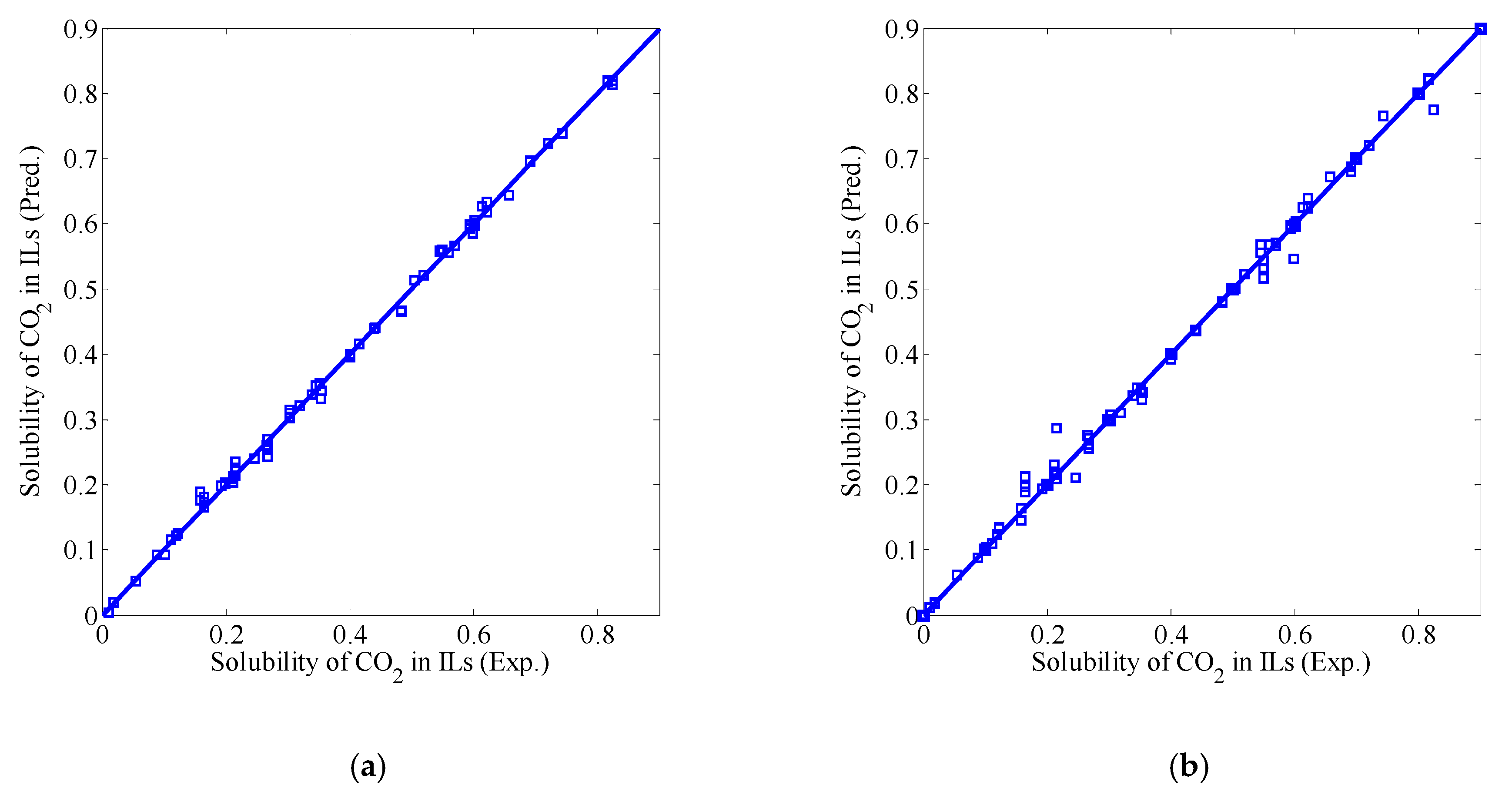
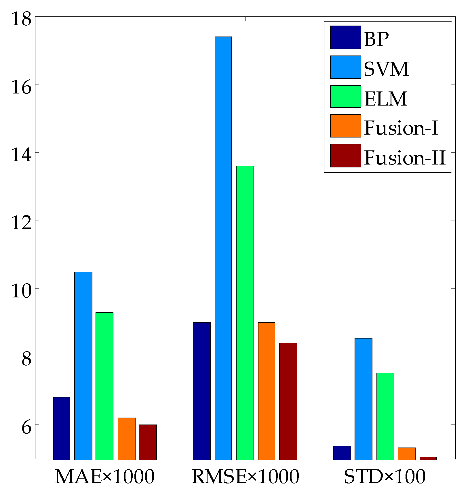
In this paper, a fusion modeling method was proposed for predicting the solubility of CO₂ in ILs. Firstly, 544 sets of samples from nine ILs were collected from the literature, and divided into a training set, validation set and test set according to a certain proportion. The sub-models of the BP neural network, SVM and ELM were established by using the training set. Among them, three sub-models with the optimal evaluation performance were selected by using the validation set. Then, the linear fusion models were established by using the minimum square error method and the information entropy method, respectively. Finally, the test set was used to test the prediction performance of the linear fusion models and optimal sub-models. The results show that the prediction effect of the linear fusion model is better than other single sub-models. Furthermore, the prediction effect of the linear fusion model based on the information entropy method is better than based on the minimum square error method.

Although the prediction model established by the fusion modeling method has a good prediction effect of nine imidazole ionic liquids in the paper, it may not be suitable for the prediction of the solubility of other ILs in CO₂. Nonetheless, the fusion modeling method solves the shortcomings of being time-consuming, high cost of experimental measurement and the complexity and generalization of mechanism model. It provides an effective method for predicting the solubility of CO₂ in the ILs, and also can be considered as a new method for prediction of different thermodynamic properties.

References

1. Zhao, Z.J.; Dong, H.F.; Zhang, X.P. The research progress of CO2 capture with ionic liquids. Chin. J. Chem. Eng. 2012, 20, 120–129. [Google Scholar] [CrossRef]
2. Zhang, S.J.; Liu, X.M.; Yao, X.Q.; Dong, H.F.; Zhang, X.P. Frontiers, progresses and applications of ionic liquids. Sci. China 2009, 39, 1134–1144. [Google Scholar]
3. Bara, J.E.; Gin, D.L.; Noble, R.D. Effect of anion on gas separation performance of polymer-room-temperature ionic liquid composite membranes. Ind. Eng. Chem. Res. 2008, 47, 9919–9924. [Google Scholar] [CrossRef]
4. Abejón, R.; Rabadán, J.; Lanza, S.; Abejón, A.; Garea, A.; Irabien, A. Supported ionic liquid membranes for separation of lignin aqueous solutions. Processes 2018, 6, 143. [Google Scholar] [CrossRef]
5. Brennecke, J.F.; Gurkan, B.E. Ionic liquids for CO2 capture and emission reduction. J. Phys. Chem. Lett. 2017, 1, 3459–3464. [Google Scholar] [CrossRef]
6. Gurkan, B.; Goodrich, B.F.; Mindrup, E.M.; Ficke, L.E.; Masse, M.; Seo, S.; Senftle, T.P.; Wu, H.; Glaser, M.F.; Shah, J.K.; et al. Molecular design of high capacity, low viscosity, chemically tunable ionic liquids for CO2 capture. J. Phys. Chem. Lett. 2017, 1, 3494–3499. [Google Scholar] [CrossRef]
7. Bahmani, A.R.; Sabzi, F.; Bahmani, M. Prediction of solubility of sulfur dioxide in ionic liquids using artificial neural network. J. Mol. Liq. 2015, 211, 395–400. [Google Scholar] [CrossRef]
8. Ding, J.; Xiong, Y.; Yu, D.H. Solubility of CO2 in ionic liquids—measuring and modeling methods. Chem. Ind. Eng. Prog. 2012, 31, 732–741. [Google Scholar]
9. Jaubert, J.N.; Vitu, S.; Mutelet, F. Extension of the PPR78 model (predictive 1978, Peng-Robinson EOS with temperature dependent kij calculated through a group contribution method) to systems containing aromatic compounds. Fluid Phase Equilibr. 2006, 237, 193–211. [Google Scholar] [CrossRef]
10. Lei, Z.G.; Dai, C.N.; Chen, B.H. Gas solubility in ionic liquids. Chem. Rev. 2014, 114, 1289–1326. [Google Scholar] [CrossRef]
11. Soave, G. Equilibrium constants from a modified Redlich-Kwong equation of state. Chem. Eng. Sci. 1972, 27, 1197–1203. [Google Scholar] [CrossRef]
12. Breure, B.; Bottini, S.B.; Witkamp, G.J.; Peters, C.J. Thermodynamic modeling of the phase behavior of binary systems of ionic liquids and carbon dioxide with the group contribution equation of state. J. Phys. Chem. B 2007, 111, 14265–14270. [Google Scholar] [CrossRef]
13. Carvalho, P.J.; Álvarez, V.H.; Marrucho, I.M.; Aznar, M.; Coutinho, J.P. High pressure phase behavior of carbon dioxide in 1-butyl-3-methylimidazolium bis(trifluoromethylsulfonyl)imide and 1-butyl-3-methylimidazolium dicyanamide ionic liquids. J. Supercrit. Fluid. 2009, 50, 105–111. [Google Scholar] [CrossRef]
14. Bavoh, C.B.; Lal, B.; Nashed, O.; Khan, M.S.; Keong, L.K.; Bustam, M.A. COSMO-RS: An ionic liquid prescreening tool for gas hydrate mitigation. Chin. J. Chem. Eng. 2016, 24, 1619–1624. [Google Scholar] [CrossRef]
15. Gholizadeh, A.; Sabzi, F. Prediction of CO2 sorption in poly(ionic liquid)s using ANN-GC and ANFIS-GC models. Int. J. Greenh. Gas Con. 2017, 63, 95–106. [Google Scholar] [CrossRef]
16. Ghiasi, M.M.; Mohammadi, A.H. Application of decision tree learning in modelling CO2 equilibrium absorption in ionic liquids. J. Mol. Liq. 2017, 242, 594–605. [Google Scholar] [CrossRef]
17. Eslamimanesh, A.; Gharagheizi, F.; Mohammadi, A.H.; Richon, D. Artificial Neural Network modeling of solubility of supercritical carbon dioxide in 24 commonly used ionic liquids. Chem. Eng. Sci. 2011, 66, 3039–3044. [Google Scholar] [CrossRef]
18. Lashkarbolooki, M.; Shafipour, Z.S.; Hezave, A.Z.; Farmani, H. Use of artificial neural networks for prediction of phase equilibria in the binary system containing carbon dioxide. J. Supercrit. Fluid. 2013, 75, 144–151. [Google Scholar] [CrossRef]
19. Lashkarbolooki, M.; Shafipour, Z.S.; Hezave, A.Z. Trainable cascade-forward back-propagation network modeling of spearmint oil extraction in a packed bed using SC-CO2. J. Supercrit. Fluid. 2013, 73, 108–115. [Google Scholar] [CrossRef]
20. Tatar, A.; Naseri, S.; Bahadori, M.; Hezave, A.Z.; Kashiwao, T.; Bahadori, A.; Darvish, H. Prediction of carbon dioxide solubility in ionic liquids using MLP and radial basis function (RBF) neural networks. J. Taiwan Inst. Chem. E. 2016, 60, 151–164. [Google Scholar] [CrossRef]
21. Yang, Y.; Chen, Y.H.; Wang, Y.C.; Li, C.H.; Li, L. Modelling a combined method based on ANFIS and neural network improved by DE algorithm: A case study for short-term electricity demand forecasting. Appl. Soft Comput. 2016, 49, 663–675. [Google Scholar] [CrossRef]
22. Zuan, P.; Huang, Y. Prediction of sliding slope displacement based on intelligent algorithm. Wirel. Pers. Commun. 2018, 102, 3141–3157. [Google Scholar] [CrossRef]
23. Xu, Q.; Chen, J.Y.; Liu, X.P.; Li, J.; Yuan, C.Y. An ABC-BP-ANN algorithm for semi-active control for magnetorheological damper. KSCE J. Civ. Eng. 2017, 21, 2310–2321. [Google Scholar] [CrossRef]
24. Sridhar, D.V.; Bartlett, E.B.; Seagrave, R.C. Information theoretic subset selection for neural network models. Comput. Chem. Eng. 1998, 22, 613–626. [Google Scholar] [CrossRef]
25. Tatar, A.; Yassin, M.R.; Rezaee, M.; Aghajafari, A.H.; Shokrollahi, H. Applying a robust solution based on expert systems and GA evolutionary algorithm for prognosticating residual gas saturation in water drive gas reservoirs. J. Nat. Gas Sci. Eng. 2014, 21, 79–94. [Google Scholar] [CrossRef]
26. Ling, H.; Qian, C.; Kang, W.; Liang, C.; Chen, H. Combination of Support Vector Machine and K-Fold cross validation to predict compressive strength of concrete in marine environment. Constr. Build. Mater. 2019, 206, 355–363. [Google Scholar] [CrossRef]
27. Zhou, T.; Lu, H.; Wang, W.W.; Yong, X. GA-SVM based feature selection and parameter optimization in hospitalization expense modeling. Appl. Soft Comput. 2019, 75, 323–332. [Google Scholar]
28. Huang, G.B.; Zhu, Q.Y.; Siew, C.K. Extreme learning machine: Theory and applications. Neurocomputing 2006, 70, 489–501. [Google Scholar] [CrossRef]
29. Lan, Y.; Soh, Y.C.; Huang, G.B. Ensemble of online sequential extreme learning machine. Neurocomputing 2009, 72, 3391–3395. [Google Scholar] [CrossRef]
30. Huang, G.B.; Ding, X.J.; Zhou, H.M. Optimization method based extreme learning machine for classification. Neurocomputing 2010, 74, 155–163. [Google Scholar] [CrossRef]
31. Wang, S.H.; Li, H.F.; Zhang, Y.J.; Zou, Z.S. A hybrid ensemble model based on ELM and improved AdaBoost.RT algorithm for predicting the iron ore sintering characters. Comput. Intel. Neurosc. 2019, 60, 1–11. [Google Scholar] [CrossRef] [PubMed]
32. Kurnaz, T.F.; Kaya, Y. The comparison of the performance of ELM, BRNN, and SVM methods for the prediction of compression index of clays. Arab. J. Geosci. 2018, 11, 1–14. [Google Scholar]
33. Shannon, C.E. A mathematical theory of communication. Bell Labs Tech. J. 1948, 27, 379–423. [Google Scholar] [CrossRef]
34. Baghban, A.; Ahmadi, M.A.; Shahraki, B.H. Prediction carbon dioxide solubility in presence of various ionic liquids using computational intelligence approaches. J. Supercrit. Fluid. 2015, 98, 50–64. [Google Scholar] [CrossRef]
35. Sedghamiz, M.A.; Rasoolzadeh, A.; Rahimpour, M.R. The ability of artificial neural network in prediction of the acid gases solubility in different ionic liquids. J. CO2 Util. 2015, 9, 39–47. [Google Scholar] [CrossRef]
36. Haghbakhsh, R.; Soleymani, H.; Raeissi, S. A simple correlation to predict high pressure solubility of carbon dioxide in 27 commonly used ionic liquids. J. Supercrit. Fluid. 2013, 77, 158–166. [Google Scholar] [CrossRef]
37. Schilderman, A.M.; Raeissi, S.; Peters, C.J. Solubility of carbon dioxide in the ionic liquid 1-ethyl-3-methylimidazolium bis(trifluoromethylsulfonyl)imide. Fluid Phase Equilibr. 2007, 260, 19–22. [Google Scholar] [CrossRef]
38. Jalili, A.H.; Mehdizadeh, A.; Shokouhi, M.; Ahmadi, A.N.; Fateminassab, F. Solubility and diffusion of CO2 and H2S in the ionic liquid 1-ethyl-3-methylimidazolium ethylsulfate. J. Chem. Thermodyn. 2010, 42, 1298–1303. [Google Scholar] [CrossRef]
39. Lashkarbolooki, M.; Vaferi, B.; Rahimpour, M.R. Comparison the capability of artificial neural network (ANN) and EOS for prediction of solid solubilities in supercritical carbon dioxide. Fluid Phase Equilibr. 2011, 308, 35–43. [Google Scholar] [CrossRef]
40. Tagiuri, A.; Sumon, K.Z.; Henni, A. Solubility of carbon dioxide in three [Tf2N] ionic liquids. Fluid Phase Equilibr. 2014, 380, 39–47. [Google Scholar] [CrossRef]
41. Cybenko, G. Approximation by superpositions of a sigmoidal function. Math. Control Signal. 1992, 5, 455. [Google Scholar] [CrossRef]
Figure 1. The flowchart of developing multi-model fusion models.
Processes 07 00258 g001
Figure 2. The steps of sub-model training and evaluation.
Processes 07 00258 g002
Figure 3. The flowchart of fusion models developing and testing.
Processes 07 00258 g003
Figure 4. Experimental data versus models results: (a) BP, (b) SVM, (c) ELM, (d) linear fusion model I, and (e) linear fusion model II.
Processes 07 00258 g004aProcesses 07 00258 g004b
Figure 5. Histogram of error distribution for CO2 solubility in ILs prediction by proposed model. (a) BP, (b) SVM, (c) ELM, (d) linear fusion model I and (e) linear fusion model II.
Processes 07 00258 g005
Figure 6. Comparison of different performance indicators of each model.
Processes 07 00258 g006