Convergence of Subtangent-Based Relaxations of Nonlinear Programs

Abstract

Convex relaxations of functions are used to provide bounding information to deterministic global optimization methods for nonconvex systems. To be useful, these relaxations must converge rapidly to the original system as the considered domain shrinks. This article examines the convergence rates of convex outer approximations for functions and nonlinear programs (NLPs), constructed using affine subtangents of an existing convex relaxation scheme. It is shown that these outer approximations inherit rapid second-order pointwise convergence from the original scheme under certain assumptions. To support this analysis, the notion of second-order pointwise convergence is extended to constrained optimization problems, and general sufficient conditions for guaranteeing this convergence are developed. The implications are discussed. An implementation of subtangent-based relaxations of NLPs in Julia is discussed and is applied to example problems for illustration.

1. Introduction

Many process engineering problems may be formulated and approached as optimization problems. Typical examples include seeking optimal operating conditions for combined cooling, heating, and power (CCHP) systems [1,2,3]; seeking optimal schedules for thermal power plants [4,5]; and maximizing recovered energy in heat-waste recovery systems [6,7], subject to thermodynamic and financial constraints.

Process models may exhibit significant nonconvexity, making them challenging to analyze, simulate, and optimize. For example, periodic trigonometric functions are often employed to estimate the total incident radiation in solar power generation systems [8]. In crude-oil scheduling problems, bilinear terms are typically used to model constraints involving compositions of mixtures transferred from holding tanks [9]. In the modeling of counterflow heat exchangers, logarithmic mean temperatures are generally used to describe the temperature difference between hot and cold streams [10]. Individual process units such as compressors [11] and hydroelectric generators [12] are often modeled using nonconvex correlations. Moreover, models of thermodynamic properties often introduce nonconvexity; such models include the Peng–Robinson equation of state [13], the Antoine equation, and descriptions of the dependence of heat capacity on temperature [7]. Physical property models involving empirical correlations may also introduce nonconvexities through fractional or logarithmic terms, such as models of heat transfer coefficients [14] and friction factors in fluid mechanics [11].

Due to the size and nonconvexity of chemical process models, stochastic global search algorithms [15] are often used in practice to optimize them; such methods include genetic algorithms [16], differential evolution algorithms [17], and particle swarm algorithms [18]. However, these heuristic methods will typically only locate a suboptimal local minimum in finite time. Compared with a suboptimal local optima, a global optimum represents a more desirable outcome, such as the lowest operating cost, the highest profit, or the most efficient heat integration. Moreover, in several optimization applications, suboptimal local minima are inappropriate and global optimization is essential. Such problems include parameter estimation problems for energy models [19], design centering problems [20], and worst-case uncertainty analysis [21] involving either a probabilistic risk analysis [22] or a safety verification analysis [23]. Parameter estimation aims to choose parameters to minimize the difference between the prediction of a model and experiment data, and global optimization can confirm that a particular model is inappropriate regardless of parameter choice. A worst-case uncertainty analysis determines the maximal possible cost based on an assessment of the probability distribution of parameter values.

Since stochastic global search algorithms will not typically locate a global optimum in finite time, we instead focus on deterministic global optimization methods such as branch and bound [24], which guarantee that the global minimum will be located in finite time to within a prespecified tolerance. Branch-and-bound methods employ upper and lower bounds of objective functions, which are refined progressively as the decision space is subdivided, until the bounds converge to within a specified tolerance. When applied to minimization problems, upper bounds are typically furnished as local minima obtained by local NLP solvers. Computing lower bounds, on the other hand, requires global knowledge of the model and constraints and are typically obtained by replacing the objective function and constraints by convex relaxations. The local optimization of these relaxations yields lower bounds for the original problem. The convex relaxations supplied to a branch-and-bound method must converge rapidly to the underlying model as the decision space is subdivided or else the overall global optimization method will be impeded by cluster effects [25]. This notion of rapid convergence has been formalized as a second-order pointwise convergence [26,27].

Several established approaches can be used to generate convex relaxations automatically, including $\alpha$BB relaxations [28,29], and McCormick relaxations [30,31,32,33,34], all of which exhibit second-order pointwise convergence under mild assumptions [26,35]. However, obtaining lower bounds by minimizing these relaxations can be expensive due to their nonlinearity. This article considers relaxing nonlinear relaxations to piecewise-affine relaxations, which are weaker than the underyling nonlinear relaxations but may be optimized inexpensively as linear programs. In this approach, one first constructs subtangents of the nonlinear relaxations at linearization points which sample the decision space. Then, piecewise-affine relaxations are constructed as the pointwise maximum of all considered subtangents, and minimized using standard linear-program solvers to generate lower-bounding information. These piecewise-affine relaxations are shown to inherit second-order pointwise convergence from the nonlinear relaxations in certain cases, extending recent results concerning affine relaxations [36]. Thus, in these cases, the piecewise-affine relaxations can converge rapidly enough to the underlying systems as the decision space is subdivided to be useful in methods for deterministic global optimization. To support this analysis, a useful notion of second-order pointwise convergence is developed for general optimization problems with nontrivial constraints; sufficient conditions are provided under which this convergence is guaranteed; and a counterexample is presented, showing that a convergence may fail if these sufficient conditions are not satisfied. This convergence framework for constrained optimization problems complements existing convergence results [37], which determine the effect of including additional linearization points rather than shrinking the underlying domain, and may be used in concert with recent techniques [34] to obtain tighter relaxations of individual functions by leveraging subtangents in a different way. Moreover, it complements previous work concerning second-order pointwise convergence [26,27,35,36,38], which does not consider optimization problems with nontrivial constraints.

This article makes the following contributions. First, sufficient conditions are presented for the second-order pointwise convergence of piecewise-affine outer approximations that are based on subgradients of an underlying convex relaxation scheme. These sufficient conditions are straightforward to check and, thereby, provide a useful and novel guarantee that a broad class of outer approximation methods will not introduce clustering into a branch-and-bound method for global optimization. Practical recommendations for constructing appropriate piecewise-affine relaxations are discussed. Second, these sufficient conditions are extended to nonlinear programs (NLPs) with nontrivial constraints. It is shown that these constraints can introduce pathological behavior; this behavior is shown nontrivially to be suppressed once sufficiently strong regularity assumptions are imposed. This development is, to our knowledge, the first discussion of a second-order pointwise convergence for optimization problems with nontrivial constraints. Third, the discussed relaxation approaches are implemented in Julia [39], and it is shown through several numerical examples that even a simple branch-and-bound method based on the described piecewise-affine relaxations can compete with the state-of-the-art.

The remainder of this article is structured as follows. Section 2 summarizes relevant established results and methods, including a recent result [36] concerning subtangent convergence. Section 3 extends this result to piecewise-affine relaxations based on subtangents, thus demonstrating their rapid convergence to the underlying system. The notion of second-order pointwise convergence is extended to constrained optimization problems in a useful sense, and sufficient conditions are developed under which this convergence is guaranteed. Practical considerations when constructing piecewise-affine relaxations are discussed. Section 4 places the results of this article in context with outer approximation methods [40,41,42] and recent subtangent-based tightening methods [34]. Section 5 presents an implementation of this article’s approximation approach in the language Julia; this implementation is applied to various test problems for illustration.

2. Background

Relevant definitions and established results are summarized in this section. Throughout this article, scalars are denoted as lowercase letters (e.g., p), vectors are denoted as boldfaced lowercase letters (e.g., $\mathbf{z}$), their components are denoted with subscripts (e.g., $z_i$), inequalities involving vectors are to be interpreted component-wise, sets are denoted as uppercase letters (e.g., Q), and the standard Euclidean norm $\parallel ·\parallel$ and inner product $\langle ·,·\rangle$ are employed.

2.1. Branch-and-Bound Optimization Using Convex Relaxations

Branch-and-bound methods [24,43,44] are deterministic global optimization algorithms that guarantee the location of a global minimum for a nonlinear program (NLP) to within a specified tolerance. These methods proceed by evaluating upper and lower bounds of the objective function, which are refined progressively as the domain is subdivided. Along the way, knowledge concerning the feasibility and the best bounds determined thus far may be used to exclude certain subdomains from consideration. Once the best bounds are equal up to the specified tolerance, the method terminates successfully.

From here, only continuous problems are considered. If branch-and-bound is applied to such a minimization problem, the supplied upper bounds can be any local minima obtained by local NLP solvers. Furnishing appropriate lower bounds, on the other hand, requires global knowledge of the model and constraints. A common approach is to replace the objective function and constraints with convex relaxations, which are underestimators that are convex and, therefore, relatively easy to minimize to global optimality using local methods. Thus, the local optimization of a convex relaxation yields a lower bound for the original problem. Several established methods may be used to generate convex relaxations, such as McCormick relaxations [30,31], $\alpha$BB relaxations [28,29], and relaxations obtained by Auxiliary Variable Methods [45]. Each of these relaxation schemes can be called a scheme of convex relaxations, as defined below.

Definition 1

(from Bompadre and Mitsos [26]). Let $Q\subset {\mathbb{R}}^n$ be a nonempty compact set and $f:Q\to \mathbb{R}$ be a continuous function, and define $\mathbb{I}Q:={\mathbb{IR}}^n\cap Q$. Suppose that, for each interval $W\in \mathbb{I}Q$, a function ${\underline{f}}_W^C:W\to \mathbb{R}$ is convex and underestimates f on W. Then, the collection ${\{{\underline{f}}_W^C\}}_{W\in \mathbb{I}Q}$ is a scheme of convex relaxations of f on Q.

2.2. Convergence of Convex Relaxation Schemes

The following definition from Bompadre and Mitsos [26] formalizes a notion of the convex relaxations of a function approaching that function rapidly as the underlying subdomain shrinks.

Definition 2.

Given a function $f:Q\to \mathbb{R}$ and a scheme of convex relaxations ${\{{\underline{f}}_W^C\}}_{W\in \mathbb{I}Q}$ of f on Q as in Definition 1, this scheme has second-order pointwise convergence if there exists a constant $\tau >0$ such that, for each interval $W\in \mathbb{I}Q,$

$$\underset{\mathbf{z}\in W}{sup}\left(f\left(\mathbf{z}\right)-{\underline{f}}_W^C\left(\mathbf{z}\right)\right)\le \tau {\left(\mathrm{wid}W\right)}^2,$$

where $\mathrm{wid}W:=max\{|{\overline{w}}_i-{\underline{w}}_i|:1\le i\le n\}$ is the width of W.

Second-order pointwise convergence is beneficial in global optimization to avoid cluster effects [25,27], in which a branch-and-bound method must divide excessively often on subdomains that include or are near a global minimum.

Established results [26,35,38] show that several established methods for generating convex relaxation schemes produce schemes with second-order pointwise convergence. These methods include auxiliary variable methods [45], $\alpha$BB relaxations [28], classic McCormick relaxations [26], multivariate McCormick relaxations [32], and differentiable McCormick relaxations [38].

2.3. Subtangents of Convex Relaxations

Standard definitions of subtangents, subgradients, and subdifferentials for convex functions are as follows.

Definition 3

(adapted from Rockafellar [46]). Given a convex set $Z\subset {\mathbb{R}}^n$ and a convex function $\varphi :Z\to \mathbb{R}$, a vector $\mathbf{s}\in {\mathbb{R}}^n$ is a subgradient of $\varphi$ at $\mathit{\zeta }\in Z$ if

$$\varphi \left(\mathbf{z}\right)\ge \varphi \left(\mathbf{\zeta }\right)+\langle \mathbf{s},\mathbf{z}-\mathbf{\zeta }\rangle ,\forall \mathbf{z}\in Z,$$

in which case the affine mapping $\mathbf{z}\mapsto \varphi \left(\mathit{\zeta }\right)+\langle \mathbf{s},\mathbf{z}-\mathit{\zeta }\rangle$ is a subtangent of $\varphi$ at $\mathit{\zeta }$. The subdifferential $\partial \varphi \left(\mathit{\zeta }\right)\subset {\mathbb{R}}^n$ is the collection of all subgradients of $\varphi$ at $\mathit{\zeta }$.

Consider a particular convex relaxation scheme with second-order pointwise convergence. A recent result by Khan [36] showed that, although any convex relaxation dominates all of its subtangents, subtangents for this relaxation scheme will nevertheless inherit the second-order pointwise convergence under mild assumptions. This result is reproduced below; it employs the constructions in the following definition and assumption.

Definition 4

(from Khan [36]). For any interval $W:=[\underline{\mathbf{w}},\overline{\mathbf{w}}]\in {\mathbb{IR}}^n$, denote the midpoint of W as ${\mathbf{w}}^{\mathrm{mid}}:=\frac{1}{2}(\underline{\mathbf{w}}+\overline{\mathbf{w}})\in W$. For any $\alpha \in [0,+\infty )$, define a centrally-scaled interval of W as

$${\mathbf{s}}_{\alpha }\left(W\right):=\{{\mathbf{w}}^{\mathrm{mid}}\}+\alpha (W-\{{\mathbf{w}}^{\mathrm{mid}}\}),$$

where the addition and subtraction are in the sense of Minkowski.

Observe that ${\mathbf{w}}^{\mathrm{mid}}\in {\mathbf{s}}_{\alpha }\left(W\right)$ regardless of the value of $\alpha$.

Assumption 1.

Consider a nonempty open set $Z\subset {\mathbb{R}}^n$ and a function $f:Z\to \mathbb{R}$ of which the gradient $\nabla f$ exists on Z and is locally Lipschitz continuous.Let $Q\subset Z$ be a nonempty compact set, and suppose that a scheme of convex relaxations ${\{{\underline{f}}_W^C\}}_{W\in \mathbb{I}Q}$ of f on Q has a second-order pointwise convergence.

Theorem 1

(adapted from Khan [36]). Suppose that Assumption 1 holds, and choose some $\alpha \in [0,1)$. For each $W\in \mathbb{I}Q$, choose some ${\mathit{\zeta }}_W\in {\mathbf{s}}_{\alpha }\left(W\right)$ and a subgradient ${\mathit{\sigma }}_W\in \partial {\underline{f}}_W^C\left(\mathit{\zeta }\right)$, and consider a subtangent ${\underline{f}}_{\mathrm{sub},W}^C:W\to \mathbb{R}$ of f on W with

$${\underline{f}}_{\mathrm{sub},W}^C\left(\mathbf{z}\right)\equiv {\underline{f}}_W^C\left(\mathbf{\zeta }\right)+\langle {\mathbf{\sigma }}_W,\mathbf{z}-\mathbf{\zeta }\rangle .$$

Then, ${\{{\underline{f}}_{\mathrm{sub},W}^C\}}_{W\in \mathbb{I}Q}$ is also a scheme of convex relaxations of f on Q with a second-order pointwise convergence.

Observe that this theorem does not place any differentiability requirements on the underestimators ${\underline{f}}_W^C$ and does not require the twice-continuous differentiability of f. Choosing each ${\mathit{\zeta }}_W$ to be an element of ${\mathbf{s}}_{\alpha }\left(W\right)$ rather than W is crucial; Khan [36] presents a counterexample in which second-order pointwise convergence is not obtained when this requirement is violated. Nevertheless, Khan [36] also shows that if the entire scheme of convex relaxations is uniformly continuously differentiable in a certain sense, then we may replace ${\mathbf{s}}_{\alpha }\left(W\right)$ with W without affecting the conclusion of Theorem 1.

3. New Convergence Results

This section extends the second-order pointwise convergence result of Theorem 1 to piecewise-affine outer approximations of functions and nonlinear programs (NLPs), as the underlying domain is reduced in size. This result complements an analysis by Rote [37], who considered the effect on convergence of including additional cutting planes rather than shrinking the domain. Sufficient conditions for a second-order pointwise convergence of NLPs with nontrivial constraints are also developed and presented.

3.1. Relaxations of Functions

To proceed, we must first strengthen Assumption 1.

Assumption 2.

Suppose that Assumption 1 holds and that the convex relaxations ${\underline{f}}_W^C$ are Lipschitz continuous on their respective domains.

Definition 5.

Suppose that Assumption 2 holds, and consider some $\alpha \in [0,1)$. For each interval $W\in \mathbb{I}Q$, choose a point ${\mathit{\zeta }}_W\in {\mathbf{s}}_{\alpha }\left(W\right)$ and a subset $B_W\subset W$. Define a subgradient-cutting mapping:

$${\underline{f}}_{\mathrm{cut},W}^C:=\mathbf{z}\mapsto max\{{\underline{f}}_W^C\left(\mathbf{\zeta }\right)+\langle {\mathbf{\sigma }}_W\left(\mathbf{\zeta }\right),\mathbf{z}-\mathbf{\zeta }\rangle :\mathbf{\zeta }\in B_W\cup \{{\mathbf{\zeta }}_W\}\},$$

(1)

where, in each case, ${\mathit{\sigma }}_W\left(\mathit{\zeta }\right)$ is a finite subgradient of ${\underline{f}}_W^C$ at $\mathit{\zeta }$.

Observe that any subgradient-cutting mapping ${\underline{f}}_{\mathrm{cut},W}^C$ is convex, since it is a pointwise maximum of affine functions. Moreover, it is an underestimator of both ${\underline{f}}_W^C$ and f on W, since it is the pointwise maximum of underestimators. Thus, ${\{{\underline{f}}_{\mathrm{cut},W}^C\}}_{W\in \mathbb{I}Q}$ is a scheme of convex relaxations of f on Q. If $B_W$ is finite, then ${\underline{f}}_{\mathrm{cut},W}^C$ is additionally piecewise affine. The following corollary of Theorem 1 provides a new convergence result for polyhedral outer approximations, by showing that subgradient-cutting mappings inherit a second-order pointwise convergence.

Theorem 2.

Suppose that Assumption 2 holds, choose some $\alpha \in [0,1)$, and consider a scheme ${\{{\underline{f}}_{\mathrm{cut},W}^C\}}_{W\in \mathbb{I}Q}$ of subgradient-cutting convex relaxations as in Definition 5. The scheme ${\{{\underline{f}}_{\mathrm{cut},W}^C\}}_{W\in \mathbb{I}Q}$ has a second-order pointwise convergence.

Proof. 

For each $W\in \mathbb{I}Q$, observe that ${\underline{f}}_{\mathrm{cut},W}^C$ dominates the affine mapping

$$\mathbf{z}\mapsto {\underline{f}}_W^C\left({\mathbf{\zeta }}_W\right)+\langle {\mathbf{\sigma }}_W\left({\mathbf{\zeta }}_W\right),\mathbf{z}-{\mathbf{\zeta }}_W\rangle$$

on W, which is a valid choice of ${\underline{f}}_{\mathrm{sub},W}^C$ in Theorem 1. Since ${\mathit{\zeta }}_W^0\in {\mathbf{s}}_{\alpha }\left(W\right)$ in each case, it follows that, for each $W\in \mathbb{I}Q$ and each $\mathbf{z}\in W$,

$$f\left(\mathbf{z}\right)-{\underline{f}}_{\mathrm{cut},W}^C\left(\mathbf{z}\right)\le f\left(\mathbf{z}\right)-{\underline{f}}_{\mathrm{sub},W}^C\left(\mathbf{z}\right).$$

The claim then follows from Theorem 1. ☐

3.2. Relaxations of Constrained Optimization Problems

Established definitions and analyses concerning second-order pointwise convergence [26,27,35,36,38] have focused on applications in global optimization problems with only bound constraints. To extend this analysis, this section considers the second-order pointwise convergence of optimization problems with nontrivial inequality constraints and applies Theorem 2 to handle piecewise-affine relaxations. Equality constraints may be regarded similarly, though with some care. As Example 1 below will illustrate, nontrivial constraints introduce obstacles to analysis that are not present in the box-constrained case, and must be circumvented by enforcing additional assumptions.

This section considers optimization problems that are represented as constrained nonlinear programming problems (NLPs) as follows.

Assumption 3.

Suppose that Assumption 1 holds, and that it also holds with each component $g_i$ of a function $\mathbf{g}:Z\to {\mathbb{R}}^m$ in place of f and with a scheme ${\{{\underline{g}}_{i,W}^C\}}_{W\in \mathbb{I}Q}$ in place of ${\{{\underline{f}}_W^C\}}_{W\in \mathbb{I}Q}$. For each set $W\in \mathbb{I}Q$, suppose that ${\underline{f}}_W^C$ and each ${\underline{g}}_{i,W}^C$ are Lipschitz continuous on W. Let F denote the collection of all sets $W\in \mathbb{I}Q$ for which there exists $\mathbf{z}\in W$ that satisfies $\mathbf{g}\left(\mathbf{z}\right)\le \mathbf{0}$, and assume that F is nonempty.

Supposing that Assumption 3 holds, consider the following NLP for each $W\in F$. (Here “subject to” is abbreviated as “s.t.”.)

$$\begin{array}{cc}\hfill \underset{\mathbf{z}\in W}{min}& f\left(\mathbf{z}\right)\hfill \\ \hfill \mathrm{s}.\mathrm{t}.& \mathbf{g}\left(\mathbf{z}\right)\le \mathbf{0}.\hfill \end{array}$$

(2)

For each $W\in F$, Weierstrass’s Theorem implies the NLP (2) has at least one solution and has a finite optimal objective function value $v\left(W\right)$. Replacing the objective function and constraints in (2) by the convex underestimators provided in Assumption 3, we obtain the following auxiliary NLP.

$$\begin{array}{cc}\hfill \underset{\mathbf{z}\in W}{min}& {\underline{f}}_W^C\left(\mathbf{z}\right)\hfill \\ \hfill \mathrm{s}.\mathrm{t}.& {\underline{g}}_{i,W}^C\left(\mathbf{z}\right)\le 0,\forall i=\{1,\dots ,m\}.\hfill \end{array}$$

(3)

Again, Weierstrass’s Theorem implies the convex NLP (3) has at least one solution and has a finite optimal objective function value $\underline{v}\left(W\right)$. Since the objective function and constraints of Equation (2) were replaced in (3) by underestimators, (3) is a relaxation of (2) in that $\underline{v}\left(W\right)\le v\left(W\right)$ for each $W\in F$. Such relaxations are commonly employed in deterministic methods for constrained global optimization [44]. Equality constraints in (2) may be relaxed analogously by replacing them with inequalities involving a convex underestimator and a concave overestimator; this was not presented here for simplicity.

We will explore conditions under which second-order pointwise convergence of the schemes of underestimators for f and $g_i$ in Assumption 3 translate to second-order pointwise convergence of (3) to (2), in the following sense.

Definition 6.

Suppose that Assumption 3 holds, and consider the optimal-value mappings v and $\underline{v}$ as defined above. Over all $W\in F$, the relaxed NLP (3) exhibits second-order pointwise convergence to the original NLP (2) if there exists ${\tau }_v>0$ for which

$$0\le v\left(W\right)-\underline{v}\left(W\right)\le {\tau }_v{\left(\mathrm{wid}W\right)}^2.$$

Since branch-and-bound methods require only bounding and feasibility information to proceed, constrained second-order pointwise convergence in this sense plays the same role in eliminating clustering [27] as second-order pointwise convergence for bound-constrained global optimization. Nontrivial constraints may also be leveraged in range-reduction techniques, though we will not consider these further.

In light of Theorem 2, the convex underestimators ${\underline{f}}_W^C$ and ${\underline{g}}_{i,W}^C$ in Assumption 3 may be chosen to be subgradient-cutting mappings. In this case, the relaxed NLP (3) may be rearranged to exploit its structure for efficiency. Suppose that points ${\mathit{\zeta }}_W\in {\mathbf{s}}_{\alpha }\left(W\right)$ and subsets $B_W\subset W$ are chosen as in Definition 5 and that analogous points ${\mathit{\zeta }}_W^{\left(i\right)}\in {\mathbf{s}}_{\alpha }\left(W\right)$ and subsets $B_W^{\left(i\right)}\subset W$ are chosen for each $i\in \{1,\dots ,m\}$. Suppose that each set $B_W$ and $B_W^{\left(i\right)}$ is finite. Let ${\mathit{\sigma }}_{f,W}\left(\mathit{\zeta }\right)$ denote a subgradient of ${\underline{f}}_W^C$ at $\mathit{\zeta }\in W$, and let ${\mathit{\sigma }}_{g_i,W}\left(\mathit{\zeta }\right)$ denote a subgradient of ${\underline{g}}_{i,W}^C$ at $\mathit{\zeta }$. (Since ${\underline{f}}_W^C$ and ${\underline{g}}_{i,W}^C$ are Lipschitz continuous, such subgradients exist.) Then, for each $W\in \mathbb{I}Q$, if subgradient-cutting mappings are employed as the estimating schemes in Assumption 3, the relaxed NLP (3) has the same optimal objective function value as the following linear program (LP):

$$\begin{array}{cc}\hfill \underset{\mathbf{z}\in W,t\in \mathbb{R}}{min}& t\hfill \\ \hfill \mathrm{s}.\mathrm{t}.& {\underline{f}}_W^C\left(\mathbf{\zeta }\right)+\langle {\mathbf{\sigma }}_{f,W}\left(\mathbf{\zeta }\right),\mathbf{z}-\mathbf{\zeta }\rangle \le t,\forall \mathbf{\zeta }\in \{{\mathbf{\zeta }}_W\}\cup B_W\hfill \\ & {\underline{g}}_{i,W}^C\left(\mathbf{\zeta }\right)+\langle {\mathbf{\sigma }}_{g_i,W}\left(\mathbf{\zeta }\right),\mathbf{z}-\mathbf{\zeta }\rangle \le 0,\forall \mathbf{\zeta }\in \{{\mathbf{\zeta }}_W^{\left(i\right)}\}\cup B_W^{\left(i\right)},\forall i=\{1,\dots ,m\}.\hfill \end{array}$$

(4)

Such an LP can generally be solved more efficiently than a typical NLP of a similar size; these relaxations will be applied to several numerical examples in Section 5 below.

We might hope that the relaxed NLP (3) exhibits second-order pointwise convergence to (2) with no additional requirements beyond Assumption 3. However, the following counterexample shows that this is not always the case.

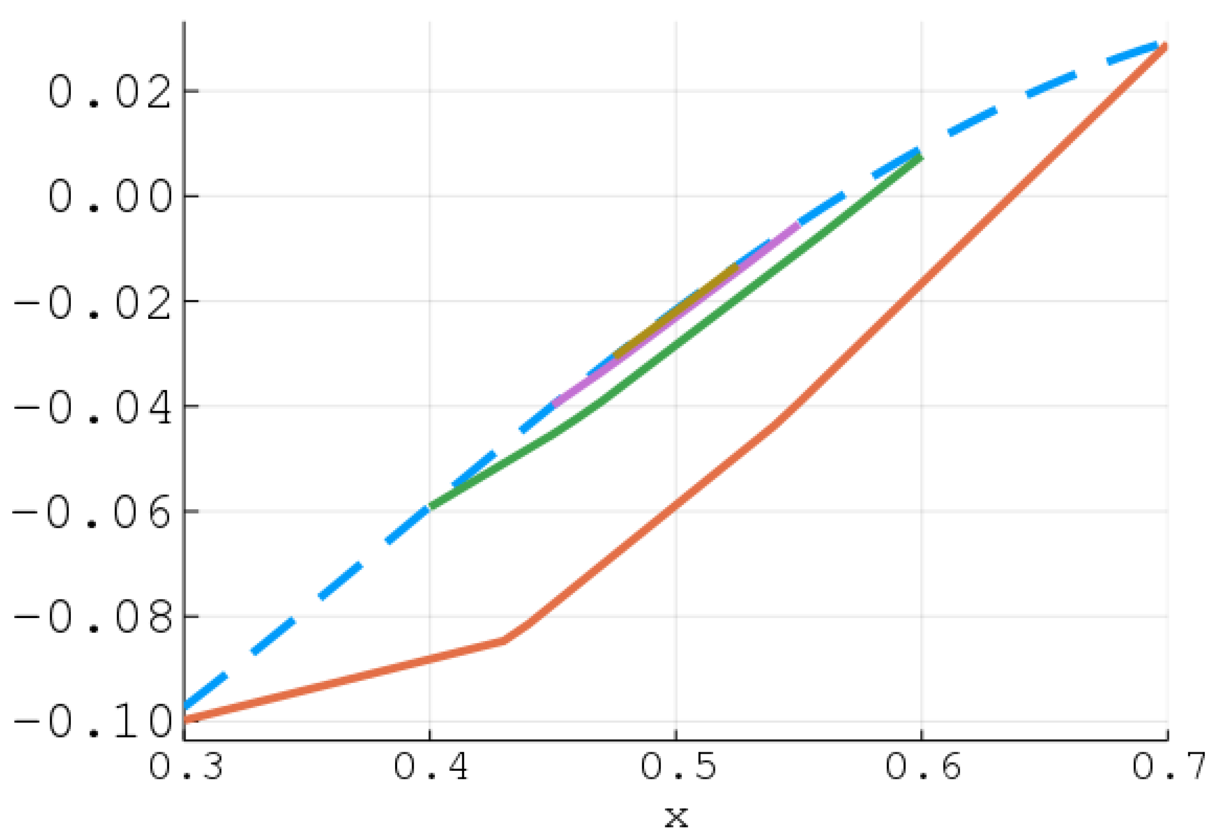
Example 1.

Consider sets $Z:=\mathbb{R}$ and $Q:=[-1,0]\subset Z$, a function $f:Z\to \mathbb{R}$ for which $f\left(z\right)\equiv z$, and a function $g:Z\to \mathbb{R}$ for which $g\left(z\right)\equiv z^2$. Consider the following schemes of convex estimators for f and g over all intervals $W\in \mathbb{I}Q$:

$${\underline{f}}_W^C\left(z\right)\equiv z,and{\underline{g}}_W^C\left(z\right)\equiv z^2-{\left(\mathrm{wid}W\right)}^2.$$

Observe that f and g are convex and smooth, as are their convex underestimators, and that Assumption 3 is satisfied. For each $ϵ\in [0,1]$, define $W_{ϵ}:=[-ϵ,0]\in \mathbb{I}Q$.

With these choices of functions and sets, it is readily verified that each $W_{ϵ}\in F$ and the NLP (2) is trivially solved on $W_{ϵ}$ for each $ϵ\in [0,1]$ to yield an optimal objective function value of

$$v\left(W_{ϵ}\right)=min\{z\in [-ϵ,0]:z^2\le 0\}=0,$$

with a minimum of $z^{*}:=0$ in each case.

Next, for each $ϵ\in [0,1]$, observe that

$${\underline{g}}_{W_{ϵ}}^C\left(z\right)\equiv z^2-{ϵ}^2,$$

and so the constraint ${\underline{g}}_{W_{ϵ}}^C\left(z\right)\le 0$ is satisfied for each $z\in W_{ϵ}$. Hence, the relaxed NLP (3) is trivially solved to yield:

$$\underline{v}\left(W_{ϵ}\right)=min\{z\in [-ϵ,0]:z^2-{ϵ}^2\le 0\}=\underset{z\in [-ϵ,0]}{min}z=-ϵ,$$

with a minimum of $z^{*}:=-ϵ$ in each case. So, for each $ϵ\in [0,1]$, we have

$$v\left(W_{ϵ}\right)-\underline{v}\left(W_{ϵ}\right)=ϵ=\mathrm{wid}{W}_{ϵ},$$

in which case

$$\underset{ϵ\to 0^{+}}{lim}\frac{v\left(W_{ϵ}\right)-\underline{v}\left(W_{ϵ}\right)}{{\left(\mathrm{wid}{W}_{ϵ}\right)}^2}=+\infty ,$$

and so the relaxed NLP (3) does not exhibit second-order pointwise convergence to (2).

The above example shows that nontrivial constraints may determine whether second-order pointwise convergence holds, even when schemes of convex underestimators for the objective and constraints are available with second-order pointwise convergence and even when the original NLP (2) is convex. This is essentially because, as in the above example, it is possible for a small perturbation of a nontrivial inequality constraint to change the corresponding feasible set significantly. In such cases, it is possible for the optimal objective function value of (3) to approach the optimal objective function value of (2) slowly as W shrinks, if at all. A nonconvexity of the components of $\mathbf{g}$ may present additional obstacles but is not the primary hindrance here.

A sufficient condition for the second-order pointwise convergence of (3) may, nevertheless, be obtained by strengthening Assumption 3 as follows. The extra requirements of this assumption are adopted from Shapiro [47], who used similar requirements to rule out pathological behavior in a perturbation analysis for NLPs. These requirements are essentially second-order sufficient conditions to ensure that the feasible set of (2) is somewhat stable under perturbations. Recall that no such additional assumptions were needed in the bound-constrained case explored in Theorem 2.

Assumption 4.

Suppose that Assumption 3 holds and that the functions f and $\mathbf{g}$ are twice-continuously differentiable on Z. For each $W\in F$, express the bound constraints in the NLPs (2) and (3) as explicit inequality constraints, and append these to $\mathbf{g}$. For each $W\in F$, let $M\left(W\right)\subset W$ denote the optimal solution set for the NLP (2), and suppose that all of the following conditions are satisfied for each $\mathbf{y}\in M\left(W\right)$.

1.

The NLP (2) satisfies the linear-independence constraint qualification (LICQ). That is, with $I\left(\mathbf{y}\right)$ denoting the subset of $\{1,\dots ,m\}$ for which $g_i\left(\mathbf{y}\right)=0$, the gradients $\nabla g_i\left(\mathbf{y}\right)$ for $i\in I\left(\mathbf{y}\right)$ are linearly independent. Hence, as shown by Rockafellar [46], there exist unique multipliers ${\mu }_i\left(W\right)\ge 0$ (depending on W but not $\mathbf{y}$) for each $i\in \{1,\dots ,m\}$ for which

• $0=\nabla f\left(\mathbf{y}\right)+{\sum }_{i=1}^m{\mu }_i\left(W\right)\nabla g_i\left(\mathbf{y}\right)$, and 
• ${\mu }_i\left(W\right)=0$ for each $i\notin I\left(\mathbf{y}\right)$.

2.

${\mu }_i\left(W\right)>0$ for each $i\in I\left(\mathbf{y}\right)$.

3.

Any vector $\mathbf{w}\in {\mathbb{R}}^n$ that satisfies both of the following conditions

• ${\mathbf{w}}^{\mathrm{T}}\nabla g_i\left(\mathbf{y}\right)=0$ for each $i\in I\left(\mathbf{y}\right)$, and 
• ${\mathbf{w}}^{\mathrm{T}}({\nabla }^{2}f\left(\mathbf{y}\right)+{\sum }_{i=1}^m{\mu }_i\left(W\right){\nabla }^2{g}_i\left(\mathbf{y}\right))\mathbf{w}=0$

is also an element of the linear space tangent to $M\left(W\right)$ at $\mathbf{y}$.

Theorem 3.

If Assumption 4 holds, then the relaxed NLP (3) exhibits second-order pointwise convergence to (2) over all $W\in F$, as does the LP (4) based on subgradient-cutting mappings.

Proof. 

Under Assumption 4, Theorem 2 shows that the LP (4) is, in each case, equivalent to an instance of (3) (adopting different schemes of underestimators that nevertheless still satisfy Assumption 4). Hence, it suffices to show only that the relaxed NLP (3) exhibits second-order pointwise convergence to (2).

By Assumption 4, there exists $\tau >0$ for which, for each $W\in F$,

$$\begin{array}{cc}\hfill 0& \le \underset{\mathbf{z}\in W}{sup}(f\left(\mathbf{z}\right)-{\underline{f}}_W^C\left(\mathbf{z}\right))\le \tau {\left(\mathrm{wid}W\right)}^2\hfill \\ \hfill \mathrm{and}0& \le \underset{\mathbf{z}\in W}{sup}(g_i\left(\mathbf{z}\right)-{\underline{g}}_{i,W}^C\left(\mathbf{z}\right))\le \tau {\left(\mathrm{wid}W\right)}^2,\forall i\in \{1,\dots ,m\}.\hfill \end{array}$$

For each $W\in F$, consider the following variants of the NLP (2):

$$\begin{array}{cc}\hfill \underset{\mathbf{z}\in W}{min}& f\left(\mathbf{z}\right)\hfill \\ \hfill \mathrm{s}.\mathrm{t}.& g\left(\mathbf{z}\right)-\tau {\left(\mathrm{wid}W\right)}^2\le 0,\forall i=\{1,\dots ,m\},\hfill \end{array}$$

(5)

and

$$\begin{array}{cc}\hfill \underset{\mathbf{z}\in W}{min}& {\underline{f}}_W^C\left(\mathbf{z}\right)\hfill \\ \hfill \mathrm{s}.\mathrm{t}.& g\left(\mathbf{z}\right)-\tau {\left(\mathrm{wid}W\right)}^2\le 0,\forall i=\{1,\dots ,m\},\hfill \end{array}$$

(6)

and let $v^{†}\left(W\right)$ and ${\underline{v}}^{†}\left(W\right)$ denote the respective optimal objective function values for (5) and (6). Analogously to the construction of $M\left(W\right)$, let $\underline{M}\left(W\right)$, $M^{†}\left(W\right)$, and ${\underline{M}}^{†}\left(W\right)$ denote the respective optimal solution sets for (3), (5), and (6); these and $M\left(W\right)$ are all nonempty compact sets. Choose the respective optimal solutions $\mathit{\xi }\left(W\right)\in M\left(W\right)$, $\underline{\mathit{\xi }}\left(W\right)\in \underline{M}\left(W\right)$, ${\mathit{\xi }}^{†}\left(W\right)\in M^{†}\left(W\right)$, and ${\underline{\mathit{\xi }}}^{†}\left(W\right)\in {\underline{M}}^{†}\left(W\right)$, so that the distance $\parallel \mathit{\xi }\left(W\right)-{\mathit{\xi }}^{†}\left(W\right)\parallel$ is minimized. (Such a choice is always possible due to Weierstrass’s Theorem and Lemma 1 in Section 5 of Filippov [48].) By comparing the feasible sets and objective functions of the constructed NLPs, observe that $v\left(W\right)\ge \underline{v}\left(W\right)\ge {\underline{v}}^{†}\left(W\right)$ for each $W\in F$. Hence, it suffices to establish the existence of ${\tau }_v>0$ for which, for each $W\in F$,

$$v\left(W\right)-{\underline{v}}^{†}\left(W\right)\le {\tau }_v{\left(\mathrm{wid}W\right)}^2.$$

Now, by construction of ${\mathit{\xi }}^{†}\left(W\right)$ and noting that (5) and (6) share the same feasible set, observe that $f\left({\mathit{\xi }}^{†}\left(W\right)\right)\le f\left({\underline{\mathit{\xi }}}^{†}\left(W\right)\right)$. Thus, for each $W\in F$,

$$v^{†}\left(W\right)-{\underline{v}}^{†}\left(W\right)=f\left({\mathbf{\xi }}^{†}\left(W\right)\right)-{\underline{f}}_W^C\left({\underline{\mathbf{\xi }}}^{†}\left(W\right)\right)\le f\left({\underline{\mathbf{\xi }}}^{†}\left(W\right)\right)-{\underline{f}}_W^C\left({\underline{\mathbf{\xi }}}^{†}\left(W\right)\right)\le \tau {\left(\mathrm{wid}W\right)}^2.$$

(7)

Next, under Assumption 4, observe that (2) satisfies the hypotheses of Corollary 3.2 by Shapiro [47]. Hence, M is “upper Lipschitzian” in the sense of [47]; since Q is compact, this implies the existence of ${\tau }_L>0$ (independent of W) for which

$$\parallel \mathbf{\xi }\left(W\right)-{\mathbf{\xi }}^{†}\left(W\right)\parallel \le {\tau }_L{\left(\mathrm{wid}W\right)}^2,\forall W\in F.$$

With $k_f$ denoting a Lipschitz constant for f on Q, it follows that, for each $W\in F$,

$$v\left(W\right)-v^{†}\left(W\right)=f\left(\mathbf{\xi }\left(W\right)\right)-f\left({\mathbf{\xi }}^{†}\left(W\right)\right)\le {\tau }_L{k}_f{\left(\mathrm{wid}W\right)}^2.$$

(8)

Adding Equations (7) and (8) yields

$$v\left(W\right)-{\underline{v}}^{†}\left(W\right)=(v\left(W\right)-v^{†}\left(W\right))+(v^{†}\left(W\right)-{\underline{v}}^{†}\left(W\right))\le (\tau +{\tau }_L{k}_f){\left(\mathrm{wid}W\right)}^2$$

for each $W\in F$, as required. ☐

To our knowledge, this is the first result establishing sufficient conditions for second-order pointwise convergence for relaxations of NLPs with nontrivial constraints. While Assumption 4 is somewhat stringent, it crucially does not require each optimal solution set $M\left(W\right)$ to be a singleton, as is typically assumed in quantitative sensitivity analyses for NLPs. Observe that the NLP considered in Example 1 does not satisfy the LICQ and, thus, does not satisfy Assumption 4.

The proof of Theorem 3 does not make use of the convexity of the relaxations ${\underline{f}}_W^C$ and ${\underline{g}}_{i,W}^C$ at all, beyond establishing the independence of the multipliers ${\mu }_i\left(W\right)$ to $\mathbf{y}$ in Assumption 4. It may be possible—though nontrivial—to exploit this convexity to weaken the hypotheses of Theorem 3.

While any equality constraint $h\left(\mathbf{z}\right)=0$ may be represented as the pair $\pm h\left(\mathbf{z}\right)\le 0$ of inequality constraints, this transformation yields an NLP that can never satisfy the LICQ and, thus, cannot satisfy Assumption 4. One way to extend Theorem 3 to NLPs with equality constraints without violating the LICQ is to relax each equality constraint $h\left(\mathbf{z}\right)=0$ by replacing it with two weaker inequality constraints:

$$h\left(\mathbf{z}\right)-ϵ\le 0\mathrm{and}-h\left(\mathbf{z}\right)-ϵ\le 0,$$

for small $ϵ>0$. Affine equality constraints may alternatively be eliminated by changing variables appropriately.

3.3. Constructing Subgradient-Cutting Mappings

Constructing subgradient-cutting mappings for functions or outer-approximating LPs (4) for NLPs in practice involves making several decisions; this section presents some suggestions for handling these decisions.

The simplest way to generate suitable points ${\mathit{\zeta }}_W\in {\mathbf{s}}_{\alpha }\left(W\right)$ is to choose ${\mathit{\zeta }}_W$ to be the midpoint of the interval W. This choice is valid regardless of $\alpha$ and is straightforward to compute.

The sets $B_W$ on which subgradients are evaluated may, in principle, be chosen in any manner; we suggest using points for which data is already available if possible or leveraging any prior knowledge concerning which points might be useful. In the absence of any such prior knowledge, Latin hypercube sampling (as described by Audet and Hare [49]) is a straightforward method for generating pseudo-random points that, in a sense, sample all of W. Intuitively, including more elements in $B_W$ results in a larger LP (4) and demands more subgradient evaluations to set up but also yields a tighter relaxation (4) of (2). We consider the effect of the number of linearization points in $B_W$ on several test problems in Section 5 below.

As described earlier, several established relaxation schemes may be used to construct schemes of underestimators ${\{{\underline{f}}_W^C\}}_{W\in \mathbb{I}Q}$ and ${\{{\underline{g}}_{i,W}^C\}}_{W\in \mathbb{I}Q}$ with second-order pointwise convergence. Subgradients may then be computed using standard automatic differentiation tools [50] when all functions involved are continuously differentiable; in this case, subgradients coincide with gradients. Otherwise, if nonsmooth relaxations are employed, then dedicated nonsmooth variants of automatic differentiation [30,51] may be applied to compute subgradients efficiently.

4. Comparison with Established Relaxation Methods

In this section, we compare the subtangent-based approach of this article with established outer approximation (OA) methods [40,41,42,52] and a recent subgradient-based enhancement of the McCormick relaxations by Najman and Mitsos [34].

OA approximates nonlinear convex relaxations as the pointwise maximum of the collection of their affine supports [42]. There are several established schemes for constructing the affine supports in OA, such as interval bisection, slope bisection, maximum error rules, and cord rules [42]. The convergence result of this paper applies to all of these schemes in principle, assuming that they are based on an underlying relaxation scheme with second-order pointwise convergence and that a subdomain’s midpoint is always chosen as one linear support. These complement the convergence results in References [37,42], which show that for any fixed subdomain, the piecewise-affine convex relaxations constructed by combining the linear supports converge quadratically to the dominating convex relaxations as the number of linearization points increases.

Najman and Mitsos [34] propose a tighter variant of McCormick relaxations of compositions of known intrinsic functions (which include the standard scientific calculator operations). This variant provides improved interval bounds for every composed function compared with classic McCormick relaxations and, thus, typically results in tighter overall relaxations for the composite function. The improved bounds are described by constructing simple affine or piecewise-affine relaxations for each factor and minimizing or maximizing these relaxations, resulting in tighter bounds. This process can be repeated based on the new bounds to get further tighter bounds of each factor. Then, tighter overall relaxations are approximated by their subtangents at midpoints of intervals. In the current article’s approach, on the other hand, the overall composite function is approximated by piecewise-affine relaxations; individual functions are not considered directly, and  there is no requirement to use McCormick relaxations. Both approaches can be combined; the tight relaxations of the Najman-Mitsos method may be employed as the underlying convex relaxations of which the subtangents are used in Theorem 2. Notably, the numerical results of Najman and Mitsos [34] suggest that it is not computationally worthwhile to select linearization points (such as the sets $B_W$ we consider), optimally using optimization solvers; based on this result, we do not recommend choosing the sets $B_W$ by solving a nontrivial optimization problem.

5. Implementation and Examples

This section discusses an implementation of the outer-approximating LPs (4), which was used to illustrate the convergence features discussed in this article.

5.1. Implementation in Julia

A numerical implementation in Julia v0.6.4 [39] was developed to solve nonconvex NLPs of the form (2) to global optimality, by using outer-approximating LPs of the form (4) to obtain lower bounds in an overarching branch-and-bound method for a deterministic global optimization. For simplicity, the central-scaling factor $\alpha$ is set to 0 in each case, so the midpoint of each interval W is always selected to be one of the linearization points at which the subgradients are evaluated. For each $i\in \{1,\dots ,m\}$, the sets $B_W^{\left(i\right)}$ are set to $B_W$. Equality constraints are effectively replaced in each case by a pair of inequality constraints; a satisfaction of Assumption 4 was not verified.

This implementation uses EAGO v0.1.2 [53,54] to carry out a simple branch-and-bound method (without any range reduction) and to compute convex relaxations of nonconvex functions. JuMP v0.18.2 [55] is used as an interface with optimization solvers; CPLEX v12.8 is used to solve LPs, and IPOPT v3.12.8 [56] is used to solve NLPs. Convex relaxations and subgradients are computed automatically in EAGO using either the standard McCormick relaxations [30,31] or the differentiable McCormick relaxations [38], combined with the interval-refining algorithm of Najman and Mitsos [34]. Latin hypercube sampling, as described by Audet and Hare [49], is adopted to select linearization points pseudo-randomly while sampling the entire subdomains in question. All numerical results presented in the following section were obtained by running this implementation on a Dell Precision T3400 workstation with a 2.83 GHz Intel Core2 Quad CPU. One core and 512 MB of memory were dedicated to each job.

5.2. Convergence Illustration

A first numerical example illustrates the second-order convergence results of this article.

Example 2.

As in Reference [38], consider the function

$$f:[0.3,0.7]\to \mathbb{R}:x\mapsto (x-x^2)(\log x-e^{-x}).$$

This function is plotted in Figure 1, along with a series of subgradient-cutting relaxations constructed as described in Definition 5. These relaxations were evaluated using the implementation described above on intervals of the form $X\left(ϵ\right):=[0.5-ϵ,0.5+ϵ]$, for each $ϵ:=0.4\left(2^{-k}\right)$, where $k\in \{1,\cdots ,20\}$.

With ${\varphi }_{X\left(ϵ\right)}$ denoting the relaxation of f constructed on $X\left(ϵ\right)$, Figure 2 presents a log-log plot of the maximum discrepancy ${sup}_{x\in X\left(ϵ\right)}(f\left(x\right)-{\varphi }_{X\left(ϵ\right)}\left(x\right))$ against the width of the interval $X\left(ϵ\right)$, together with a reference line with a slope of 2. The agreement between these two suggests that the convex relaxations ${\varphi }_{\mathbf{x}}\left(ϵ\right)$ exhibit second-order pointwise convergence to f as $ϵ\to 0^{+}$.

5.3. Optimization Test Problems

The described implementation was applied to three nonconvex NLP instances from the MINLPLib benchmark library [57], to examine the performance of LP outer approximations in a global optimization setting, and to consider the effect of including more linearization points in each set $B_W$. Small but relatively difficult nonconvex problems were chosen in each case. For comparison, these problems were also solved using the state-of-the-art global optimization solver BARON v18.5.8 [58,59] in GAMS. GAMS formulations for these problems were downloaded from the MINLPLib website [57] and were adapted to include bounds on any unbounded variables. These problems were considered to be solved to global optimality (by either our implementation or BARON) whenever the determined upper and lower bounds were equal to within either an absolute tolerance of ${10}^{-6}$ or a relative tolerance of ${10}^{-3}$. In each of these cases, our implementation (which does not employ range reduction) outperformed BARON with range reduction disabled; while not conclusive, this does suggest that piecewise-affine outer approximations of McCormick relaxations without auxiliary variables are competitive.

Example 3.

The first considered NLP instance wasbearing, which has 14 continuous variables, 10 equality constraints, and 3 inequality constraints, and is as follows.

$$\begin{array}{cccc}\underset{\mathbf{x}\in X,t\in \mathbb{R}}{min}\hfill & t\hfill & & \\ \mathrm{s}.\mathrm{t}.\hfill & \hfill & \hfill 10000t-10000x_7-10000x_8& =0\hfill \\ & \hfill & \hfill -1.42857142857143x_4{x}_6+10000x_8& =0\hfill \\ & \hfill & \hfill 10x_7{x}_9-0.00968946189201592x_3(x_1^4-x_2^4)& =0\hfill \\ & \hfill & \hfill 143.3076x_{10}{x}_4-10000x_7& =0\hfill \\ & \hfill & \hfill 3.1415927x_6{\left(0.001x_9\right)}^3-6e-6x_3{x}_4{x}_{13}& =0\hfill \\ & \hfill & \hfill 101000x_{12}{x}_{13}-1.57079635x_6{x}_{14}& =0\hfill \\ & \hfill & \hfill {\log }_{10}(0.8+8.112x_3)-10964781961.4318x_{11}^{-3.55}& =0\hfill \\ & \hfill & \hfill -0.5x_{10}+x_{11}& =560\hfill \\ & \hfill & \hfill x_1-x_2& \ge 0\hfill \\ & \hfill & \hfill 0.0307x_4^2-0.3864{\left(0.0062831854x_1{x}_9\right)}^2{x}_6& \le 0\hfill \\ & \hfill & \hfill 101000x_{12}-15707.9635x_{14}& \le 0\hfill \\ & \hfill & \hfill -(\ln \left(x_1\right)-\ln \left(x_2\right))+x_{13}& =0\hfill \\ & \hfill & \hfill -(x_1^2-x_2^2)+x_{14}& =0\hfill \end{array}$$

(9)

Since finite upper bounds of some decision variables were not provided in MINLPLib, we set them to reasonable values for branch-and-bound purposes. The considered domains for the variables $\mathbf{x}$ are shown in

Table 1. The considered domains of variables $\mathbf{x}$ when solving (9).

Component	Lower Bound	Upper Bound
$x_1$	1	6
$x_2$	1	6
$x_3$	1	6
$x_4$	1	6
$x_6$	990	1000
$x_7$	0.0001	2
$x_8$	0.0001	2
$x_9$	1	2
$x_{10}$	50	50
$x_{11}$	550	600
$x_{12}$	1	3
$x_{13}$	0.0001	3
$x_{14}$	0.001	10

.

Applying our implementation in EAGO with lower bounds computed using LP outer approximations Equation (4), this problem is solved to a global minimum of $t^{*}=1.931$.

Table 2. The impact of the number of linearization points $(1+|B_W\left|\right)$ on our implementation’s branch-and-bound solution time for (9).

# Linearization Points	Lower-Bounding Time (s) *	Upper-Bounding Time (s) *	Total Time (s) *	# Iterations *
1	73.94	654.10	733.47	15,309
2	17.39	93.66	111.84	2217
4	10.25	26.13	36.68	737
8	12.54	17.47	30.26	484
16	20.34	13.09	33.68	402
32	35.76	13.38	49.46	364
64	66.38	10.35	77.17	332

* Each number here is the average of 10 runs. The package loading time in Julia is excluded from the reported solving time.

shows the impact on solution time of the number of linearization points $(1+|B_W\left|\right)$ whose subgradients are used to construct the subgradient-cutting mappings. As described above, these were chosen pseudo-randomly using Latin hypercube sampling. Among the numbers of linearization points considered, 8 was time-optimal for this example; we expect this is because too few linearization points yields looser relaxations and poorer lower bounds early in the branch-and-bound process, whereas too many linearization points yields larger LP outer approximations (4) for lower bounding, requiring excessive computational time to solve. Our implementation was run both with and without the Najman–Mitsos interval-refining algorithm [34];

Table 3. The solution statistics for our implementation when applied to (9).

# lin. pts. †	N-M ‡	Lower-Bounding Time (s) *	Upper-Bounding Time (s) *	Total Time (s) *	# Iterations *
1	Yes	70.56	596.16	672.04	15,309
1	No	53.15	581.41	639.77	15,309
2	Yes	17.39	93.66	111.84	2217
2	No	16.96	125.41	140.77	2923
4	Yes	10.25	26.13	36.68	737
4	No	11.33	55.91	67.71	1194

* Each number here is the average of 10 runs. The package loading time in Julia is excluded from the reported solving time. ${}^{†}$ The number of linearization points $(1+|B_W\left|\right)$ at which subgradients were evaluated. ${}^{‡}$ “Yes” if Najman–Mitsos interval tightening was employed.

shows comparable solution times in each case.

This problem was also solved with BARON in GAMS, both with and without range reduction, with the results shown in

Table 4. The results of BARON v18.5.8 in GAMS when applied to (9), with 1000 s of solver time allocated in each case.

Range Reduction Used?	No	Yes
Wall clock time	1020.00	1030.00
Total CPU time	1000.00	1000.00
Total no. of BaR * iterations	282,404	467,659
Best solution found at node	184,858	1
Max. no. of nodes in memory	40,177	53,517
Best upper bound identified	1.95	1.91
Best lower bound identified	1.02	1.65

* Branch-and-reduce.

. (Our implementation did not incorporate range reduction.) No solution was identified before the allocated time of 1000 s in either case. We were unable to determine why; this did not appear to be an issue of setting tolerances incorrectly (such as constraint satisfaction tolerances), and the lower-bounding LP statistics were not readily available. Perhaps the highly nonlinear logarithmic terms interfere with BARON’s outer approximation methods in this case.

Example 4.

The second considered NLP instance from the MINLPLib library wasex6_2_11, with 4 continuous variables and 2 equality constraints and with bound constraints as provided by the library. This instance is shown below.    

$$\begin{array}{cc}\hfill \underset{\mathbf{x}\in X,t\in \mathbb{R}}{min}& t\hfill \\ \hfill \mathrm{s}.\mathrm{t}.& -\left(\right(15.3261663216011x_2+23.2043471859416x_3\hfill \\ & +6.69678129464404x_4)\ln (2.1055x_2+3.1878x_3+0.92x_4)\hfill \\ & +1.04055250396734x_2-2.24199441248417x_3+3.1618173099828x_4\hfill \\ & +6.4661663216011x_2\ln (x_2/(2.1055x_2+3.1878x_3+0.92x_4))\hfill \\ & +12.2043471859416x_3\ln (x_3/(2.1055x_2+3.1878x_3+0.92x_4))\hfill \\ & +0.696781294644034x_4\ln (x_4/(2.1055x_2+3.1878x_3+0.92x_4))\hfill \\ & +9.86x_2\ln (x_2/(1.972x_2+2.4x_3+1.4x_4))\hfill \\ & +12x_3\ln (x_3/(1.972x_2+2.4x_3+1.4x_4))\hfill \\ & +7x_4\ln (x_4/(1.972x_2+2.4x_3+1.4x_4))\hfill \\ & +(1.972x_2+2.4x_3+1.4x_4)\ln (1.972x_2+2.4x_3+1.4x_4)\hfill \\ & +1.972x_2\ln (x_2/(1.972x_2+0.283910843616504x_3+3.02002220174195x_4))\hfill \\ & +2.4x_3\ln (x_3/(1.45991339466884x_2+2.4x_3+0.415073537580851x_4))\hfill \\ & +1.4x_4\ln (x_4/(0.602183324335333x_2+0.115623371371275x_3+1.4x_4))\hfill \\ & -17.2981663216011x_2\ln \left(x_2\right)-25.6043471859416x_3\ln \left(x_3\right)\hfill \\ & -8.09678129464404x_4\ln \left(x_4\right))+t=0\hfill \\ & x_2+x_3+x_4=1\hfill \end{array}$$

(10)

Using our implementation, the problem is solved to a global minimum of $t^{*}=-2.67\times {10}^{-6}$.

Table 5. The solution statistics for our implementation when applied to (10).

# lin. pts. ${}^{†}$	N-M ${}^{‡}$	Lower-Bounding Time (s) *	Upper-Bounding Time (s) *	Total Time (s) *	# Iterations *
1	Yes	573.26	2356.06	3133.24	470,291
1	No	400.54	2028.58	2600.11	479,501
2	Yes	323.64	882.06	1278.40	210,928
2	No	360.95	1393.27	1872.82	310,279
4	Yes	251.70	513.98	806.21	136,107
4	No	322.95	1003.76	1404.62	245,125

* Each number here is the average of 5 runs. The package loading time in Julia is excluded from the reported solving time. ${}^{†}$ The number of linearization points $(1+|B_W\left|\right)$ at which subgradients were evaluated. ${}^{‡}$ “Yes” if Najman–Mitsos interval tightening was employed.

summarizes the results of our implementation, including the impact on solution time of the number of linearization points and the interval-computing algorithm. No range reduction was employed. This case study also suggests that using multiple linearization points can reduce the computational time required.

BARON could not solve this problem in 1000 s without range reduction, throwing an error suggesting the bounds were inappropriate, but did solve it with range reduction during preprocessing, obtaining the same optimal solution as our implementation. The corresponding statistics are displayed in

Table 6. The solution statistics for (10), using BARON with range reduction.

Wall clock time (s)	13.00
Total CPU time used (s)	12.48
Total no. of BaR * iterations	12,475
Max. no. of nodes in memory	357

* Branch-and-reduce.

.

Example 5.

The final considered NLP instance from the MINLPLib library wasprocess, shown as follows, with bound constraints as provided by the library.

$$\begin{array}{cccc}\underset{\mathbf{x}\in X,t\in \mathbb{R}}{min}\hfill & t\hfill & & \\ \mathrm{s}.\mathrm{t}.\hfill & \hfill & \hfill 5.04x_2+0.035x_3+3.36x_4+10x_9-0.063x_1{x}_8& =t\hfill \\ & \hfill & \hfill -3x_8+x_{10}& =-133\hfill \\ & \hfill & \hfill x_7+0.222x_{10}& =35.82\hfill \\ & \hfill & \hfill 1.22x_1-x_2-x_4& =0\hfill \\ & \hfill & \hfill -(x_3+x_4)/x_2+x_6& =0\hfill \\ & \hfill & \hfill -0.325x_5-1.098x_6+x_8+0.038x_6^2& =57.425\hfill \\ & \hfill & \hfill x_1-(0.13167x_6-0.00667x_6^2+1.12)x_2& =0\hfill \\ & \hfill & \hfill -0.001(x_1{x}_5{x}_7/(-x_5+98))+x_9& =0\hfill \end{array}$$

(11)

Our Julia implementation solves this problem to a global minimum of $t^{*}=-1161.34$; the solution statistics are listed in

Table 7. The solution statistics for our implementation applied to (11).

# lin. pts. ${}^{†}$	N-M ${}^{‡}$	Lower-Bounding Time (s) *	Upper-Bounding Time (s) *	Total Time (s) *	# Iterations *
1	Yes	10.06	33.71	45.69	4133
1	No	17.63	95.34	116.28	8939
2	Yes	7.20	13.32	21.67	2312
2	No	13.66	37.72	53.54	4662
4	Yes	6.87	7.65	15.45	1394
4	No	13.27	19.32	34.13	3044
8	Yes	8.39	5.13	14.28	1064
8	No	18.53	16.36	36.30	2769

* Each number here is the average of 10 runs. The package loading time in Julia is excluded from the reported solving time. ${}^{†}$ The number of linearization points $(1+|B_W\left|\right)$ at which subgradients were evaluated. ${}^{‡}$ “Yes” if Najman–Mitsos interval tightening was employed.

. Qualitatively, the results display similar trends to Example 3.

When range reduction was turned off in BARON, the upper and lower bounds did not converge by the end of the allocated 1000 s. (Recall that range reduction is not yet included in our implementation.) The best lower bound obtained by that time was $\overline{t}=-3085.43$. With range reduction, BARON solved the problem rapidly. The solution statistics for BARON are presented in

Table 8. The solution statistics for (11) using BARON, with 1000 s of solver time allocated in each case.

Range Reduction Used?	No	Yes
Wall clock time (s)	1002.00	1.00
Total CPU time (s)	1000.00	0.44
Total no. of BaR * iterations	330,033	563
Best solution found at node	298,558	9
Max. no. of nodes in memory	40,307	51
Best upper bound determined	−1161.34	−1161.34
Best lower bound determined	−3085.43	−1162.37

* Branch-and-reduce.

.

5.4. Application: Power Scheduling

A practical example from References [60,61] considers an application in electrical engineering, with two electrical generators connected to a net with three nodes. The constraints enforce that the power flowing into a node balances the power flowing out. The NLP formulation is shown below, and the lower/upper bounds of variables are provided in

Table 9. The bound constraints for decision variables in (12).

Component	Lower Bound	Upper Bound
$x_1$	0.5	1.2
$x_2$	0.5	1.2
$x_3$	0	0.3
$x_4$	0	0.3
$x_5$	0.90909	1.0909
$x_6$	0.90909	1.0909
$x_7$	0.90909	1.0909
$x_8$	$-0.5$	0.3
$x_9$	$-0.5$	0.3

.

$$\begin{array}{cc}\hfill \underset{\mathbf{x}\in X,t\in \mathbb{R}}{min}& t\hfill \\ \hfill \mathrm{s}.\mathrm{t}.& 0.4-x_1+2C{x}_5^2+x_5{x}_6(D\sin (-x_8)-C\cos (-x_8))+x_5{x}_7(D\sin (-x_9)-C\cos (-x_9))=0\hfill \\ & 0.4-x_2+2C{x}_6^2+x_5{x}_6(D\sin \left(x_8\right)-C\cos \left(x_8\right))+x_5{x}_7(D\sin (x_8-x_9)-C\cos (x_8-x_9))=0\hfill \\ & 0.2-x_3+2D{x}_5^2-x_5{x}_6(C\sin (-x_8)+D\cos (-x_8))-x_5{x}_7(C\sin (-x_9)+D\cos (-x_9))=0\hfill \\ & 0.2-x_4+2D{x}_6^2-x_5{x}_6(C\sin \left(x_8\right)+D\cos \left(x_8\right))-x_5{x}_7(C\sin (x_8-x_9)+D\cos (x_8-x_9))=0\hfill \\ & 0.8+2C{x}_7^2+x_5{x}_7(D\sin \left(x_9\right)-C\cos \left(x_9\right))+x_6{x}_7(D\sin (x_9-x_8)-C\cos (x_9-x_8))=0\hfill \\ & -0.337+2D{x}_7^2-x_5{x}_7(C\sin \left(x_9\right)+D\cos \left(x_9\right))-x_6{x}_7(C\sin (x_9-x_8)+D\cos (x_9-x_8))=0\hfill \\ & t\ge 3000x_1+1000x_1^3+2000x_2+666.667x_2^3\hfill \\ & C=(48.4/50.176)\sin \left(0.25\right)\hfill \\ & D=(48.4/50.176)\cos \left(0.25\right)\hfill \end{array}$$

(12)

This problem was solved with our implementation to a global minimum of $t^{*}=5055.0$, agreeing with a previously located local minimum [61] obtained using the local solvers CONOPT and MINOS (but not previously verified to be a global minimum). The global optimization solvers BARON and ANTIGONE [62] cannot be used to solve this problem as they do not support the trigonometric operations.

6. Conclusions and Future Work

This article shows that, under mild assumptions, if piecewise-affine convex relaxations of functions are constructed using subtangents of an original relaxation scheme, then the piecewise-affine relaxation scheme will inherit second-order pointwise convergence from the original scheme. A foundation for the second-order pointwise convergence of NLPs with nontrivial constraints is also provided, along with sufficient conditions motivated by Shapiro [47] for exhibiting this convergence. Combining these results, if outer-approximating LPs (4) are constructed from NLPs using subtangents, and the NLP-specific sufficient conditions for convergence are satisfied, then these LPs inherit second-order pointwise convergence. Ultimately, these results motivate using subtangents in practice: even though their use weakens a relaxation scheme, they do not weaken the scheme enough to introduce clustering into a branch-and-bound-style global optimization method when the developed sufficient conditions are satisfied. Moreover, their simplicity makes them easier to use in practice, as our implementation in Julia via EAGO demonstrates.

Future work will involve developing the Julia implementation further and further developing the convergence analysis for NLPs to better make use of convexity. Moreover, second-order pointwise convergence does not address a branch-and-bound method’s performance early on in the branch-and-bound tree; we expect that developing tighter convex relaxation schemes will still be beneficial to the performance of global optimization algorithms.

References

1. Li, M.; Mu, H.; Li, N.; Ma, B. Optimal design and operation strategy for integrated evaluation of CCHP (combined cooling heating and power) system. Energy 2016, 99, 202–220. [Google Scholar] [CrossRef]
2. Tan, Z.F.; Zhang, H.J.; Shi, Q.S.; Song, Y.H.; Ju, L.W. Multi-objective operation optimization and evaluation of large-scale NG distributed energy system driven by gas-steam combined cycle in China. Energy Build. 2014, 76, 572–587. [Google Scholar] [CrossRef]
3. Wang, J.J.; Jing, Y.X.; Zhang, C.F. Optimization of capacity and operation for CCHP system by genetic algorithm. Appl. Energy 2010, 87, 1325–1335. [Google Scholar] [CrossRef]
4. Vo, D.N.; Ongsakul, W. Improved merit order and augmented Lagrange Hopfield network for short term hydrothermal scheduling. Energy Convers. Manag. 2009, 50, 3015–3023. [Google Scholar] [CrossRef]
5. Nguyen, T.T.; Vo, D.N.; Dinh, B.H. An effectively adaptive selective cuckoo search algorithm for solving three complicated short-term hydrothermal scheduling problems. Energy 2018, 155, 930–956. [Google Scholar] [CrossRef]
6. Dai, Y.; Wang, J.; Gao, L. Parametric optimization and comparative study of Organic Rankine Cycle (ORC) for low grade waste heat recovery. Energy Convers. Manag. 2009, 50, 576–582. [Google Scholar] [CrossRef]
7. Yu, H.; Eason, J.; Biegler, L.T.; Feng, X. Simultaneous heat integration and techno-economic optimization of Organic Rankine Cycle (ORC) for multiple waste heat stream recovery. Energy 2017, 119, 322–333. [Google Scholar] [CrossRef]
8. Yang, H.; Lu, L.; Zhou, W. A novel optimization sizing model for hybrid soar-wind power generation system. Sol. Energy 2007, 81, 76–84. [Google Scholar] [CrossRef]
9. Mouret, S.; Grossmann, I.E.; Pestiaux, P. A novel priority-slot based continuous-time formulation for crude-oil scheduling problems. Ind. Eng. Chem. Res. 2009, 48, 8515–8528. [Google Scholar] [CrossRef]
10. Zavala-Río, A.; Femat, R.; Santiesteban-Cos, R. An analytical study on the logarithmic mean temperature difference. Rev. Mexicana Ingenierá Quḿica 2005, 4, 406–411. (In English) [Google Scholar]
11. Demissie, A.; Zhu, W.; Belachew, C.T. A multi-objective optimization model for gas pipeline operations. Comput. Chem. Eng. 2017, 100, 94–103. [Google Scholar] [CrossRef]
12. Glotić, A.; Glotić, A.; Kitak, P.; Pihler, J.; Tičar, I. Optimization of hydro energy storage plants by using differential evolution algorithm. Energy 2014, 77, 97–107. [Google Scholar] [CrossRef]
13. Lopez-Echeverry, J.S.; Reif-Acherman, S.; Araujo-Lopez, E. Peng-Robinson equation of state: 40 years through cubics. Fluid Phase Equilib. 2017, 447, 39–71. [Google Scholar] [CrossRef]
14. Najafi, H.; Najafi, B.; Hoseinpoori, P. Energy and cost optimization of a plate and fin heat exchanger using genetic algorithm. Appl. Therm. Eng. 2011, 31, 1839–1847. [Google Scholar] [CrossRef]
15. Rios, L.M.; Sahinidis, N.V. Derivative-free optimization: A review of algorithms and comparison of software implementations. J. Glob. Optim. 2013, 56, 1247–1293. [Google Scholar] [CrossRef]
16. Holland, J.H. Adaptation in Natural and Artificial Systems; The University of Michigan Press: Ann Arbor, MI, USA, 1975. [Google Scholar]
17. Storn, R.; Price, K. Differential evolution—A simple and efficient heuristic for global optimization over continuous spaces. J. Glob. Optim. 1997, 11, 341–359. [Google Scholar] [CrossRef]
18. Kennedy, J.; Eberhart, R. Particle swarm optimization. In Proceedings of the IEEE International Conference on Neural Networks, Piscataway, NJ, USA, 27 November–1 December 1995. [Google Scholar]
19. Gau, C.Y.; Stadtherr, M.A. Deterministic global optimization for error-in-variables parameter estimation. AIChE J. 2002, 48, 1192–1197. [Google Scholar] [CrossRef]
20. Vidigal, L.M.; Director, S.W. A design centering algorithm for nonconvex regions of acceptability. IEEE Trans. Comput.-Aided Des. Integr. Circuits Syst. 1982, 1, 13–24. [Google Scholar] [CrossRef]
21. Ghaohui, L.E.; Oks, M.; Oustry, F. Worst-case value-at-risk and robust portfolio optimization: A conic programming approach. Oper. Res. 2003, 51, 543–556. [Google Scholar] [CrossRef]
22. Paté-Cornell, M.E. Uncertainties in risk analysis: Six levels of treatment. Reliab. Eng. Syst. Saf. 1996, 54, 95–111. [Google Scholar] [CrossRef]
23. Huang, H.; Adjiman, C.S.; Shah, N. Quantitative framework for reliable safety analysis. AIChE J. 2002, 48, 78–96. [Google Scholar] [CrossRef]
24. Falk, J.E.; Soland, R.M. An algorithm for separable nonconvex programming problems. Manag. Sci. 1969, 15, 550–569. [Google Scholar] [CrossRef]
25. Du, K.; Kearfott, R.B. The cluster problem in multivariate global optimization. J. Glob. Optim. 1994, 5, 253–265. [Google Scholar] [CrossRef] [Green Version]
26. Bompadre, A.; Mitsos, A. Convergence rate of McCormick relaxations. J. Glob. Optim. 2012, 52, 1–28. [Google Scholar] [CrossRef]
27. Wechsung, A.; Schaber, S.D.; Barton, P.I. The cluster problem revisited. J. Glob. Optim. 2014, 58, 429–438. [Google Scholar] [CrossRef]
28. Adjiman, C.; Dallwig, S.; Floudas, C.; Neumaier, A. A global optimization method αBB, for general twice-differentiable constrained NLPs: I. Theoretical advances. Comput. Chem. Eng. 1998, 22, 1137–1158. [Google Scholar] [CrossRef]
29. Adjiman, C.; Androulakis, I.; Floudas, C. A global optimization method αBB, for general twice-differentiable constrained NLPs: II. Implementation and computational results. Comput. Chem. Eng. 1998, 22, 1159–1179. [Google Scholar] [CrossRef]
30. Mitsos, A.; Chachaut, B.; Barton, P.I. McCormick-based relaxations of algorithms. SIAM J. Optim. 2009, 20, 573–601. [Google Scholar] [CrossRef]
31. McCormick, G.P. Computability of global solutions to factorable nonconvex programs: Part I. Convex underestimating problems. Math. Program. 1976, 10, 147–175. [Google Scholar] [CrossRef]
32. Tsoukalas, A.; Mitsos, A. Multivariate McCormick relaxations. J. Glob. Optim. 2014, 59, 633–662. [Google Scholar] [CrossRef] [Green Version]
33. Scott, J.K.; Stuber, M.D.; Barton, P.I. Generalized McCormick relaxations. J. Glob. Optim. 2011, 51, 569–606. [Google Scholar] [CrossRef]
34. Najman, J.; Mitsos, A. Tighter McCormick relaxations through subgradient propagation. arXiv 2017, arXiv:1710.09188. [Google Scholar]
35. Najman, J.; Mitsos, A. Convergence Analysis of Multivariate McCormick Relaxations. J. Glob. Optim 2015, 66, 597–628. [Google Scholar] [CrossRef]
36. Khan, K.A. Subtangent-based approaches for dynamic set propagation. In Proceedings of the 57th IEEE Conference on Decision and Control, Miami Beach, FL, USA, 17 December 2018. [Google Scholar]
37. Rote, G. The convergence rate of the sandwich algorithm for approximating convex functions. Computing 1992, 48, 337–361. [Google Scholar] [CrossRef] [Green Version]
38. Khan, K.A.; Watson, H.A.J.; Barton, P.I. Differentiable McCormick relaxations. J. Glob. Optim. 2017, 67, 687–729. [Google Scholar] [CrossRef]
39. Bezanson, J.; Edelman, A.; Karpinski, S.; Shah, V.B. Julia: A Fresh Approach to Numerical Computing. SIAM Rev. 2017, 59, 65–98. [Google Scholar] [CrossRef] [Green Version]
40. Duran, M.A.; Grossmann, I.E. An outer-approximation algorithm for a class of mixed-integer nonlinear programs. Math. Program. 1986, 36, 307–339. [Google Scholar] [CrossRef]
41. Fletcher, R.; Leyffer, S. Solving mixed integer nonlinear programs by outer approximation. Math. Program. 1994, 66, 327–349. [Google Scholar] [CrossRef] [Green Version]
42. Tawarmalani, M.; Sahinidis, N.V. Global optimization of mixed-integer nonlinear programs: A theoretical and computational study. Math. Program. 2004, 99, 563–591. [Google Scholar] [CrossRef] [Green Version]
43. Stuber, M.D. A Differentiable Model for Optimizing Hybridization of Industrial Process Heat Systems with Concentrating Solar Thermal Power. Processes 2018, 6, 76. [Google Scholar] [CrossRef]
44. Horst, R.; Tuy, H. Global Optimization: Deterministic Approaches; Springer: Berlin, Germany, 1993. [Google Scholar]
45. Smith, M.B.; Pantelides, C.C. Global Optimisation of Nonconvex MINLPs. Comput. Chem. Eng. 1997, 21, S791–S796. [Google Scholar] [CrossRef]
46. Rockafellar, R.T. Convex Analysis; Princeton Landmarks in Mathematics Series; Princeton University Press: Princeton, NJ, USA, 1970. [Google Scholar]
47. Shapiro, A. Perturbation theory of nonlinear programs when the set of optimal solution is not a singleton. Appl. Math. Optim. 1988, 18, 215–229. [Google Scholar] [CrossRef]
48. Filippov, A.F. Differential Equations with Discontinuous Righthand Sides; Kluwer Academic Publishers: Dordrecht, The Netherlands, 1988. [Google Scholar]
49. Audet, C.; Hare, W. Derivative-Free and Blackbox Optimization; Springer Series in Operations Research and Financial Engineering; Springer International Publishing: Berlin/Heidelberg, Germany, 2017. [Google Scholar]
50. Griewank, A.; Walther, A. Evaluating Derivatives: Principles and Techniques of Algorithmic Differentiation, 2nd ed.; Other Titles in Applied Mathematics; SIAM: Philadelphia, PA, USA, 2008. [Google Scholar]
51. Beckers, M.; Mosenkis, V.; Naumann, U. Adjoint mode computation of subgradients for McCormick relaxations. In Recent Advances in Algorithmic Differentiation; Forth, S., Hovland, P., Phipps, E., Utke, J., Walther, A., Eds.; Springer: Berlin, Germany, 2012; pp. 103–113. [Google Scholar]
52. Tawarmalani, M.; Sahinidis, N.V. A polyhedral branch-and-cut approach to global optimization. Math. Program. 2005, 103, 225–249. [Google Scholar] [CrossRef]
53. Wilhelm, M.; Stuber, M.D. Easy Advanced Global Optimization (EAGO): An Open-Source Platform for Robust and Global Optimization in Julia. In Proceedings of the AIChE Annual Meeting 2017 Minneapolis, Minneopolis, MN, USA, 31 October 2017. [Google Scholar]
54. Wilhelm, M.; Stuber, M.D. EAGO: Easy Advanced Global Optimization Julia Package. Available online: https//github.com/PSORLab/EAGO.jl (accessed on 1 May 2018).
55. Dunning, I.; Huchette, J.; Lubin, M. JuMP: A Modeling Language for Mathematical Optimization. SIAM Rev. 2017, 59, 295–320. [Google Scholar] [CrossRef] [Green Version]
56. Wächter, A.; Biegler, L.T. On the implementation of an interior-point filter line-search algorithm for large-scale nonlinear programming. Math. Program. 2006, 106, 25–57. [Google Scholar] [CrossRef]
57. MINLPLib: A Library of Mixed-Integer and Continuous Nonlinear Programming Instances. 2019. Available online: http://www.minlplib.org/instances.html (accessed on 1 March 2019).
58. Ryoo, H.S.; Sahinidis, N.V. A branch-and-reduce approach to global optimization. J. Glob. Optim. 1996, 8, 107–138. [Google Scholar] [CrossRef]
59. Sahinidis, N.V. BARON: A general purpose global optimization software package. J. Glob. Optim. 1996, 8, 201–205. [Google Scholar] [CrossRef]
60. Hock, W.; Schittkowski, K. Test Examples for Nonlinear Programming Codes; Lecture Notes in Economics and Mathematical Systems; Springer: Berlin/Heidelberg, Germany, 1981. [Google Scholar]
61. Andrei, N. Nonlinear Optimization Applications Using the GAMS Technology; Springer Optimization and Its Applications; Springer: New York, NY, USA, 2013. [Google Scholar]
62. Misener, R.; Floudas, C.A. ANTIGONE: Algorithms for Continuous/Integer Global Optimization of Nonlinear Equations. J. Glob. Optim. 2014, 59, 503–526. [Google Scholar] [CrossRef]
Figure 1. A plot of the function f in Example 1 (dashed) and its associated subgradient-cutting relaxations (solid) on intervals of the form [ 0.5 ϵ , 0.5 + ϵ ] for 0 < ϵ < 0.2 .
Processes 07 00221 g001
Figure 2. A log-log plot of d f : = sup x X ( ϵ ) ( f ( x ) ϕ X ( ϵ ) ( x ) ) vs. w : = 2 ϵ (circles) and a reference line (dotted) with a slope of 2, for Example 1.
Processes 07 00221 g002