Sensor Fault-Tolerant Control Design for Mini Motion Package Electro-Hydraulic Actuator

Abstract

With the rapid development of computer science and information and communication technology (ICT), increasingly intelligent, and complex systems have been applied to industries as well as human life. Fault-tolerant control (FTC) has, therefore, become one of the most important topics attracting attention from both engineers and researchers to maintain system performances when faults occur. The ultimate goal of this study was to develop a sensor fault-tolerant control (SFTC) to enhance the robust position tracking control of a class of electro-hydraulic actuators called mini motion packages (MMPs), which are widely used for applications requiring large force-displacement ratios. First, a mathematical model of the MMP system is presented, which is then applied in the position control process of the MMP system. Here, a well-known proportional, integrated and derivative (PID) control algorithm is employed to ensure the positional response to the reference position. Second, an unknown input observer (UIO) is designed to estimate the state vector and sensor faults using a linear matrix inequality (LMI) optimization algorithm. Then an SFTC is used to deal with sensor faults of the MMP system. The SFTC is formed of the fault detection and the fault compensation with the goal of determining the location, time of occurrence, and magnitude of the faults in the fault signal compensation process. Finally, numerical simulations were run to demonstrate the superior performance of the proposed approach compared to traditional tracking control.

1. Introduction

In modern industries, valve-driven hydraulic actuators (VHAs) have been used extensively due to their advantageous features such as simplicity and high-precision control for linear as well as nonlinear systems [1,2,3,4]. However, these actuators have some limitations, including low energy efficiency due to leakage through the valve of the hydraulic pump, and throttle losses. Electric motor-pump-driven hydraulic actuators, tagged as electro-hydraulic actuators (EHAs), have been recently introduced as an alternative to provide high output power at great energy efficiency [5,6]. A representative configuration of an EHA is depicted in Figure 1. Here, the position of the hydraulic cylinder is adjusted directly by the bidirectional pump, with the support of two pilot-operated check valves and two pressure relief valves [5,6]. Because of their advantages, various types of EHAs have been commercialized and are widely used in different industrial applications, including active vibration isolation of machine tools [7] and wing control and landing gear control in aircraft [8,9,10]. Among these, a class of compact EHAs from Kayaba Industrial Company, known as mini motion packages (MMPs), is considered one of the most feasible solutions for applications requiring short operating ranges and high output power.

However, when working in a disturbed environment, system nonlinearities with large uncertainties become critical challenges in utilizing EHAs to obtain high-precision positioning (or force) tracking control. The traditional linear control approaches derived for VHAs are therefore not suitable for this type of application due to the large control error [11], and the nonlinear schemes for EHA tracking control have attracted considerable attention from researchers and engineers to solve faults or failures of EHAs. Faults or failures arise from components of the EHA system such as failures in the electrical machine of the pump, the leakage faults of the pump and cylinder, aging and cable break faults of the sensor, and the others as polluted oil, etc. To address this issue, the fault-tolerant control (FTC) technique for EHAs was introduced. This technique handles the impacts of actuator faults (AFs) and sensor faults (SFs) [12,13,14,15,16,17,18], and sensor fault-tolerant control (SFTC) techniques are also used to solve the problems of SFs [19,20]. With the rapid development of mechatronics technology, increasingly intelligent and complex systems using the FTC technique have been applied to both industries and human life. Applications with EHAs also face new control challenges to maintain the system stability when a fault or failure occurs. In general, FTC is a complex combination of three major research fields, fault detection and isolation (FDI), robust control, and reconfigurable control. The FDI and the reconfigurable controller need to be robust against uncertainties and disturbances as in [21,22]. By using FTC techniques, the system still works as normal instead of stopping under the impacts of AFs and SFs [12,13,14,15,16,17,18]. Thus, the FTC plays a key role to improve the performance of systems prone to faults or failures. However, actuator failures cannot be handled [21]. In recent decades, various fault detection and diagnosis (FDD) and FTC techniques have been developed by researchers, such as the FDD schemes that use an extended Kalman filter (EKF) algorithm for isolating either the SF or the AF of the system [14,20,23]. In [23], the author applies FDI based on multiple hybrid Kalman filters to detect the fault process. Furthermore, the FTC technique in [14] utilizes Kalman filter reconfiguration, which helps ignore the feedback signal from the sensor when a sensor fault occurs. Especially in the FTC function [20], if a sensor fault appears, the feedback signal is formed from the estimation state of an unknown input observer (UIO). In contrast, this feedback signal will be the data transferred directly from the sensor. The systems described in these articles perform fault detection and isolation without removing the faults.

However, a recently developed FTC compensation technique removes the faults that come from the SFs or the AFs [19]. This technique has been successfully designed and applied in linear and nonlinear systems and is attracting several researchers. The two main tasks of this technology are to determine the estimated fault and to perform fault compensation. To obtain the estimated fault, some advanced observer methods are proposed, such as the sliding mode observer [15,24], the augmented observer [12,16,17,18,25,26,27,28], and sensor fault reconstruction [29,30]. In particular, a UIO of the system variable reconstruction has the benefits of not only estimating the state vector, but also the fault estimation, as shown in [18,29,30]. The estimations of the state and the fault are implemented by the augmented observer, based on a UIO of the system variable reconstruction and an LMI optimization algorithm. This method has advantages in the AF estimation and the SF estimation are performed by an LMI optimization algorithm so that the UIO to be asymptotically stable [29]. However, in [18], decoupling the unknown input disturbance created difficulty in practical applications. Therefore, the SFTC technology developed in this paper is based on a combination of the error calculation method described in [18] and the UIO of the system variable reconstruction with the LMI optimization algorithm given in [31]. We can clearly see the effects of using FTC technique compared with traditional tracking control in [31,32].

In this paper, an advanced SFTC technology is proposed for robust position tracking control of an MMP system under fault conditions. The classic PID control algorithm is employed to enhance the system tracking performance. First, the mathematical model of the MMP system is developed to simplify the control process of the EHA system, which is different from the methods in [5,6]. Second, a UIO is built from robust, observer-based reconstruction for the linear and nonlinear discrete-time system with an unknown input disturbance and SF. Here, the state estimation and the fault estimation are applied to the UIO of the system variable reconstruction, which is different from the approaches in [28,29,30]. Lyapunov’s stability condition and an LMI optimization algorithm are utilized for the asymptotical stability of the proposed state observer. Then an SFTC compensation technique is designed for the MMP system. According to this technique, the magnitude of the compensation signals is received from the fault estimation process of the UIO. The fault compensation decision is made based on the residual signal. Finally, numerical simulations are run to demonstrate the superior performance of the proposed approach compared with traditional tracking control.

The important contributions of this paper are summarized as follows:

• The piston position equation of the MMP system is established using the derivative of the dynamic system. This equation is transformed in the form of the nonlinear system or the nonlinear discrete-time system in state space. The main task of this step is to simplify the piston position control process of the MMP model. Additionally, the new control equations of the valves are successfully applied to the position control using the PID controller.
• To achieve asymptotic stability of the state observer, the UIO utilizing the optimization algorithm (LMI) for the linear and nonlinear discrete-time system is proposed. Our approach is described and validated by Lyapunov’s stability based on the error conditions. Finally, the matrix inequality is obtained to apply the LMI optimization algorithm.

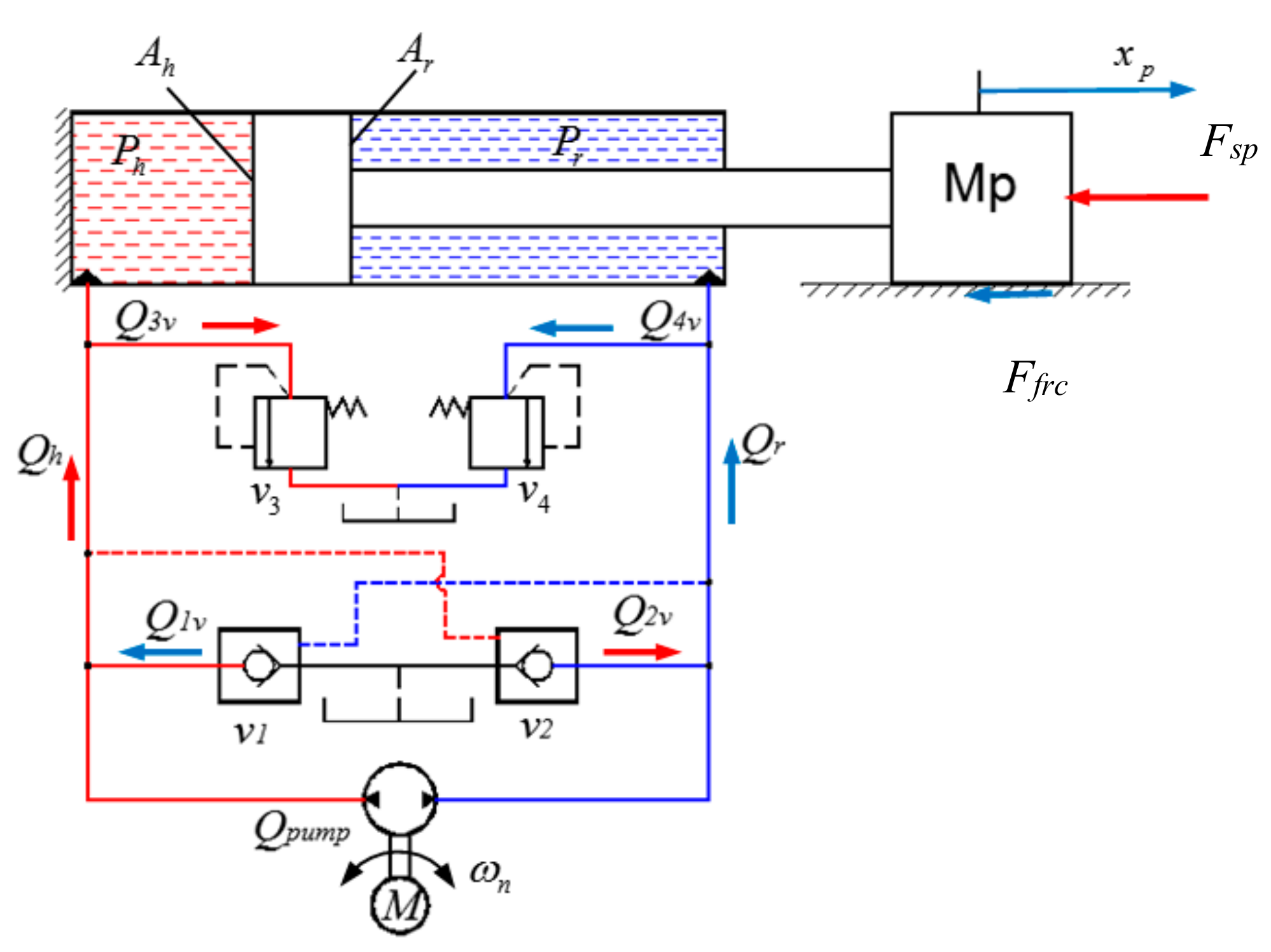
This paper is organized as follows. In Section 2, a mathematical model of the MMP system is addressed to simplify the control process of the EHA system and the numerical simulation process. In Section 3, a UIO-based sensor fault estimation using a reconstruction approach for systems is implemented, and necessary and sufficient conditions for the existence of a robust UIO are provided. LMI techniques are described for the discrete-time Lipschitz nonlinear systems. In Section 4, simulations with the MMP model using the proposed FTC technique are carried out and the results are discussed. Final conclusions are drawn in Section 5.

2. EHA Model

Referencing the schematic of the EHA system shown in Figure 1, the dynamics of the piston position can be written as [20]:

$$m_p{\ddot{x}}_p+B_v{\dot{x}}_p+F_{sp}+F_{frc}+d=A_h{P}_h-A_r{P}_r$$

(1)

where $m_p$ is the equivalent mass of the object M_p, $x_p$ is the piston position, ${\ddot{x}}_p$ and ${\dot{x}}_p$ are the acceleration and piston velocity, respectively, $P_h$ and $P_r$ are the pressure in two chambers, respectively, $A_h$ and $A_r$ are the piston area in two chambers, respectively, $F_{sp}$ is the external load force on the cylinder, d is the disturbance, $B_v$ is the viscosity damping coefficient, and $F_{frc}$ is the friction force.

The spring force $F_{sp}$ can be computed as:

$$F_{sp}=K_{sp}{x}_p$$

(2)

where $K_{sp}$ is stiffness of the spring.

The friction force $F_{frc}$ can be presented as [33]:

$$F_{frc}=\sqrt{2e}\left(F_{brk}-F_C\right)e^{-{\left(\frac{v_p}{v_{st}}\right)}^2}\hspace{0.17em}\frac{v_p}{v_{st}}+F_C\hspace{0.17em}\tanh \left(\frac{v_p}{v_{st}}\right)$$

(3)

where $F_{brk}$ and $F_C$ are breakaway friction and Coulomb friction, respectively. $v_p$, $v_{st}$, and $B_v$ are position velocity, Stribeck velocity threshold, and viscous friction coefficient, respectively.

The hydraulic continuity equations of the EHA system can be expressed as [5]:

$${\dot{P}}_h={\Delta }_1\left(Q_h-Q_i-{\dot{x}}_p{A}_h\right)$$

(4)

$${\dot{P}}_r={\Delta }_2\left(Q_r+Q_i+{\dot{x}}_p{A}_r\right)$$

(5)

where

$${\Delta }_1={\beta }_e/\left(V_{ch}+x_p{A}_h\right); {\Delta }_2={\beta }_e/\left(V_{cr}-x_p{A}_r\right); Q_{13i}=Q_{1v}-Q_{3v}-Q_i \mathrm{and} Q_{24i}=Q_{2v}-Q_{4v}+Q_i.$$

${\beta }_e$ is the effective bulk modulus in each chamber, and $V_{ch}$, and $V_{cr}$ are the initial control volumes of the two chambers.

The internal leakage flow rate of the cylinder $Q_i$ is described as [5]:

$$Q_i=C_{leak}(P_h-P_r)$$

(6)

where $C_{leak}$ is the coefficient of the internal leakage of the cylinder.

The flow rates into the two chambers of the cylinder are computed as [5]:

$$Q_h=Q_{pump}+Q_{1v}-Q_{3v}$$

(7)

$$Q_r=-Q_{pump}+Q_{2v}-Q_{4v}$$

(8)

where $Q_{1v}$ and $Q_{2v}$ are the flow rate through of the pilot-operated check valve on the left, and the pilot-operated check valve on the right, respectively. $Q_{3v}$ and $Q_{4v}$ are the flow rate through the pressure relief valve on the left and the pressure relief valve on the right in Figure 1.

The pump flow rate $Q_{pump}$ can be presented as [5]:

$$Q_{pump}=D_p\omega$$

(9)

where $D_p$ is displacement of the pump, and $\omega$ is the speed of the servo pump system.

The left pilot-operated check valve ($v_1$) is described as [34]:

$$Q_{1v}=C_d\hspace{0.17em}{A}_{1p}\sqrt{\frac{2}{\rho }}\frac{p_1}{{\left(p_1^2+P_{crack}^2\right)}^{1/4}}$$

(10)

where

$$A_{1p}=\{\begin{array}{ll}{A}_{leak}& if\hspace{0.17em}\hspace{0.17em}{p}_{1e}<p_{crack}\\ A_{leak}+k·(p_{1e}-p_{crack})& if\hspace{0.17em}\hspace{0.17em}{p}_{crack}<p_{1e}<p_{\max }\hspace{0.17em}\\ A_{\max }& if\hspace{0.17em}\hspace{0.17em}{p}_{1e}\ge p_{\max }\end{array},$$

$$p_{1e}=k_{pv}{P}_r-P_h;k=\frac{A_{\max }-A_{leak}}{p_{\max }-p_{crack}};p_1=-P_h.$$

P_crack, P_max, are the valve cracking pressure and the pressure needed to fully open the valve, respectively. A_pmax and A_leak, are the maximum valve opening area and the closed valve leakage area, respectively. C_d and K_pc are the valve coefficient and valve constant, respectively.

Similarly, the right pilot-operated check valve $\left(v_2\right)$ can be calculated as (10).

The flow rate through the pressure relief valve $\left(v_3\right)$ is determined according to the following Equations [34]:

$$Q_{3v}=C_{dp}\hspace{0.17em}{A}_{3p}\sqrt{\frac{2}{\rho }}\frac{p_3}{{\left(p_3^2+P_{3cr}^2\right)}^{1/4}}$$

(11)

where

$$A_{3p}=\{\begin{array}{ll}{A}_{leak}& if\hspace{0.17em}\hspace{0.17em}{p}_3<p_{set}\\ A_{leak}+k·(p_3-p_{set})& if\hspace{0.17em}{p}_{set}<p_3<p_{\max }\hspace{0.17em}\\ A_{\max }& if\hspace{0.17em}\hspace{0.17em}{p}_3\ge p_{\max }\end{array},$$

$$k=\left(A_{\max }-A_{leak}\right)/p_{reg};p_3=P_h.$$

The minimum pressure for turbulent flow $p_{3cr}$ is calculated according to the transition from a laminar to a turbulent regime, as defined by the following equation:

$$p_{3cr}=\left(P_3/2+P_{atm}\right)\left(1-B_{lam}\right),$$

where $P_{atm}$, and $B_{lam}$ are the atmospheric pressure and the pressure ratio at the transition between the laminar and turbulent regimes, respectively.

Similarly, the pressure relief valve $\left(v_4\right)$ can be calculated as (11).

Moreover, taking the derivative of (1) leads to:

$$m_p{\stackrel{⃛}{x}}_p+\mathrm{\Theta }{\ddot{x}}_p+K_{sp}{\dot{x}}_p+\mathrm{\Gamma }{\ddot{x}}_p=A_h{\dot{P}}_h-A_r{\dot{P}}_r$$

(12)

where

$$\mathrm{\Theta }=B_v+F_C/v_{cl}$$

$$\mathrm{\Gamma }=-\frac{F_C}{v_{cl}}\tanh {\left(\frac{{\dot{x}}_p}{v_{cl}}\right)}^2+\frac{\sqrt{2e}\left(F_{brk}-F_C\right)e^{-{\left(\frac{{\dot{x}}_p}{v_{st}}\right)}^2}}{v_{st}^{}}-\frac{2\sqrt{2e}{\dot{x}}_p^2\left(F_{brk}-F_C\right)e^{-{\left(\frac{{\dot{x}}_p}{v_{st}}\right)}^2}}{v_{st}^3}.$$

Substituting (4) and (5) into (12), we obtain:

$$\begin{array}{ll}{m}_p{\stackrel{⃛}{x}}_p+\mathrm{\Theta }{\ddot{x}}_p+K_{sp}{\dot{x}}_p+\mathrm{\Gamma }{\ddot{x}}_p& =A_h{\dot{P}}_h-A_r{\dot{P}}_r\\ & =\left(A_h{\Delta }_1+A_r{\Delta }_2\right)\hspace{0.17em}{Q}_{pump}\hspace{0.17em}-\left(A_h^2{\Delta }_1+A_r^2{\Delta }_2\right){\dot{x}}_p+\mathrm{\Omega }\end{array}$$

(13)

where

$$\mathrm{\Omega }=A_h{\Delta }_1{Q}_{13i}-A_r{\Delta }_2{Q}_{24i}.$$

Finally, (13) can be rewritten as:

$${\stackrel{⃛}{x}}_p=-{\gamma }_1{\ddot{x}}_p-{\gamma }_2{\dot{x}}_p+g\left(x,u\right)$$

(14)

where

$$g\left(x,u\right)=-\left(\mathrm{\Gamma }/m_p\right){\ddot{x}}_p+\mathrm{\Omega }/m_p+{\gamma }_{4}u-{\gamma }_3{\dot{x}}_p\hspace{0.17em}$$

$${\gamma }_1=\mathrm{\Theta }/m_p;\hspace{0.17em}\hspace{0.17em}{\gamma }_2=K_{sp}/m_p;\hspace{0.17em}u=\omega .$$

Equation (14) can be built in form as:

$$\dot{x}=Ax+f(x,u)$$

(15)

where

$$\{\begin{array}{l}{x}_1=x_p;\\ {\dot{x}}_1=x_2={\dot{x}}_p;\\ {\dot{x}}_2=x_3={\ddot{x}}_p\\ {\dot{x}}_3=-{\gamma }_1{x}_3-{\gamma }_2{x}_2+g\left(x,u\right)\end{array};x={\left[\begin{array}{ccc}{x}_1^T& x_2^T& x_3^T\end{array}\right]}^T\mathrm{and}f(x,u)={\left[\begin{array}{ccc}0& 0& g^T(x,u)\end{array}\right]}^T.$$

The matrix A shown in (15) is the constant matrix. It can be expressed in a nonlinear discrete-time state space model as:

$$x_{k+1}=A_k{x}_k+{\varphi }_{x_k,u_k}$$

(16)

where

$$x_k={\left[\begin{array}{ccc}{x}_1^T(k)& x_2^T(k)& x_3^T(k)\end{array}\right]}^T$$

$$A_k=\left[\begin{array}{ccc}1& T_s& 0\\ 0& 1& T_s\\ 0& -T_s{\gamma }_2& \left(1-T_s{\gamma }_1\right)\end{array}\right],\mathrm{and}{\varphi }_{x_k,u_k}=\left[\begin{array}{c}0\\ 0\\ T_{s}g(x_k,u_k)\end{array}\right].$$

3. UIO-Based Reconstruction Approach

3.1. UIO for Linear Discrete-time System

A dynamics system with uncertainty is utilized in a linear discrete form with an additive unknown disturbance term as the following equation [18]:

$$\{\begin{array}{l}{x}_{k+1}=A_k{x}_k+B_k{u}_k+D_d{d}_k\\ \hspace{0.17em}{y}_k\hspace{0.17em}\hspace{0.17em}=C_k{x}_k+F_s{s}_k\end{array}$$

(17)

where $x_k\in {ℝ}^n$ is the state vector, $y_k\in {ℝ}^p$ is the outputs vector and $d_k\in {ℝ}^{r_d}$ is the unknown input or disturbance vector, and $s_k\in {ℝ}^q$ is the sensor fault. $A_k,B_k,C_k,D_d$, and $F_s$ are known constant matrices with suitable dimensions.

The system variable reconstruction of (17) can be rewritten in the following form:

$$\{\begin{array}{l}\overline{E}{\overline{x}}_{k+1}={\overline{A}}_k{\overline{x}}_k+{\overline{B}}_k{u}_k+\overline{G}{s}_k+{\overline{D}}_d{d}_k\\ \hspace{0.17em}\hspace{0.17em}\hspace{0.17em}\hspace{0.17em}\hspace{0.17em}\hspace{0.17em}{y}_k\hspace{0.17em}={\overline{C}}_k{\overline{x}}_k\end{array}$$

(18)

where

$$\begin{array}{c}\hspace{0.17em}\hspace{0.17em}{\overline{A}}_k=\left[\begin{array}{cc}{A}_k& 0\\ 0& -I_p\end{array}\right];\overline{E}=\left[\begin{array}{cc}{I}_n& 0\\ 0& 0_p\end{array}\right];{\overline{B}}_k={\left[\begin{array}{cc}{B}_k^T& 0_p^T\end{array}\right]}^T;\\ {\overline{C}}_k=\left[\begin{array}{cc}{C}_k& F_s\end{array}\right];{\overline{D}}_d=\left[\begin{array}{c}{D}_d\\ 0\end{array}\right];\overline{G}=\left[\begin{array}{c}0\\ I_p\end{array}\right];{\overline{x}}_k=\left[\begin{array}{c}{x}_k^{}\\ s_k\end{array}\right]\in {ℝ}^{\overline{n}}\end{array}$$

with $\overline{n}=n+p$.

Based on [18], the UIO model can be built by the influences of unknown inputs in the system (18) as:

$$\{\begin{array}{l}{\overline{z}}_{k+1}=F{\overline{z}}_k+\mathrm{\Sigma }{\overline{B}}_k{u}_k+L{y}_k\\ {\widehat{\overline{x}}}_k={\overline{z}}_k+H{y}_k\\ {\widehat{y}}_k={\overline{C}}_k{\widehat{\overline{x}}}_k\end{array}$$

(19)

where ${\widehat{\overline{x}}}_k\in {ℝ}^{\overline{n}}$, ${\widehat{y}}_k\in {ℝ}^p$, and ${\overline{z}}_k\in {ℝ}^{\overline{n}}$ are state vector estimation of ${\overline{x}}_k$, measurement output estimation vector and state vector of the observer, respectively. The observer matrices $F\in {ℝ}^{\overline{n}\times \overline{n}}$, $\mathrm{\Sigma }\in {ℝ}^{\overline{n}\times \overline{n}}$, $H\in {ℝ}^{\overline{n}\times p}$, $L\in {ℝ}^{\overline{n}\times p}$, $L_1\in {ℝ}^{\overline{n}\times p}$, and $L_2\in {ℝ}^{\overline{n}\times p}$ should be designed according to the state estimation error vector.

Similarly, by using [18], the estimation error can be defined as:

$${\overline{e}}_k={\overline{x}}_k-{\widehat{\overline{x}}}_k$$

(20)

and

$$\begin{array}{l}{\overline{e}}_{k+1}={\overline{x}}_{k+1}-{\widehat{\overline{x}}}_{k+1}\\ \hspace{0.17em}\hspace{0.17em}\hspace{0.17em}\hspace{0.17em}\hspace{0.17em}\hspace{0.17em}\hspace{0.17em}\hspace{0.17em}=\left(I_{\overline{n}}-H{\overline{C}}_k\right){\overline{x}}_{k+1}-{\overline{z}}_{k+1}\\ \hspace{0.17em}\hspace{0.17em}\hspace{0.17em}\hspace{0.17em}\hspace{0.17em}\hspace{0.17em}\hspace{0.17em}\hspace{0.17em}=\mathrm{\Sigma }{\overline{x}}_{k+1}-{\overline{z}}_{k+1}\end{array}$$

(21)

where

$$\mathrm{\Sigma }=I_{\overline{n}}-H{\overline{C}}_k$$

Multiplying both sides of the matrix Equation (18) by the matrix $\mathrm{\Sigma }$, Equation (18) can be rewritten as:

$$\mathrm{\Sigma }\overline{E}{\overline{x}}_{k+1}=\mathrm{\Sigma }{\overline{A}}_k{\overline{x}}_k+\mathrm{\Sigma }{\overline{B}}_k{u}_k\hspace{0.17em}\hspace{0.17em}+\mathrm{\Sigma }\overline{G}{s}_k+\mathrm{\Sigma }{\overline{D}}_d{d}_k$$

(22)

and from (19), we obtain

$$\begin{array}{ll}{\widehat{\overline{x}}}_{k+1}& =F{\overline{z}}_k+\mathrm{\Sigma }{\overline{B}}_k{u}_k+L{y}_k+H{\overline{C}}_k{\overline{x}}_{k+1}\\ & =F{\widehat{\overline{x}}}_k-FH{y}_k+\mathrm{\Sigma }{\overline{B}}_k{u}_k+L{y}_k+H{\overline{C}}_k{\overline{x}}_{k+1}\\ & =F{\widehat{\overline{x}}}_k-\left(FH-L_2\right)y_k+\mathrm{\Sigma }{\overline{B}}_k{u}_k+L_1{\overline{C}}_k{\overline{x}}_k+H{\overline{C}}_k{\overline{x}}_{k+1}\end{array}$$

(23)

where $L=L_1+L_2$

Using (20)–(23), we have:

$${\overline{e}}_{k+1}=F{\overline{e}}_k+\left[I_{\overline{n}}-\left(\mathrm{\Sigma }\overline{E}+H{\overline{C}}_k\right)\right]{\overline{x}}_{k+1}+\left[\left(\mathrm{\Sigma }{\overline{A}}_k\hspace{0.17em}-L_1{\overline{C}}_k\right)-F\right]{\overline{x}}_k+\left(FH-L_2\right)y_k+\mathrm{\Sigma }\overline{G}{s}_k+\mathrm{\Sigma }{\overline{D}}_d{d}_k$$

(24)

From (20), (21), and (24), the estimation error (25) can be represented as:

$${\overline{e}}_{k+1}=F{\overline{e}}_k+\mathrm{\Sigma }{\overline{D}}_d{d}_k$$

(25)

If the following conditions are satisfied

$$\begin{array}{r}\mathrm{\Sigma }\overline{E}+H{\overline{C}}_k=I_{\overline{n}}\\ \mathrm{\Sigma }\overline{G}=0\\ \mathrm{\Sigma }{\overline{A}}_k-L_1{\overline{C}}_k=F\\ FH=L_2\end{array}\}$$

(26)

without loss of generality, the matrix Σ can be defined:

$$\mathrm{\Sigma }=\left[\begin{array}{cc}{I}_n& {\delta }_1\\ -C_k& {\delta }_2\end{array}\right]$$

(27)

where ${\delta }_1\in {ℝ}^{nxp}$ and ${\delta }_2\in {ℝ}^{pxp}$ are arbitrary matrices.

By solving (26) and (27), we obtain:

$$\mathrm{\Sigma }=\left[\begin{array}{cc}{I}_n& 0\\ -C_k& 0\end{array}\right];\hspace{0.17em}{\delta }_1={\delta }_2=0;H=\left[\begin{array}{c}0\\ I_p\end{array}\right]$$

(28)

Lemma 1.

[18] The necessary and sufficient conditions for the existence of UIO (19), if the system (18) guarantees as follows:

$$\begin{array}{c}rank(C_k{D}_d)=rank(D_d)\\ \mathrm{a})\left[\begin{array}{cc}{A}_k-I_n& D_d\\ C_k& 0\end{array}\right]=n+r_d,\mathit{and}{D}_d\mathit{is}a\mathit{full}\mathit{column}\mathit{rank}\\ \mathrm{b})\left[\begin{array}{cc}{A}_k-z{I}_n& D_d\\ C_k& 0\end{array}\right]=n+r_d\forall z\mathit{with}\left|z\right|>1.\end{array}$$

Lemma 2.

[29] For the equation in the following form:

$$\dot{\zeta }\left(t\right)=\mathrm{\Phi }\zeta \left(t\right)+\mathsf{\Upsilon }u\left(t\right)$$

(29)

The eigenvalues of a given matrix $\mathrm{\Phi }\in {ℝ}^{n\times n}$ belong to the circular region $D\left(\alpha ,\rho \right)$ with the center α + j0 and the radius $\rho$ if and only if there exists a symmetric positive definite matrix $P\in {ℝ}^{n\times n}$ such that the following condition holds:

$$\left[\begin{array}{cc}-P& P\left(\mathrm{\Phi }-\alpha I_n\right)\\ *& -{\rho }^{2}P\end{array}\right]<0$$

(30)

Theorem 1.

For system (18), there exists a robust UIO in the form of (19) such that$\Vert e_{yk}\Vert \le \gamma \Vert d_k\Vert$, and a prescribed circular region$D\left(\alpha ,r\right)$, if there exists a positive-definite symmetric matrix$P_L\in {ℝ}^{\overline{n}\times \overline{n}}$and matrix$Q_L\in {ℝ}^{\overline{n}\times p}$, and a scalar$\gamma >0$such that the following inequalities hold:

$$\left[\begin{array}{cccc}-P_L& 0& {\left(\mathrm{\Sigma }{\overline{A}}_k\right)}_{}^T{P}_L-{\overline{C}}_k^T{Q}_L^T& {\overline{C}}_k^T\\ *& -\gamma I_d& {\left(\mathrm{\Sigma }{\overline{D}}_d\right)}^T{P}_L& 0\\ *& *& -P_L& 0\\ *& *& *& -\gamma I_P\end{array}\right]<0$$

(31)

and

$$\left[\begin{array}{cc}-P_L& P_L\mathrm{\Sigma }{\overline{A}}_k-Q_L{\overline{C}}_k-\alpha P_L\\ \ast & -r^2{P}_L\end{array}\right]<0\hspace{0.17em}$$

(32)

where$Q_L=P_L{L}_1$and output estimation error$e_{yk}^{}={\overline{C}}_k{\overline{e}}_k$

Then the state observer (18) is asymptotically stable.

Proof of (31).

Consider Lyapunov functions as $V_k={\overline{e}}_k^T{P}_L{\overline{e}}_k$; then its difference between two adjacent steps $\Delta V_k=V_{k+1}-V_k$ is given as:

$$\begin{array}{ll}\Delta V_k& =V_{k+1}-V_k\\ & ={\overline{e}}_{k+1}^T{P}_L{\overline{e}}_{k+1}-{\overline{e}}_k^T{P}_L{\overline{e}}_k\\ & ={\overline{e}}_k^T{F}^T{P}_{L}F{\overline{e}}_k+{\overline{e}}_k^T{F}^T{P}_L\mathrm{\Sigma }{\overline{D}}_d{d}_k-e_k^T{P}_L{e}_k+d_k^T{\left(\mathrm{\Sigma }{\overline{D}}_d\right)}^T{P}_{L}F{\overline{e}}_k\hspace{0.17em}+d_k^T{\left(\mathrm{\Sigma }{\overline{D}}_d\right)}^T{P}_L\mathrm{\Sigma }{\overline{D}}_d{d}_k\end{array}$$

(33)

or

$$\Delta V_k={\left[\begin{array}{c}{\overline{e}}_k\\ d_k\end{array}\right]}^T\left[\begin{array}{cc}{F}^T{P}_{L}F-P_L& F^T{P}_L\mathrm{\Sigma }{\overline{D}}_d\\ *& {\left(\mathrm{\Sigma }{\overline{D}}_d\right)}^T{P}_L\mathrm{\Sigma }{\overline{D}}_d\end{array}\right]\left[\begin{array}{c}{\overline{e}}_k\\ d_k\end{array}\right].$$

Based on the initial condition $\Vert e_{yk}\Vert \le \gamma \Vert d_k\Vert$, the matrix J in (34) can be presented as:

$$J={\left[\begin{array}{c}{\overline{e}}_k\\ d_k\end{array}\right]}^T\left[\begin{array}{cc}\frac{1}{\gamma }{\overline{C}}_k^T{\overline{C}}_k& 0\\ 0& -\gamma I_d\end{array}\right]\left[\begin{array}{c}{\overline{e}}_k\\ d_k\end{array}\right]\le 0$$

(34)

where $e_{yk}^{}={\overline{C}}_k{\overline{e}}_k$ is output estimation error.

From (33) and (34), the matrix $\mathsf{\Upsilon }$ can be expressed in the stable condition of system as:

$$\mathsf{\Upsilon }=\Delta V_k+J\le 0$$

(35)

Thus, (35) can be rewritten as:

$$\begin{array}{ll}\mathsf{\Upsilon }& ={\left[\begin{array}{c}{\overline{e}}_k\\ d_k\end{array}\right]}^T\left[\begin{array}{cc}{F}^T{P}_{L}F-P_L+\frac{1}{\gamma }{\overline{C}}_k^T{\overline{C}}_k& F^T{P}_L\mathrm{\Sigma }{\overline{D}}_d\\ *& {\left(\mathrm{\Sigma }{\overline{D}}_d\right)}^T{P}_L\mathrm{\Sigma }{\overline{D}}_d-\gamma I_d\end{array}\right]\left[\begin{array}{c}{\overline{e}}_k\\ d_k\end{array}\right]\\ & ={\chi }^T\mathrm{\Pi }\chi \end{array}$$

(36)

where

$$\chi ={\left[\begin{array}{cc}{\overline{e}}_k^T& d_k^T\end{array}\right]}^T$$

$$\mathrm{\Pi }=\left[\begin{array}{cc}-P_L+\frac{1}{\gamma }{\overline{C}}_k^T{\overline{C}}_k& 0\\ 0& -\gamma I_d\end{array}\right]+\left[\begin{array}{cc}{F}^T{P}_{L}F& F^T{P}_L\mathrm{\Sigma }{\overline{D}}_d\\ *& {\left(\mathrm{\Sigma }{\overline{D}}_d\right)}^T{P}_L\mathrm{\Sigma }{\overline{D}}_d\end{array}\right].$$

Using the Schur lemma [34] for the inequality (35) with $\mathrm{\Pi }<0$, then (31) is satisfied, once existent $J<0$ satisfies the condition $\Vert e_{yk}\Vert \le \gamma \Vert d_k^{}\Vert$. □

Proof of (32).

Applying (25) to Lemma 2, then (32) is satisfied. □

Although the linear UIO is developed here, there are still some limitations:

• Performance of the control system using the linear UIO can be inaccurate because of any unknown nonlinear terms.
• In fact, an MMP system is a nonlinear system with unknown nonlinearities and uncertainties [5,6].

To address this challenge, the nonlinear UIO is proposed and developed in the following section.

3.2. UIO for Nonlinear Discrete-time System

We consider the following nonlinear discrete-time system subject to an unknown input in the following form:

$$\{\begin{array}{l}{x}_{k+1}=A_k{x}_k+B_k{u}_k+{\varphi }_{x_k,u_k}+D_d{d}_k\\ \hspace{0.17em}y{\hspace{0.17em}}_k\hspace{0.17em}=C_k{x}_k+F_s{s}_k\end{array}$$

(37)

where ${\varphi }_{x_k,u_k}=\varphi \left(x_k,u_k\right)$ is a nonlinear function vector $\forall x_k,x_k\in {ℝ}^n,u_k\in {ℝ}^m$.

Based on [29], a Lipschitz constraint of the discrete-time nonlinear function vector ${\varphi }_{x_k,u_k}$ can be expressed as

$$\Vert \Delta {\varphi }_{x_k,u_k}\Vert \le \zeta \Vert e_k\Vert$$

(38)

where $\Vert \Delta {\varphi }_{x_k,u_k}\Vert =\Vert {\varphi }_{x_k,u_k}-{\varphi }_{{\widehat{x}}_k,u_k}\Vert$ and $\Vert e_k\Vert =\Vert x_k-{\widehat{x}}_k\Vert$.

Similar to (18), the system variable reconstruction for the nonlinear discrete-time system (37) is rewritten as:

$$\{\begin{array}{l}\overline{E}{\overline{x}}_{k+1}={\overline{A}}_k{\overline{x}}_k+{\overline{B}}_k{u}_k+{\overline{\varphi }}_{x_k,u_k}+\overline{G}{s}_k+{\overline{D}}_d{d}_k\\ \hspace{0.17em}{y}_k\hspace{0.17em}={\overline{C}}_k{\overline{x}}_k\end{array}$$

(39)

where ${\overline{\varphi }}_{x_k,u_k}={\left[\begin{array}{cc}{\varphi }_{x_k,u_k}& 0\end{array}\right]}^T\in {ℝ}^{\overline{n}}$.

From (38), we obtain

$$\Vert \Delta {\overline{\varphi }}_{x_k,u_k}\Vert \le \overline{\zeta }\Vert {\overline{e}}_k\Vert$$

(40)

where

$$\begin{array}{c} \Delta {\overline{\varphi }}_{x_k,u_k}={\overline{\varphi }}_{x_k,u_k}-{\overline{\varphi }}_{{\widehat{x}}_k,u_k}\\ {\overline{e}}_k={\overline{x}}_k-{\widehat{\overline{x}}}_k;\hspace{0.17em}\hspace{0.17em}\overline{\zeta }=\left[\begin{array}{cc}\zeta I_n& 0\\ 0& 0_p\end{array}\right]\in {ℝ}^{\overline{n}}\end{array}.$$

The UIO is built for the nonlinear discrete-time systems (38) as:

$$\{\begin{array}{l}{\overline{z}}_{k+1}=F_n{\overline{z}}_k+\mathrm{\Sigma }{\overline{B}}_k{u}_k+L{y}_k\hspace{0.17em}+\mathrm{\Sigma }{\overline{\varphi }}_{{\widehat{x}}_k,u_k}\\ {\widehat{\overline{x}}}_k={\overline{z}}_k+H{y}_k\end{array}$$

(41)

where vector $\mathrm{\Sigma }$ and $H$ are matrices to be designed for satisfying (28).

Furthermore, the estimation error is also computed following (20) and (21). It is easy to write (42) as:

$${\overline{e}}_{k+1}=F_n{\overline{e}}_k+\mathrm{\Sigma }\Delta {\overline{\varphi }}_{x_k,u_k}+\mathrm{\Sigma }{\overline{D}}_d{d}_k$$

(42)

if the following conditions are satisfied:

$$\begin{array}{r}\mathrm{\Sigma }\overline{E}+H{\overline{C}}_k=I_{\overline{n}}\\ \mathrm{\Sigma }\overline{G}=0\\ \mathrm{\Sigma }{\overline{A}}_k-L_1{\overline{C}}_k=F_n\\ F_{n}H=L_2\end{array}\}$$

(43)

The matrix Λ in the inequality condition (44) can be inferred from (40) as:

$$\mathrm{\Lambda }={\left[\begin{array}{c}{\overline{e}}_k\\ \Delta {\overline{\varphi }}_{x_k,u_k}\end{array}\right]}^T\left[\begin{array}{cc}-{\overline{\zeta }}^T\overline{\zeta }& 0\\ 0& I_{\overline{n}}\end{array}\right]\left[\begin{array}{c}{\overline{e}}_k\\ \Delta {\overline{\varphi }}_{x_k,u_k}\end{array}\right]\le 0$$

(44)

Theorem 2.

For system (39), there exists a robust UIO in the form of (41) such that the output estimation error satisfies$\Vert e_{yk}\Vert \le \mu \Vert d_k^{}\Vert$and a prescribed circular region$D\left(\alpha ,r\right)$if there exists a positive-definite symmetric matrix$P_n\in {ℝ}^{\overline{n}\times \overline{n}}$, matrix$Q_n\in {ℝ}^{\overline{n}\times p}$, and positive scalars$\mu ,$and$\epsilon$such that the following inequalities (41, 42) hold:

$$\left[\begin{array}{ccccc}-P_n+\epsilon {\overline{\zeta }}_{}^T\overline{\zeta }& 0& 0& {\left(\mathrm{\Sigma }{\overline{A}}_k\right)}_{}^T{P}_n-{\overline{C}}_k^T{Q}_n^T& {\overline{C}}_k^T\\ *& -\epsilon I_{\overline{n}}& 0& {\mathrm{\Sigma }}^T{P}_n& 0\\ *& *& -\mu I_d& {\left(\mathrm{\Sigma }{\overline{D}}_d\right)}^T{P}_n& 0\\ *& *& *& -P_n& 0\\ *& *& *& *& -\mu I_p\end{array}\right]<0$$

(45)

and

$$\left[\begin{array}{cc}-P_n& P_n\mathrm{\Sigma }{\overline{A}}_k-Q_n{\overline{C}}_k-\alpha P_n\\ \ast & -r^2{P}_n\end{array}\right]<0$$

(46)

Then the state observer (41) is asymptotically stable.

Proof of (45).

Consider a Lyapunov function as $V_k={\overline{e}}_k^T{P}_n{\overline{e}}_k$; then its difference between two adjacent steps $\Delta V_k=V_{k+1}-V_k$ is given as:

$$\begin{array}{ll}\Delta V_k& =V_{k+1}-V_k\\ & ={\overline{e}}_{k+1}^T{P}_n{\overline{e}}_{k+1}-{\overline{e}}_k^T{P}_n{\overline{e}}_k\\ & ={\lambda }^T\left[\begin{array}{ccc}{F}_n^T{P}_n{F}_n-P_n& F_n^T{P}_n\mathrm{\Sigma }& F_n^T{P}_n\mathrm{\Sigma }{\overline{D}}_d\\ *& {\mathrm{\Sigma }}^T{P}_n\mathrm{\Sigma }& {\mathrm{\Sigma }}^T{P}_n\mathrm{\Sigma }{\overline{D}}_d\\ *& *& {\left(\mathrm{\Sigma }{\overline{D}}_d\right)}^T{P}_n\mathrm{\Sigma }{\overline{D}}_d\end{array}\right]\lambda \end{array}$$

(47)

where

$$\lambda ={\left[\begin{array}{ccc}{\overline{e}}_k^T& \Delta {\overline{\varphi }}_{x_k,u_k}^T& d_k^T\end{array}\right]}^T.$$

Moreover, (44) can be described as:

$$\mathrm{\Lambda }={\lambda }^T\left[\begin{array}{ccc}-{\overline{\zeta }}^T\overline{\zeta }& 0& 0\\ 0& I_{\overline{n}}& 0\\ 0& 0& 0\end{array}\right]\lambda \le 0$$

(48)

Combining (47) and (48) leads to:

$$\begin{array}{ll}\Delta V_k& \le {\lambda }^T\left[\begin{array}{ccc}{F}_n^T{P}_n{F}_n-P_n& F_n^T{P}_n\mathrm{\Sigma }& F_n^T{P}_n\mathrm{\Sigma }{\overline{D}}_d\\ *& {\mathrm{\Sigma }}^T{P}_n\mathrm{\Sigma }& {\mathrm{\Sigma }}^T{P}_n\mathrm{\Sigma }{\overline{D}}_d\\ *& *& {\left(\mathrm{\Sigma }{\overline{D}}_d\right)}^T{P}_n\mathrm{\Sigma }{\overline{D}}_d\end{array}\right]\lambda -\epsilon \mathrm{\Lambda }\\ & ={\lambda }^T\left[\begin{array}{ccc}{F}_n^T{P}_n{F}_n-P_n+\epsilon {\overline{\zeta }}^T\overline{\zeta }& F_n^T{P}_n\mathrm{\Sigma }& F_n^T{P}_n\mathrm{\Sigma }{\overline{D}}_d\\ *& {\mathrm{\Sigma }}^T{P}_n\mathrm{\Sigma }-\epsilon I_{\overline{n}}& {\mathrm{\Sigma }}^T{P}_n\mathrm{\Sigma }{\overline{D}}_d\\ *& *& {\left(\mathrm{\Sigma }{\overline{D}}_d\right)}^T{P}_n\mathrm{\Sigma }{\overline{D}}_d\end{array}\right]\lambda \end{array}$$

(49)

Based on the measurement error condition $\Vert e_{yk}\Vert \le \mu \Vert d_k\Vert$ of the output, the matrix $J_n$ in (50) can be presented as:

$$J_n={\left[\begin{array}{c}{\overline{e}}_k\\ d_k\end{array}\right]}^T\left[\begin{array}{cc}\frac{1}{\mu }{\overline{C}}_k^T{\overline{C}}_k& 0\\ 0& -\mu I_d\end{array}\right]\left[\begin{array}{c}{\overline{e}}_k\\ d_k\end{array}\right]\le 0$$

(50)

A matrix $T_n$ is defined as:

$$T_n=\Delta V_k+J_n$$

(51)

Equation (52) can be described using (49) and (51) as:

$$\begin{array}{ll}{T}_n& \le {\lambda }^T\left[\begin{array}{ccc}{F}_n^T{P}_n{F}_n-P_n+\epsilon {\overline{\zeta }}^T\overline{\zeta }+\frac{1}{\mu }{\overline{C}}_k^T{\overline{C}}_k& F_n^T{P}_n\mathrm{\Sigma }& F_n^T{P}_n\mathrm{\Sigma }{\overline{D}}_d\\ *& {\mathrm{\Sigma }}^T{P}_n\mathrm{\Sigma }-\epsilon I_{\overline{n}}& {\mathrm{\Sigma }}^T{P}_n\mathrm{\Sigma }{\overline{D}}_d\\ *& *& {\left(\mathrm{\Sigma }{\overline{D}}_d\right)}^T{P}_n\mathrm{\Sigma }{\overline{D}}_d-\mu I_d\end{array}\right]\lambda \\ & ={\lambda }^T{\mathrm{\Pi }}_n\lambda \end{array}$$

(52)

where

$${\mathrm{\Pi }}_n=\left[\begin{array}{ccc}{F}_n^T{P}_n{F}_n^{}& F_n^T{P}_n\mathrm{\Sigma }& F_n^T{P}_n\mathrm{\Sigma }{\overline{D}}_d\\ *& {\mathrm{\Sigma }}^T{P}_n\mathrm{\Sigma }& {\mathrm{\Sigma }}^T{P}_n\mathrm{\Sigma }{\overline{D}}_d\\ *& *& {\left(\mathrm{\Sigma }{\overline{D}}_d\right)}^T{P}_n\mathrm{\Sigma }{\overline{D}}_d\end{array}\right]+\left[\begin{array}{ccc}-P_n+\epsilon {\overline{\zeta }}^T\overline{\zeta }+\frac{1}{\mu }{\overline{C}}_k^T{\overline{C}}_k& 0& 0\\ *& -\epsilon I_{\overline{n}}& 0\\ *& *& -\mu I_d\end{array}\right]$$

(53)

Appling the Schur lemma [33] to (51) with ${\mathrm{\Pi }}_n<0$, we obtain:

$${\mathrm{\Pi }}_{n^{\prime }}=\left[\begin{array}{cccc}-P_n+\epsilon {\overline{\zeta }}_{}^T\overline{\zeta }+\frac{1}{\mu }{\overline{C}}_k^T{\overline{C}}_k& 0& 0& {\left(\mathrm{\Sigma }{\overline{A}}_k\right)}_{}^T{P}_n-{\overline{C}}_k^T{Q}_n^T\\ *& -\epsilon I_{\overline{n}}& 0& {\mathrm{\Sigma }}^T{P}_n\\ *& *& -\mu I_d& {\left(\mathrm{\Sigma }{\overline{D}}_d\right)}^T{P}_n\\ *& *& *& -P_n\end{array}\right]$$

(54)

Similarly, applying the Schur complement lemma [33] to (54) with ${\mathrm{\Pi }}_{n^{\prime }}<0$, then the inequality (45) is satisfied once $J_n<0$ satisfies the condition $\Vert e_{yk}\Vert \le \mu \Vert d_k^{}\Vert$. □

Proof of (46).

Applying (41) to Lemma 2, then (46) is satisfied. □

In summary, the design procedure for this fault estimator is implemented in the following steps:

• Step 1: Construct the augmented system (39) for the discrete-time system (37).
• Step 2: Determine the matrices $Q_n$, $P_n$, and $L_1=P_n^{-1}{Q}_n$ to solve the LMI defined by the matrix inequality (45, 46).
• Step 3: Calculate the gain matrices $F_n$, $L_2$ and $L$ using (46).
• Step 4: Obtain the state and fault estimation as ${\widehat{x}}_k^{}=\left[\begin{array}{cc}{I}_n& o_{n\times r}\end{array}\right]{\widehat{\overline{x}}}_k^{}$, and ${\widehat{s}}_k={\overline{C}}_s{\widehat{\overline{x}}}_k$, respectively,

where ${\overline{C}}_s=\left[\begin{array}{cc}{o}_{r\times n}& I_r\end{array}\right]$.

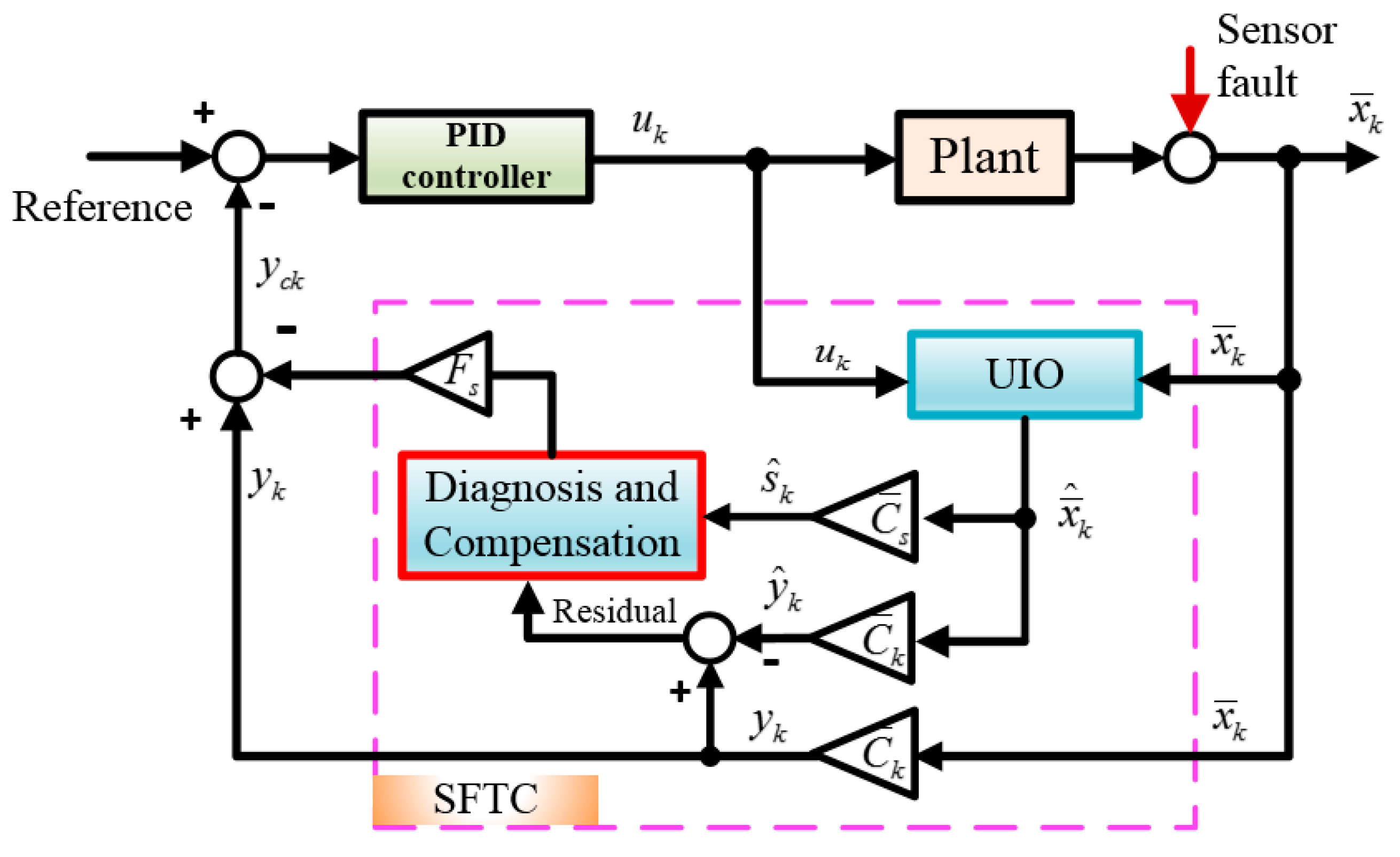
4. Sensor Fault-Tolerant Control in an MMP System

4.1. General Residual from the Sensor Fault Signal

Under the state estimation vector of the UIO, the residual vector is calculated as [12]:

$$r_k=y_k-{\widehat{y}}_k$$

(55)

This means that $r_k=0$ if $s_k=0$ and $r_k\ne 0$ if $s_k\ne 0$.

4.2. Sensor FTC Compensation

The sensor fault output from the measurements influences the closed-loop behavior and corrupts the state estimation.

The SFTC technique is designed based on the position SFs compensation to handle the sensor fault issues of the MMP system, as shown in Figure 2. The PID main controller will operate conventional close-loop trajectory control. The measurement is employed as [18]:

$$y_{ck}=y_k-F_s{\widehat{s}}_k$$

(56)

Fault compensation is operated by a logic process that is based on a residual via a threshold value k equal to 0 if $\left|r_k\right|\le k$, and equal to 1 if $\left|r_k\right|>k$ [12].

4.3. Simulation and Results

4.3.1. The parameters of the MMP system

The parameters of the MMP system were gathered from a KYB MMP4 by a cylinder of φ40 − φ20 − 250 and a motor of DC 24V. Some parameters were determined using the parameter estimation method in MATLAB version 2015a, 64 bits. The resulting parameters of the MMP system are shown in

Table 1. Basic parameters of the mini motion package (MMP) system.

Components	Values	Units
Ah	0.0013	m2
Ar	9.4e-4	m2
Vch	2.09e-4	m3
Vcr	4.0065e-05	m3
mp	10	kg
${\beta }_e$	2.9e+08	Pa
$K_{sp}$	2383	Nm
Dp	3.5e-6	m3

.

The basic parameters of the MMP system are listed in Table 1 as follows:

The matrices in (16) and (34) of the EHA system were obtained as:

$$B_k=\left[\begin{array}{ccc}0& 0& 0\end{array}\right]{\hspace{0.17em}}^T;C_k=\left[\begin{array}{ccc}1& 0& 0\end{array}\right];F_s=1;\hspace{0.17em}$$

$$A_k=\left[\begin{array}{ccc}1& 0.001& 0\\ 0& 0.9998& 0.0005\\ 0& -0.2911& 0.2311\end{array}\right]\hspace{0.17em}.$$

Based on [35], the sampling time $T_s$ can be selected by $T_s=1$ ms.

To investigate the MMP tracking control, without loss of generality, a reference trajectory for the positive position of the system cylinder was given as:

$$y_r=\sin (0.85t)+1.5$$

(57)

and a sensor fault $s(t)$ was simulated by the following function:

$$s(t)=\{\begin{array}{ll}0& \mathrm{if} t<2.945\\ 0.75\sin (8t)+1& \mathrm{if} 2.945\le t\le 3.9275\\ 0.75& \mathrm{if} 3.9275\le t\le 7\\ 2.55t-17.1& \mathrm{if} 7\le t\le 7.25\\ -2.55t+17.7& \mathrm{if} 7.25\le t\le 7.75\\ 0.8125t-6.034375& \mathrm{if} 8.75\le t\le 10\\ 0& \mathrm{if} t>10\end{array}$$

(58)

Based on the design experience, the positive scalars ζ, r, α, ε, and µ were selected as $\zeta =20$; $r=0.01$, $\alpha =0.1$, $\epsilon =0.1$, and $\mu =0.2$. The LMI defined by (45, 46) can be solved for $P_n$, $Q_n$, and $F_n$. If the solution is feasible, then the results can be obtained as:

$$\mathrm{\Sigma }=\left[\begin{array}{cccc}1& 0& 0& 0\\ 0& 1& 0& 0\\ 0& 0& 1& 0\\ -1& 0& 0& 0\end{array}\right];H=\left[\begin{array}{c}0\\ 0\\ 0\\ 1\end{array}\right];Q_n=\left[\begin{array}{l}-2.3626\mathrm{e}+0\\ \hspace{0.17em}0.1264\mathrm{e}-08\\ -3.1485\mathrm{e}-09\\ -2.3626\mathrm{e}+0\end{array}\right]\hspace{0.17em};$$

$$P_n=\left[\begin{array}{cccc}2.321\mathrm{e}+1 & -1.001\mathrm{e}-7& 2.965\mathrm{e}-8& 2.321\mathrm{e}+1\\ -1.001\mathrm{e}-7& 1.914\mathrm{e}-9 & 4.062\mathrm{e}-10& -1.001\mathrm{e}-7\\ 2.965\mathrm{e}-8& 4.062\mathrm{e}-10& 3.097\mathrm{e}-9 & 2.965\mathrm{e}-8\\ 2.321\mathrm{e}+1& -1.001\mathrm{e}-7& 2.965\mathrm{e}-8& 2.321\mathrm{e}+1\end{array}\right]\hspace{0.17em};$$

$$L_1=\left[\begin{array}{l}-6.2519\mathrm{e}+02\\ -9.3052\mathrm{e}-02\\ 9.2219\mathrm{e}-02\\ 6.2509\mathrm{e}+02\end{array}\right]\hspace{0.17em};L=\left[\begin{array}{l}-2.2737\mathrm{e}-13\\ -2.7756\mathrm{e}-17\\ 2.7756\mathrm{e}-17\\ 2.2737\mathrm{e}-13\hspace{0.17em}\end{array}\right];$$

$$F_n=\left[\begin{array}{cccc}6.262\mathrm{e}+2& 9.999\mathrm{e}-4& 3.244\mathrm{e}-7& 6.252\mathrm{e}+2\\ 9.305\mathrm{e}-2& 9.998\mathrm{e}-1& 5.250\mathrm{e}-4& 9.305\mathrm{e}-2\\ -9.222\mathrm{e}-2& -2.911\mathrm{e}-1& 2.311\mathrm{e}-1& -9.222\mathrm{e}-2\\ -6.261\mathrm{e}+2 & -9.999\mathrm{e}-4& -3.244\mathrm{e}-7& -6.251\mathrm{e}+2\end{array}\right]\hspace{0.17em}.$$

4.3.2. The Evaluated Equations of the PID Controller for the MMP System

To evaluate the PID controller’s efficiency, the control error is normally one of the most important factors to evaluate the PID controller.

Considering that a position control error estimation is calculated as:

$$e_{ck}=y_r-y_{ck}$$

(59)

a maximum error result $e_{ck\max }$ of the position control error $e_{ck}$ is computed as:

$$e_{ck\max }=y_{r\max }-y_{ck\max }$$

(60)

where $y_{r\max }$ and $y_{ck\max }$ are the maximum reference signal and the maximum response signal, respectively.

The error performance ${}^p{e}_{ck\max }$ of the PID controller of the position control error $e_{ck\max }$ is defined as:

$${}^p{e}_{ck\max }=\left(1-\frac{e_{ck\max }}{e_{s\max }}\right)100\%$$

(61)

where

$$e_{s\max }=s_{\max }-s_{\min }$$

with $s_{\max }$ and $s_{\min }$ being the maximum and minimum sensor fault s(t), respectively.

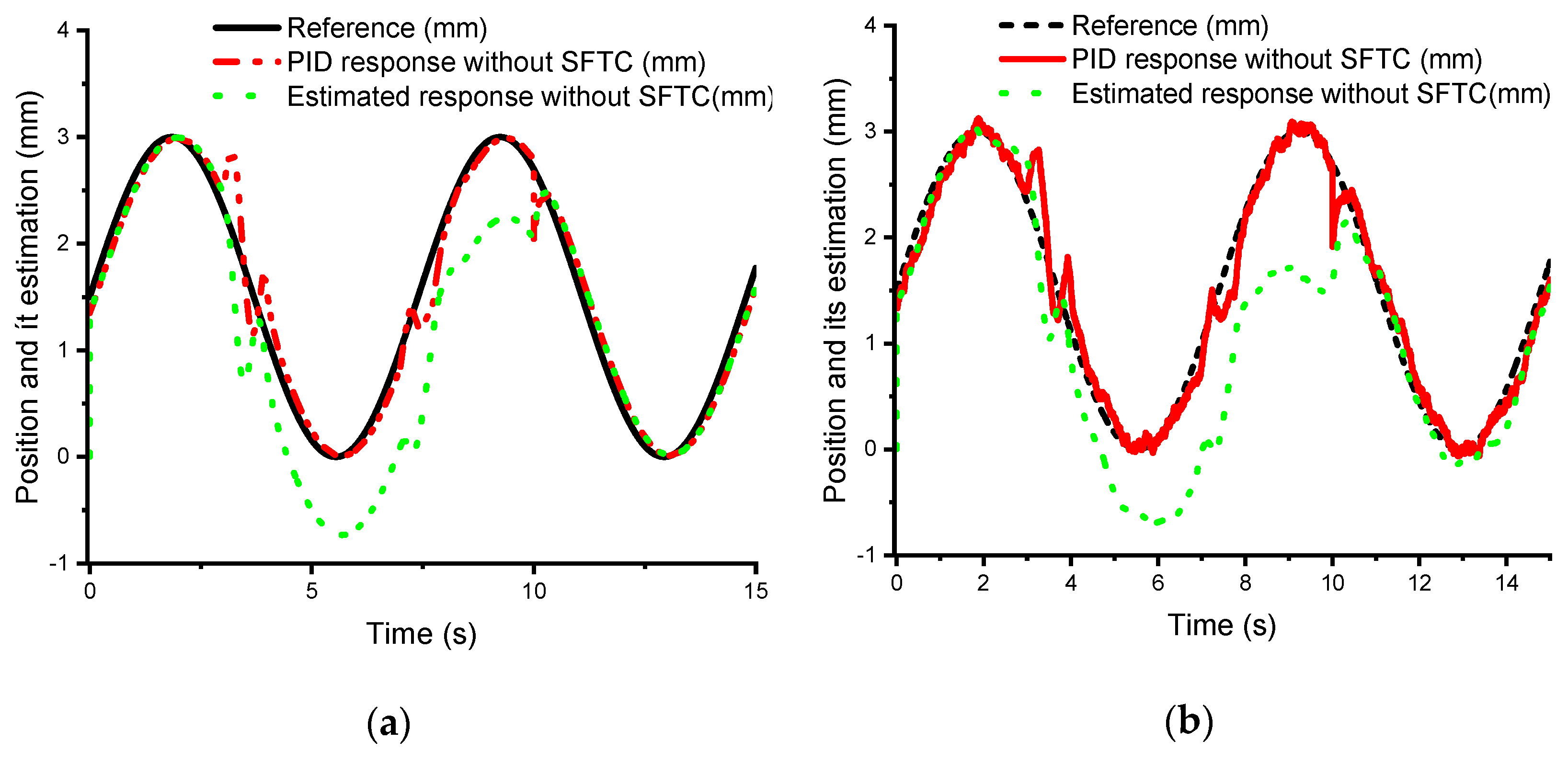
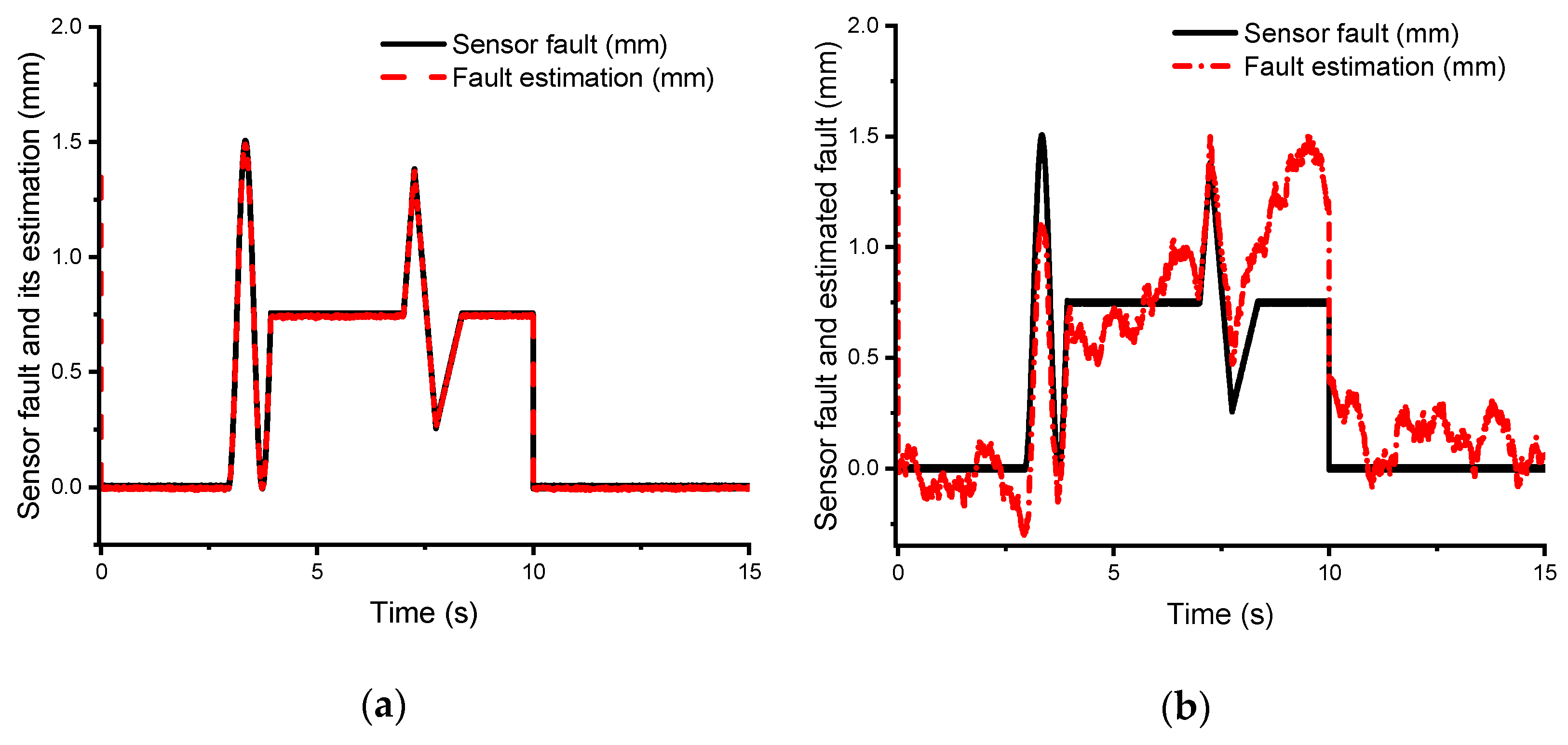
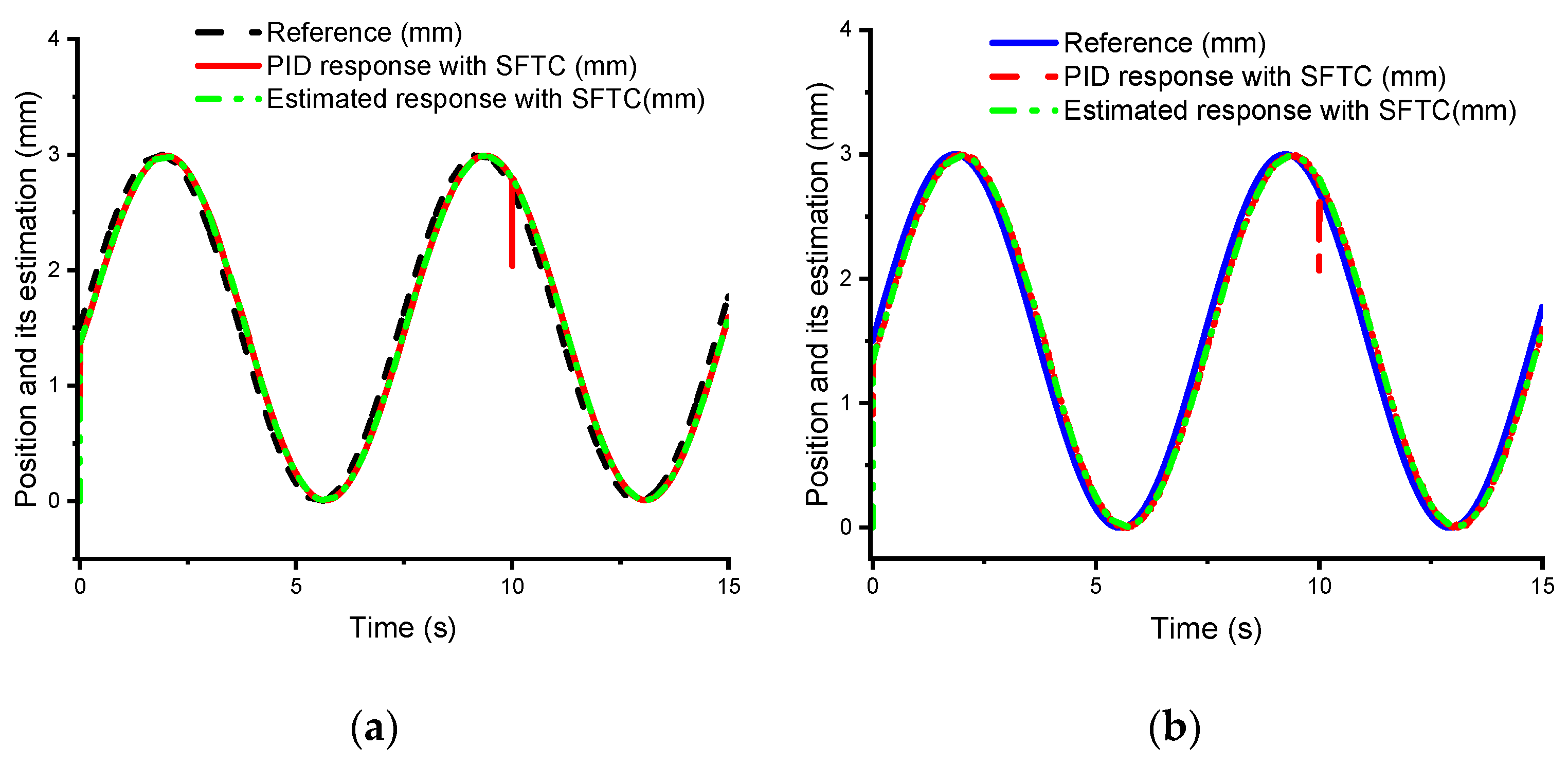
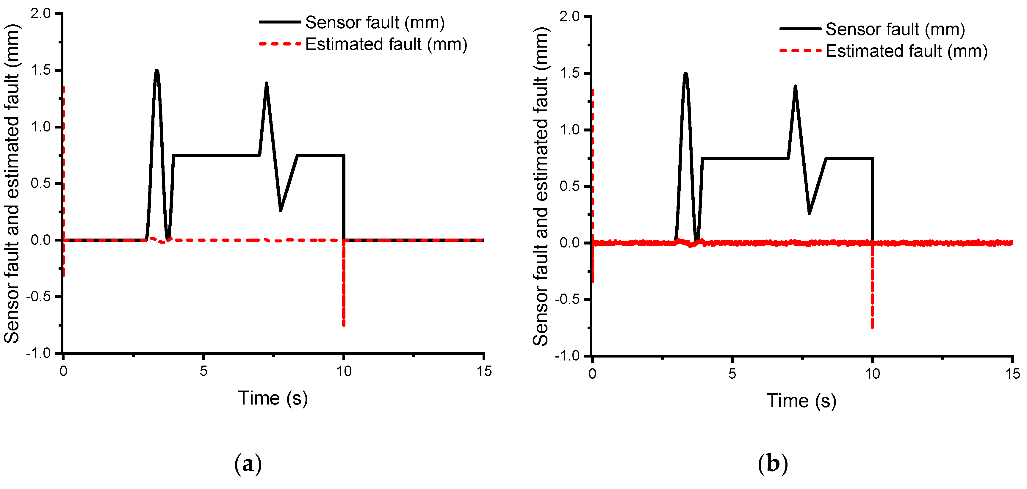
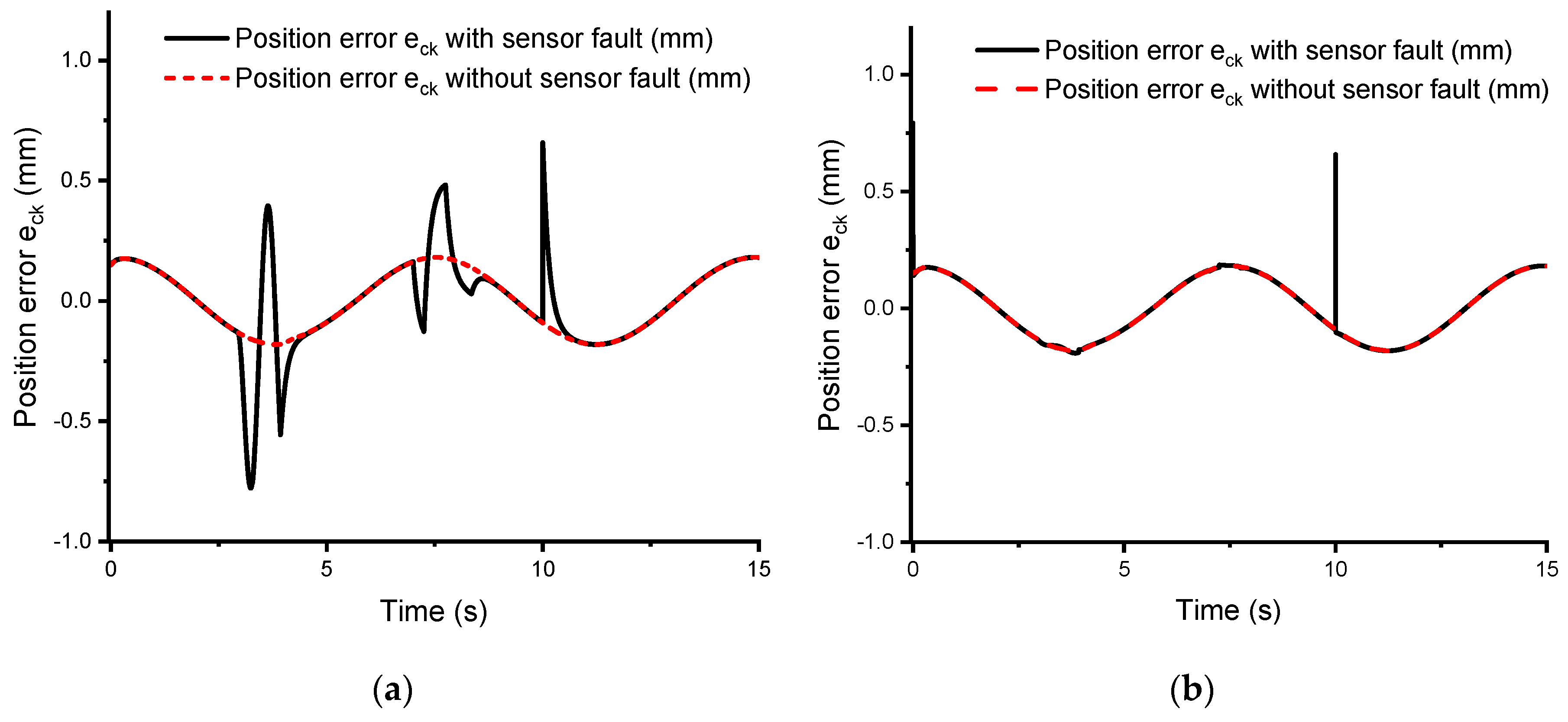
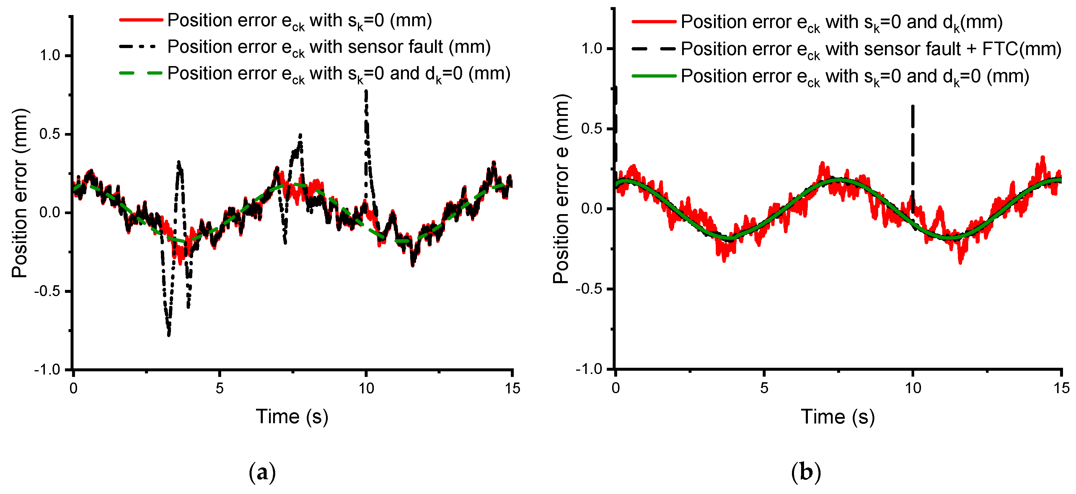
4.3.3. Simulation Results and Discussion

To assess the effectiveness of the developed control approach, we conducted a comparative simulation study on the system tracking performance, between the proposed SFTC and the traditional PID control without an FTC module. This control had been built in a MATLAB/Simulink environment, and a sampling time of T_s = 1ms was selected for all the simulations.

Numerical simulations were then carried out with the developed MMP model to follow the given trajectory (57) under the disturbed environment, including the faulty sensor condition (58) without disturbance ($d_k=0$), or with disturbance [$d_k=0.0045random(2,t)$]. By using the PID tuning tool of the Matlab Simulink toolbox, the parameters of the PID controller are obtained (K_P = 1.536, K_I = 1.32 and K_D = 0.0015) and applied to all the simulations.

The simulation results from Figure 3, Figure 4, Figure 5 and Figure 6 show that the PID response signal and its estimation signal followed the reference signal at locations without fault impacts, whereas when the SFTC was not applied for the system, these signals were affected by the fault at locations where the fault occurred (Figure 3a). In Figure 3a,b, the PID response signal without the SFTC clearly shows the effect of the unknown input disturbance. This influence of the fault estimation signal is similar to the sensor fault signal in Figure 3a, which demonstrates that the fault estimator of the system worked well. Nevertheless, there is the big difference between the fault estimation of Figure 3b compared with Figure 3a due to influences of the unknown input disturbance.

Figure 4a shows that the fault estimation signal reaches the sensor fault. This means that the fault estimator is performed well. Figure 4b shows the influences of disturbance to the fault estimation signal. The PID response signal and its estimation signal followed the reference signal when we applied the SFTC technology to our system even though the system is affected by the SFs in Figure 5a and unknown input disturbances in Figure 5b. Furthermore, the estimated fault can be reduced to zero when the SFTC technique is implemented by the compensation process, in cases with and without unknown inputs disturbance. Previous issues, to demonstrate that the MMP system works well when the proposed SFTC technology is utilized by the fault compensation process. Disturbances coming from an actuator are canceled after fault compensation; hence, we can use only the SFTC for fault compensation, which does not need an added actuator FTC for fault compensation.

In Figure 6a,b, the estimated error signal reaches zero value when the SFTC technology is used to perform error compensation.

To evaluate the PID controller performance, some data are listed in

Table 2. The error assessment $e_{ck\max }$ with disturbance $d_k=0$.

The Requirement Content	Without SFTC		With SFTC
	${\mathit{e}}_{\mathit{c}\mathit{k}\mathbf{max}}$ (mm)	${}^{\mathit{p}}{\mathit{e}}_{\mathit{c}\mathit{k}\mathbf{max}}$ (%)	${}^{\mathit{f}\mathit{t}\mathit{c}}{\mathit{e}}_{\mathit{c}\mathit{k}\mathbf{max}}$ (mm)	${}^{\mathit{p}}{\mathit{e}}_{\mathit{c}\mathit{k}\mathbf{max}}$ (%)
From 0.2 s to 5 s	1.194	20.67	0.0194	98.06
From 5 s to 9 s	0.6074	34.9	0.0149	98.51
From 0.2 s to 9 s	1.194	27.79	0.0194	98.26
From 9 s to 15 s	0.7511	24.89	0.7515	24.50

. Here, the control error result $e_{ck}$ is compared between cases with and without sensor faults in Figure 7a. Moreover, the superior performance of the proposed SFTC compared with the traditional tracking controller PID is evidenced by the difference between the control error $e_{ck}$ without SFTC and the control error $e_{ck}$ with SFTC, which is described in Table 2 and displayed in Figure 7a,b. The error performance ${}^p{e}_{ck\max }$ of the PID controller with the SFTC averaged about 98.258% from 0.2 s to 9 s, whereas it averaged about 27.785% without the SFTC (Table 2). In contrast, the control error barely changed from 9 s to 15 s, even though there were fewer errors with the SFTC. This can be explained by the fact that the compensation process is executed in the second step of two adjacent steps. Therefore, signals with a vertical direction change will not be performed for compensation, as can be seen in Figure 5a,b at time 10 s.

Table 3. The error assessment $e_{ck\max }$ using a PID controller with disturbance $d_k$.

Content	Without SFTC				With SFTC
	${\mathit{d}}_{\mathit{k}}=0$		With ${\mathit{d}}_{\mathit{k}}$		${\mathit{d}}_{\mathit{k}}=0$		With ${\mathit{d}}_{\mathit{k}}$
	${\mathit{e}}_{\mathit{c}\mathit{k}\mathbf{max}}$ (mm)	${}^{\mathit{p}}{\mathit{e}}_{\mathit{c}\mathit{k}\mathbf{max}}$ (%)	${\mathit{e}}_{\mathit{c}\mathit{k}\mathbf{max}}$ (mm)	${}^{\mathit{p}}{\mathit{e}}_{\mathit{c}\mathit{k}\mathbf{max}}$ (%)	${}^{\mathit{f}\mathit{t}\mathit{c}}{\mathit{e}}_{\mathit{c}\mathit{k}\mathbf{max}}$ (mm)	${}^{\mathit{p}}{\mathit{e}}_{\mathit{c}\mathit{k}\mathbf{max}}$ (%)	${}^{\mathit{f}\mathit{t}\mathit{c}}{\mathit{e}}_{\mathit{c}\mathit{k}\mathbf{max}}$ (mm)	${}^{\mathit{p}}{\mathit{e}}_{\mathit{c}\mathit{k}\mathbf{max}}$ (%)
From 0.2 s to 5 s	1.1940	20.67	1.1181	25.46	0.0194	98.06	0.3961	73.60
From 5 s to 9 s	0.6074	34.9	0.7154	28.46	0.0149	98.51	0.3003	69.97
From 0.2 s to 9 s	1.1940	27.79	1.1181	26.96	0.0194	98.26	0.3961	71.76
From 9 s to 15 s	0.7511	24.89	1.1188	-11.88	0.7515	24.50	0.8654	13.46

summarizes the position control error $e_{ck\max }$ of the PID controller under an unknown input disturbance $d_k$ condition, with and without SFTC. In the case with disturbance $d_k$, from 0.2 s to 9 s, the average performance of the PID controller decreased by 0.83% (from 27.79% to 26.96%) without an SFTC and by 26.5% (from 98.26% to 71.76%) with an SFTC due to the effect of the disturbance. The PID controller performance was strongly decreased, from 24.89% to -11.88%, from 9 s to 15 s without an SFTC and from 24.50% to 13.46% with an SFTC (Figure 8a,b).

5. Conclusions

In this paper, an advanced SFTC technique is developed for a class of nonlinear discrete-time systems. This technique is successfully applied to control the position of an MMP system with sensor faults and an unknown input disturbance. The developed control technique, including SFs and system disturbances, is first estimated using the UIO and an LMI optimization algorithm. The estimated signals are utilized to generate compensation control to overcome the control challenges. By using the proposed SFTC, the system output follows the desired trajectory very well, even under the disturbed environment and concurrent sensor faults. Simulations are carried out to demonstrate the superior performance of the proposed SFTC technique over the traditional control method without fault-tolerant control features, as summarized in Table 2. With the SFTC technique, the control performance is determined to be 98.26% for the case without disturbance $d_k$ and 71.76% for the case of disturbance $d_k$, as shown in Table 3. In future work, practical experiments with the developed rig will be carried out to confirm the applicability of the developed SFTC approach in real-time.

References and Notes

1. Nam, K.; Cho, K.; Park, S.S. Design and Performance Evaluation of an Electro-Hydraulic Camless Engine Valve Actuator for Future Vehicle Applications. Sensors 2017, 17, 2940. [Google Scholar] [CrossRef] [PubMed]
2. Liu, C.; Jiang, H. A seventh-order model for dynamics response of an electro-hydraulic servo valve. Chin. J. Aeronaut. 2014, 27, 1605–1611. [Google Scholar] [CrossRef]
3. Truong, Q.D.; Ahn, K.K. Force control for press machines using an online smart tuning fuzzy PID based on a robust extended Kalman filter. Expert Syst. Appl. 2011, 38, 5879–5894. [Google Scholar] [CrossRef]
4. Rahmat, F.M.; Husain, A.R.; Ishaque, K.; Sam, Y.M.; Ghazali, R.; Rozali, S.M. Modeling and controller design of an industrial hydraulic actuator system in the presence of friction and internal leakage. Int. J Phys. Sci. 2011, 6, 3502–3517. [Google Scholar] [CrossRef]
5. Ahn, K.K.; Nam, D.N.C.; Jin, M. Adaptive Back-stepping Control of an Electrohydraulic Actuator. IEEE/ASME Trans. Mechatron. 2014, 19, 987–995. [Google Scholar] [CrossRef]
6. Tri, M.N.; Nam, C.N.D.; Park, G.H.; Ahn, K.K. Trajectory control of an electro-hydraulic actuator using an iterative backstepping control scheme. Mechatronics 2014, 29, 96–102. [Google Scholar] [CrossRef]
7. Law, M.; Wabner, M.; Colditz, A.; Kolouch, M.; Noack, S.; Ihlenfeldt, S. Active vibration isolation of machine tools using an electro-hydraulic actuator. CIRP J. Manuf. Sci. Technol. 2015, 10, 36–48. [Google Scholar] [CrossRef]
8. Ijaz, S.L.; Ashraf, M.A.; Mumtaz, M.F.; Ali, Y.; Baig, W.M. Fixed structured H∞controller design for aircraft control surface driven by power by wire hydraulic actuator. In Proceedings of the 2017 14th International Bhurban Conference on Applied Sciences and Technology (IBCAST), Islamabad, Pakistan, 10–14 January 2017; pp. 259–264. [Google Scholar] [CrossRef]
9. Di Rito, G.; Denti, E.; Galatolo, R. Robust force control in a hydraulic workbench for flight actuators. In Proceedings of the 2006 IEEE Conference on Computer Aided Control System Design, 2006 IEEE International Conference on Control Applications, 2006 IEEE International Symposium on Intelligent Control, Munich, Germany, 4–6 October 2006; pp. 807–813. [Google Scholar] [CrossRef]
10. Mohammad, A.; Danish, M.S.; Yuvraj, G.P.; Shubham, P.K. A Study on Landing Gear Arrangement of an Aircraft. Int. J. Innov. Res. Sci. Eng. Technol. 2017, 6, 2347–6710. [Google Scholar] [CrossRef]
11. Ayman, A.A. Model Reference PID Control of an Electrohydraulic Drive. Int. J. Intell. Syst. Appl. 2012, 11, 24–32. [Google Scholar] [CrossRef]
12. Noura, H.; Theilliol, D.; Ponsart, J.C.; Chamseddine, A. Fault-Tolerant Control Systems Design and Practical Applications; Michael, J.G., Michael, A.J., Eds.; Springer: Dordrecht, The Netherlands; Heidelberg, Germany; London, UK; New York, NY, USA, 2009; ISBN 978-1-84882-652-6. [Google Scholar] [CrossRef]
13. Navid, N.; Nariman, S. A QFT Fault-Tolerant Control for Electrohydraulic Positioning Systems. IEEE Trans. Mechatron. 2002, 10, 626–632. [Google Scholar] [CrossRef]
14. Fikret, C.; Chingiz, H. Active Fault-Tolerant Control of UAV Dynamics against Sensor-Actuator Failures. J. Aerosp. Eng. 2016, 29, 04016012. [Google Scholar] [CrossRef]
15. Jing, H.; Lin, M.; Songan, M.; Changfan, Z.; Houguang, C. Fault-Tolerant Control of a Nonlinear System Actuator Fault Based on Sliding Mode Control. J. Control Sci. Eng. 2017. [Google Scholar] [CrossRef]
16. Sami, M.; Patton, R.J. Active fault tolerant control for nonlinear systems with simultaneous actuator and sensor faults. Int. J. Control Autom. Syst. 2013, 11, 1149. [Google Scholar] [CrossRef]
17. Noura, H.; Sauter, D.; Hamelin, F.; Theilliol, D. Fault-tolerant control in dynamic systems: Application to a winding machine. IEEE Control Syst. Mag. 2000, 20, 33–49. [Google Scholar] [CrossRef]
18. Liu, X.; Gao, Z.; Zhang, A. Robust Fault Tolerant Control for Discrete-Time Dynamic Systems with Applications to Aero Engineering Systems. IEEE Access 2018, 6, 18832–18847. [Google Scholar] [CrossRef]
19. Dongsheng, D.; Vincent, C. Fault diagnosis and fault tolerant control for discrete-time linear systems with sensor fault. IFAC-PapersOnLine 2017, 50, 15754–15759. [Google Scholar] [CrossRef]
20. Nahian, A.S.; Truong, D.Q.; Chowdhury, P.; Das, D.; Ahn, K.K. Modeling and Fault Tolerant Control of an ElectroHydraulic Actuator. Int. J. Precis. Eng. Manuf. 2016, 17, 1285–1297. [Google Scholar] [CrossRef]
21. Halim, A.; Christopher, E.; Chee, P.T. Fault Detection and Fault-Tolerant Control Using Sliding Modes; Springer: London, UK, 2011; ISBN 978-0-85729-649-8. [Google Scholar]
22. Hamed, H.; Ian, H.; Silvio, S. Reliability improvement of wind turbine power generation using model-based fault detection and fault tolerant control: A. review. Renew. Energy 2019, 135, 877–896. [Google Scholar] [CrossRef]
23. Bahareh, P.; Nader, M.; Khashayar, K. Sensor Fault Detection, Isolation and Identification Using Multiple Model-based Hybrid Kalman Filter for Gas Turbine Engines. IEEE Trans. Control Syst. Technol. 2016, 24, 1184–1200. [Google Scholar] [CrossRef]
24. Jian, Z.; Akshya, K.S.; Sing, K.N. Robust Observer-Based Fault Diagnosis for Nonlinear Systems Using MATLAB. In Advances in Industrial Control; Michael, J.G., Michael, A.J., Eds.; Springer International Publishing: Basel, Switzerland, 2016; ISBN 978-3-319-32323-7. [Google Scholar] [CrossRef]
25. Zhang, K.; Jiang, B.; Shi, P. Adjustable Parameter-Based Distributed Fault Estimation Observer Design for Multiagent Systems with Directed Graphs. IEEE Trans. Cybern. 2017, 47, 306–314. [Google Scholar] [CrossRef]
26. Gao, Z.; Breikin, T.; Wang, H. High-Gain Estimator and Fault-Tolerant Design with Application to a Gas Turbine Dynamic System. IEEE Trans. Control Syst. Technol. 2007, 15, 740–753. [Google Scholar] [CrossRef]
27. Liu, X.; Gao, Z. Novel unknown input observer for fault estimation of gas turbine dynamic systems. In Proceedings of the 2015 IEEE 13th International Conference on Industrial Informatics (INDIN), Cambridge, UK, 22–24 July 2015; pp. 562–567. [Google Scholar] [CrossRef]
28. Gao, Z.; Ding, X.S. Sensor fault reconstruction and sensor compensation for a class of nonlinear state-space systems via a descriptor system approach. IET Control Theory Appl. 2007, 1, 578–585. [Google Scholar] [CrossRef]
29. Jia, Q.; Li, H.; Zhang, Y.; Chen, X. Robust observer-based sensor fault reconstruction for discrete-time systems via a descriptor system approach. Int. J. Control Autom. Syst. 2015, 13, 274. [Google Scholar] [CrossRef]
30. Khosrowjerdi, M.J. Robust Sensor Fault Reconstruction for Lipschitz Nonlinear Systems. Math. Prob. Eng. 2011. [Google Scholar] [CrossRef]
31. Damianno, R.; Fatiha, N.; Vicenc, P. Robust QUASI–LPV Mode Reference FTC of a Quadrotor UAV Subject to Actuator Fauts. Int. J. Appl. Math. Comput. Sci. 2015, 25, 7–22. [Google Scholar] [CrossRef]
32. Abderrahmen, B.; Djamel, S.; Kamel, K.; Samir, Z. Fault-Tolerant Lyapunov-Gain-Scheduled PID Control of a Quadrotor UAV. Int. J. Intell. Eng. Syst. 2015, 8. [Google Scholar] [CrossRef]
33. Equations are used from the help tool Matlab 2017b version.
34. Boyd, S.; Ghaoui, L.E.; Feron, E.; Balakrishnan, V. Linear Matrix Inequalities in Systems and Control Theory; SIAM: Philadelphia, PA, USA, 1994; ISBN 0-89871-334-X. [Google Scholar]
35. Sofiane, A.A.; Arnaud, C.; Steven, B.; Nicolag, L. Continuous-Discrete Time-Observer Design for State and Disturbance Estimation of Electro-Hydraulic Actuator Systems. IEEE Trans. Ind. Electron. 2016. [Google Scholar] [CrossRef]
Figure 1. Schematic of an electro-hydraulic actuator (EHA) system.
Processes 07 00089 g001
Figure 2. The structure of observer-based fault-tolerant control.
Processes 07 00089 g002
Figure 3. Position response and its estimation without SFTC of (a) disturbance d k = 0 , and (b) disturbance d k = 0.0045random(2,t).
Processes 07 00089 g003
Figure 4. Sensor fault and its estimation without SFTC (a) disturbance d k = 0 , and (b) disturbance d k = 0.0045random(2,t).
Processes 07 00089 g004
Figure 5. Position response and its estimation with SFTC (a) disturbance d k = 0 , and (b) disturbance d k = 0.0045random(2,t).
Processes 07 00089 g005
Figure 6. Sensor fault and its estimation with SFTC (a) disturbance d k = 0 , and (b) disturbance d k = 0.0045random(2,t).
Processes 07 00089 g006
Figure 7. The position control error e c k for the case without disturbance d k of (a) without SFTC, and (b) with SFTC.
Processes 07 00089 g007
Figure 8. The position control error e c k with disturbance d k of (a) without SFTC, and (b) with SFTC.
Processes 07 00089 g008