Titanium Distribution Ratio Model of Ladle Furnace Slags for Tire Cord Steel Production Based on the Ion–Molecule Coexistence Theory at 1853 K

Abstract

High-strength tire cord steel is mainly used in radial ply tires, but the presence of brittle Ti inclusions can cause failure of the wires and jeopardize their performance in production. In order to control the titanium content during steel production, a thermodynamic model for predicting the titanium distribution ratio between CaO–SiO₂–Al₂O₃–MgO–FeO–MnO–TiO₂ slags during the ladle furnace (LF) refining process at 1853 K has been established based on the ion–molecule coexistence theory (IMCT), combined with industrial measurements, and the effect of basicity on the titanium distribution ratio was discussed. The results showed that the titanium distribution ratio predicted by the developed IMCT exhibited a dependable agreement with the measurements, and the optical basicity is suggested to reflect the correlation between basicity and the titanium distribution ratio. Furthermore, quantitative titanium distribution ratios of TiO₂, CaO·TiO₂, MgO·TiO₂, FeO·TiO₂, and MnO·TiO₂ were acquired by the IMCT model, respectively. Calculation results revealed that the structural unit CaO plays a pivotal role in the slags in the de-titanium process.

1. Introduction

Titanium is a common microalloy addition to steels. It can be used to inhibit grain growth, reduce the incidence of transverse cracking in niobium-containing steels production, stabilize the alloy against sensitization to intergranular corrosion, and improve the service performance [1,2,3,4]. However, a low titanium content is demanded for special kinds of steel production, such as in high-strength tire cord steel, to enhance drawing and twisting performances.

As a product with superior quality to wire rods, tire cord steel is mainly used in radial ply tires. Before it is made, the steel wire is drawn from 5.5 mm to 0.15 mm in diameter and subjected to cyclic stress in the drawing and twisting process. Therefore, breakage of steel wire during fabrication is a crucial issue. This filament break is especially sensitive with the existence of angular and non-deformable Ti inclusions, such as titanium nitride (TiN) or titanium carbonitride (Ti(CN)) [5,6,7,8,9]. This causes a decrease in fatigue performance and can seriously affect traffic safety.

Therefore, the issue of the control of titanium content has received considerable critical attention. To control the titanium content during steel production, it is essential to study the titanium distribution ratio between steel and slag. To date, there has been limited theoretical and experimental studies implemented on the titanium distribution behavior in slags; acquiring relevant parameters at elevated temperatures between steel and slag is arduous and costly. It is quite essential to establish a thermodynamic model for calculating the titanium distribution ratio between steel and slag. The ion–molecule coexistence theory (IMCT) has been efficaciously applied to describe phosphate capacity, manganese distribution, sulfide capacity, and so on, as shown in

Table 1. Applications of the ion–molecule coexistence theory (IMCT) model during ironmaking and steelmaking processes.

Slag Systems	Applications	Ref.
CaO–SiO2–FeO–MgO–MnO–Al2O3	A thermodynamic model for predicting the manganese distribution ratio and manganese capacity of the slags was developed based on the IMCT. The established model was successfully applied to not only manganese equilibrium experiments but also industrial production.	[10]
CaO–SiO2–MgO–FeO–MnO–Al2O3–TiO2–CaF2	A thermodynamic model for calculating the manganese distribution ratio between the slags and carbon saturated liquid iron was built based on the IMCT. The predicted manganese distribution ratio by IMCT had a good linear relationship with measurements expect individual points.	[11]
CaO–SiO2–MgO–FeO–Fe2O3–Al2O3–P2O5	A thermodynamic model for predicting the phosphorus distribution ratio of the slags was developed based on the IMCT. The developed model was successfully applied to not only phosphorus equilibrium experiments, but also industrial production in Hismelt smelting reduction vessels.	[12]
CaO-based Slags	A thermodynamic model for predicting phosphorus partition between CaO-based slags during hot metal dephosphorization pretreatment was established based on the IMCT. The established model was verified as effective through comparing with measured results and predicted ones by other models.	[13]
CaO–SiO2–MgO–FeO–Fe2O3–MnO–Al2O3–P2O5	A thermodynamic model for calculating the phosphorus distribution ratio between steelmaking slags and molten steel was built based on the IMCT. The built IMCT prediction model was verified with measured and some other reported models.	[14]
CaO–FeO–Fe2O3–Al2O3–P2O5	Thermodynamic models for predicting the phosphorus distribution ratio and phosphorus capacity of the slags during refining were developed based on the IMCT. The developed models were verified with experimental results and reported models.	[15]
CaO–SiO2–FeO–Fe2O3–P2O5	Defined enrichment possibility and enrichment degree of solid solutions containing P2O5 from the developed IMCT model were verified from experimental results.	[16]
CaO-based Slags	Coupling relationships between dephosphorization and desulfurization abilities or potentials for CaO-based slags during the refining process of molten steel were proposed based on the IMCT. The proposed model was verified as effective and feasible through investigating the effect of slag composition.	[17]
CaO–SiO2–MgO–Al2O3	A sulfide capacity prediction model of the slags was developed based on the IMCT. The developed model had a higher accuracy than other reported sulfide capacity prediction models.	[18]
CaO–SiO2–MgO–FeO–MnO–Al2O3	A thermodynamic model for calculating the sulfur distribution ratio between ladle furnace (LF) refining slags and molten steel was established based on the IMCT. The model was verified with the measured and the calculated sulfur distribution ratio by Young’s model and the KTH model in LF refining.	[19]
CaO–SiO2–MgO–FeO–MnO–Al2O3	A sulfide capacity prediction model of the LF refining slags was built based on the IMCT. The built sulfide capacity prediction model was verified with the measured and calculated by Young’s model and the KTH model in LF refining.	[20]
CaO–FeO–Fe2O3–Al2O3–P2O5	A thermodynamic model for predicting the sulfide capacity of the slags at various oxygen potentials was developed based on the IMCT. The built model was verified through comparing the determined sulfide capacity, and could be applied to precisely predict sulfide capacity.	[21]
CaO–FeO–Fe2O3–Al2O3–P2O5	A thermodynamic model for predicting the sulfur distribution ratio between the slags and liquid iron was built based on the IMCT. The developed model was verified with measured data of sulfur distribution equilibrium from the literatures.	[22]
CaO–SiO2–MgO–FeO–Fe2O3–MnO–Al2O3–P2O5	The defined oxidation ability of metallurgical slags based on the IMCT was verified by comparisons with the reported activity in the selected FetO-containing slag systems.	[23]

[10,11,12,13,14,15,16,17,18,19,20,21,22,23]. In the IMCT, the defined mass action–concentration (MAC) is consistent with the classical concept of activity in the slag.

To improve the application domain of IMCT, in this paper, a titanium distribution ratio model of CaO–SiO₂–Al₂O₃–MgO–FeO–MnO–TiO₂ slags was built based on the IMCT, combined with industrial measurements. From the results, the titanium distribution behavior during ladle furnace (LF) refining in high-strength tire cord steel production is further revealed.

2. Materials and Methods

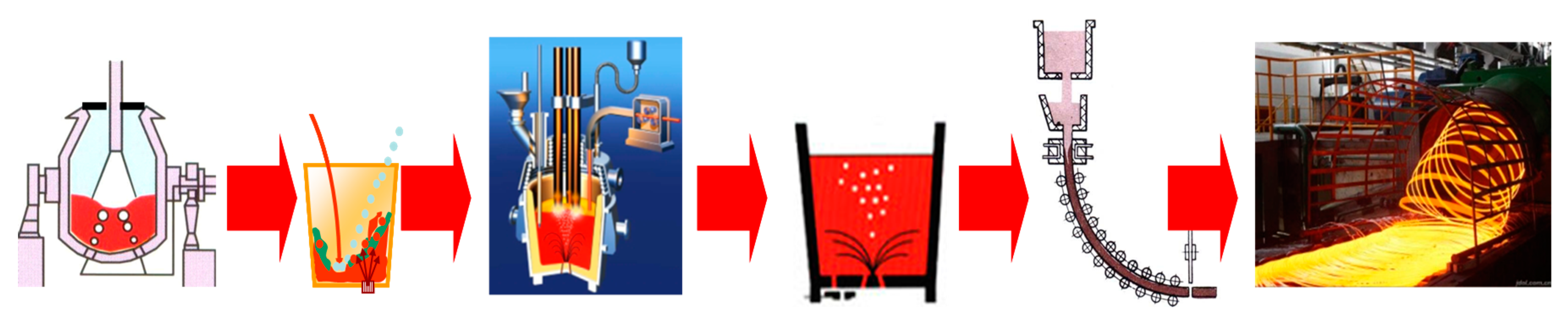
2.1. Production Procedure and Materials

The following process was adopted for the production of high-strength tire cord steel in Baosteel (Wuhan Branch): basic oxygen furnace (BOF) → tapping → ladle furnace (LF) → soft blowing → continuous casting (CC) → rolling. Figure 1 shows a schematic diagram of the production process.

Both the liquid steel and balanced slag were sampled at the end point of the LF refining process at about 1853 K. The orthonormal chemical components of molten steel and slags for 16 heats are given in

Table 2. Chemical components of liquid steel and slags at the end point of LF refining (wt %).

Slag Composition							Metal Composition
CaO	SiO2	Al2O3	MgO	FeO	MnO	TiO2	C	Si	Mn	Ti
39.19	40.50	7.97	8.47	1.36	2.17	0.34	0.81	0.20	0.47	0.0008
38.56	40.95	7.73	8.89	1.27	2.28	0.31	0.80	0.19	0.48	0.0008
35.19	43.10	6.82	10.79	1.41	2.52	0.18	0.83	0.18	0.46	0.0006
34.70	42.92	6.46	10.97	1.81	2.95	0.19	0.80	0.20	0.46	0.0007
39.47	41.52	7.19	8.17	1.61	1.78	0.25	0.80	0.20	0.45	0.0006
37.08	45.82	3.78	8.10	1.61	3.40	0.20	0.82	0.20	0.46	0.0007
34.28	45.19	6.07	11.09	1.36	1.69	0.33	0.82	0.19	0.47	0.0012
36.11	44.54	4.79	9.12	1.73	3.49	0.22	0.81	0.18	0.46	0.0008
40.04	39.73	8.87	8.38	1.28	1.38	0.32	0.82	0.18	0.48	0.0007
33.25	45.28	7.74	10.12	1.62	1.71	0.27	0.80	0.19	0.47	0.0012
34.52	47.74	3.52	10.72	1.11	2.14	0.25	0.81	0.19	0.46	0.0010
37.23	43.69	6.48	9.12	1.34	1.86	0.28	0.82	0.20	0.47	0.0008
42.90	43.04	5.46	5.98	1.00	1.29	0.33	0.80	0.18	0.45	0.0007
36.52	46.23	4.75	8.65	1.14	2.44	0.26	0.83	0.20	0.46	0.0009
34.51	46.01	5.54	10.61	0.94	2.14	0.24	0.80	0.19	0.46	0.0009
31.73	45.69	6.82	9.78	1.08	4.70	0.21	0.81	0.20	0.48	0.0010

.

2.2. Establishment of the IMCT Model

Based on the assumptions inherent in the IMCT, the dominant features of the IMCT model for the activities of the structural units in the slag can be summarized briefly as follows:

(1)

The constitutional units in the slag consist of simple ions, ordinary molecules, and complicated molecules;

(2)

Complex molecules are generated by the reactions of bonded ion couples and simple molecules under kinetic equilibrium;

(3)

The activity of each constituent in the slag equals the MAC of the structural unit at the steelmaking temperature;

(4)

The chemical reactions comply with the law of mass conservation.

The calculations were based on actual production involving CaO–SiO₂–Al₂O₃–MgO–FeO– MnO–TiO₂ slag systems. The initial numbers of moles for each composition in 100 g of CaO–SiO₂–Al₂O₃–MgO–FeO–MnO–TiO₂ slag were $a=n_{\mathrm{CaO}}^0$, $b=n_{{\mathrm{SiO}}_2}^0$, $c=n_{{\mathrm{Al}}_2{\mathrm{O}}_3}^0$, $d=n_{\mathrm{MgO}}^0$, $e=n_{\mathrm{FeO}}^0$, $f=n_{\mathrm{MnO}}^0$, and $g=n_{{\mathrm{TiO}}_2}^0$, respectively. The balanced mole number of each constituent unit in the slag was defined as $n_i$, and N_i denotes the MAC of each constitutional unit. The MAC is equivalent to the classical definition of activity based on the IMCT and can be acquired as

$$N_i=\frac{n_i}{{\displaystyle \sum }{n}_i}$$

(1)

where ${\displaystyle \sum }{n}_i$ is the total mole number of each constitutional unit in equilibrium.

According to the IMCT, at 1853 K, the slag system contains five simple ions (Ca²⁺, Fe²⁺, Mg²⁺, Mn²⁺, and O²⁻) and three ordinary molecules (${\mathrm{Al}}_2{\mathrm{O}}_3$, ${\mathrm{SiO}}_2$, and ${\mathrm{TiO}}_2$). Based on the reported phase diagrams, 44 types of complex molecules can be generated at the steelmaking temperature [24,25]. The abovementioned structural units and their parameters are listed in

Table 3. Parameters of structural units in the slag system at 1853 K.

Items	Constitutional Units	Balanced Mole Number	MACs
Simple cations and anions	${\mathrm{Ca}}^{2+}+{\mathrm{O}}^{2-}$	$n_1=n_{{\mathrm{Ca}}^{2+}}=n_{{\mathrm{O}}^{2-}}=n_{\mathrm{CaO}}$	$N_1=\frac{2n_1}{{\displaystyle \sum }{n}_i}=N_{\mathrm{CaO}}$
	${\mathrm{Mg}}^{2+}+{\mathrm{O}}^{2-}$	$n_4=n_{{\mathrm{Mg}}^{2+}}=n_{{\mathrm{O}}^{2-}}=n_{\mathrm{MgO}}$	$N_4=\frac{2n_4}{{\displaystyle \sum }{n}_i}=N_{\mathrm{MgO}}$
	${\mathrm{Fe}}^{2+}+{\mathrm{O}}^{2-}$	$n_5=n_{{\mathrm{Fe}}^{2+}}=n_{{\mathrm{O}}^{2-}}=n_{\mathrm{FeO}}$	$N_5=\frac{2n_5}{{\displaystyle \sum }{n}_i}=N_{\mathrm{FeO}}$
	${\mathrm{Mn}}^{2+}+{\mathrm{O}}^{2-}$	$n_6=n_{{\mathrm{Mn}}^{2+}}=n_{{\mathrm{O}}^{2-}}=n_{\mathrm{MnO}}$	$N_6=\frac{2n_6}{{\displaystyle \sum }{n}_i}=N_{\mathrm{MnO}}$
Simple molecules	${\mathrm{SiO}}_2$	$n_2=n_{{\mathrm{SiO}}_2}$	$N_2=\frac{n_2}{{\displaystyle \sum }{n}_i}=N_{{\mathrm{SiO}}_2}$
	${\mathrm{Al}}_2{\mathrm{O}}_3$	$n_3=n_{{\mathrm{Al}}_2{\mathrm{O}}_3}$	$N_3=\frac{n_3}{{\displaystyle \sum }{n}_i}=N_{{\mathrm{Al}}_2{\mathrm{O}}_3}$
	${\mathrm{TiO}}_2$	$n_7=n_{{\mathrm{TiO}}_2}$	$N_7=\frac{n_7}{{\displaystyle \sum }{n}_i}=N_{{\mathrm{TiO}}_2}$
Complex molecules	$\mathrm{CaO}·{\mathrm{SiO}}_2$	$n_8=n_{\mathrm{CaO}·{\mathrm{SiO}}_2}$	$N_8=\frac{n_8}{{\displaystyle \sum }{n}_i}=N_{\mathrm{CaO}·{\mathrm{SiO}}_2}$
	$3\mathrm{CaO}·2{\mathrm{SiO}}_2$	$n_9=n_{3\mathrm{CaO}·2{\mathrm{SiO}}_2}$	$N_9=\frac{n_9}{{\displaystyle \sum }{n}_i}=N_{3\mathrm{CaO}·2{\mathrm{SiO}}_2}$
	$2\mathrm{CaO}·{\mathrm{SiO}}_2$	$n_{10}=n_{2\mathrm{CaO}·{\mathrm{SiO}}_2}$	$N_{10}=\frac{n_{10}}{{\displaystyle \sum }{n}_i}=N_{2\mathrm{CaO}·{\mathrm{SiO}}_2}$
	$3\mathrm{CaO}·{\mathrm{SiO}}_2$	$n_{11}=n_{3\mathrm{CaO}·{\mathrm{SiO}}_2}$	$N_{11}=\frac{n_{11}}{{\displaystyle \sum }{n}_i}=N_{3\mathrm{CaO}·{\mathrm{SiO}}_2}$
	$3\mathrm{CaO}·{\mathrm{Al}}_2{\mathrm{O}}_3$	$n_{12}=n_{3\mathrm{CaO}·{\mathrm{Al}}_2{\mathrm{O}}_3}$	$N_{12}=\frac{n_{12}}{{\displaystyle \sum }{n}_i}=N_{3\mathrm{CaO}·{\mathrm{Al}}_2{\mathrm{O}}_3}$
	$12\mathrm{CaO}·7{\mathrm{Al}}_2{\mathrm{O}}_3$	$n_{13}=n_{12\mathrm{CaO}·7{\mathrm{Al}}_2{\mathrm{O}}_3}$	$N_{13}=\frac{n_{13}}{{\displaystyle \sum }{n}_i}=N_{12\mathrm{CaO}·7{\mathrm{Al}}_2{\mathrm{O}}_3}$
	$\mathrm{CaO}·{\mathrm{Al}}_2{\mathrm{O}}_3$	$n_{14}=n_{\mathrm{CaO}·{\mathrm{Al}}_2{\mathrm{O}}_3}$	$N_{14}=\frac{n_{14}}{{\displaystyle \sum }{n}_i}=N_{\mathrm{CaO}·{\mathrm{Al}}_2{\mathrm{O}}_3}$
	$\mathrm{CaO}·2{\mathrm{Al}}_2{\mathrm{O}}_3$	$n_{15}=n_{\mathrm{CaO}·2{\mathrm{Al}}_2{\mathrm{O}}_3}$	$N_{15}=\frac{n_{15}}{{\displaystyle \sum }{n}_i}=N_{\mathrm{CaO}·2{\mathrm{Al}}_2{\mathrm{O}}_3}$
	$\mathrm{CaO}·6{\mathrm{Al}}_2{\mathrm{O}}_3$	$n_{16}=n_{\mathrm{CaO}·6{\mathrm{Al}}_2{\mathrm{O}}_3}$	$N_{16}=\frac{n_{16}}{{\displaystyle \sum }{n}_i}=N_{\mathrm{CaO}·6{\mathrm{Al}}_2{\mathrm{O}}_3}$
	$\mathrm{CaO}·{\mathrm{TiO}}_2$	$n_{17}=n_{\mathrm{CaO}·{\mathrm{TiO}}_2}$	$N_{17}=\frac{n_{17}}{{\displaystyle \sum }{n}_i}=N_{\mathrm{CaO}·{\mathrm{TiO}}_2}$
	$3\mathrm{CaO}·2{\mathrm{TiO}}_2$	$n_{18}=n_{3\mathrm{CaO}·2{\mathrm{TiO}}_2}$	$N_{18}=\frac{n_{18}}{{\displaystyle \sum }{n}_i}=N_{3\mathrm{CaO}·2{\mathrm{TiO}}_2}$
	$4\mathrm{CaO}·3{\mathrm{TiO}}_2$	$n_{19}=n_{4\mathrm{CaO}·3{\mathrm{TiO}}_2}$	$N_{19}=\frac{n_{19}}{{\displaystyle \sum }{n}_i}=N_{4\mathrm{CaO}·3{\mathrm{TiO}}_2}$
	$3{\mathrm{Al}}_2{\mathrm{O}}_3·2{\mathrm{SiO}}_2$	$n_{20}=n_{3{\mathrm{Al}}_2{\mathrm{O}}_3·2{\mathrm{SiO}}_2}$	$N_{20}=\frac{n_{20}}{{\displaystyle \sum }{n}_i}=N_{3{\mathrm{Al}}_2{\mathrm{O}}_3·2{\mathrm{SiO}}_2}$
	${\mathrm{Al}}_2{\mathrm{O}}_3·{\mathrm{TiO}}_2$	$n_{21}=n_{{\mathrm{Al}}_2{\mathrm{O}}_3·{\mathrm{TiO}}_2}$	$N_{21}=\frac{n_{21}}{{\displaystyle \sum }{n}_i}=N_{{\mathrm{Al}}_2{\mathrm{O}}_3·{\mathrm{TiO}}_2}$
	$2\mathrm{MgO}·{\mathrm{SiO}}_2$	$n_{22}=n_{2\mathrm{MgO}·{\mathrm{SiO}}_2}$	$N_{22}=\frac{n_{22}}{{\displaystyle \sum }{n}_i}=N_{2\mathrm{MgO}·{\mathrm{SiO}}_2}$
	$\mathrm{MgO}·{\mathrm{SiO}}_2$	$n_{23}=n_{\mathrm{MgO}·{\mathrm{SiO}}_2}$	$N_{23}=\frac{n_{23}}{{\displaystyle \sum }{n}_i}=N_{\mathrm{MgO}·{\mathrm{SiO}}_2}$
	$\mathrm{MgO}·{\mathrm{Al}}_2{\mathrm{O}}_3$	$n_{24}=n_{\mathrm{MgO}·{\mathrm{Al}}_2{\mathrm{O}}_3}$	$N_{24}=\frac{n_{24}}{{\displaystyle \sum }{n}_i}=N_{\mathrm{MgO}·{\mathrm{Al}}_2{\mathrm{O}}_3}$
	$\mathrm{MgO}·{\mathrm{TiO}}_2$	$n_{25}=n_{\mathrm{MgO}·{\mathrm{TiO}}_2}$	$N_{25}=\frac{n_{25}}{{\displaystyle \sum }{n}_i}=N_{\mathrm{MgO}·{\mathrm{TiO}}_2}$
	$2\mathrm{MgO}·{\mathrm{TiO}}_2$	$n_{26}=n_{2\mathrm{MgO}·{\mathrm{TiO}}_2}$	$N_{26}=\frac{n_{26}}{{\displaystyle \sum }{n}_i}=N_{2\mathrm{MgO}·{\mathrm{TiO}}_2}$
	$\mathrm{MgO}·2{\mathrm{TiO}}_2$	$n_{27}=n_{\mathrm{MgO}·2{\mathrm{TiO}}_2}$	$N_{27}=\frac{n_{27}}{{\displaystyle \sum }{n}_i}=N_{\mathrm{MgO}·2{\mathrm{TiO}}_2}$
	$2\mathrm{FeO}·{\mathrm{SiO}}_2$	$n_{28}=n_{2\mathrm{FeO}·{\mathrm{SiO}}_2}$	$N_{28}=\frac{n_{28}}{{\displaystyle \sum }{n}_i}=N_{2\mathrm{FeO}·{\mathrm{SiO}}_2}$
	$\mathrm{FeO}·{\mathrm{Al}}_2{\mathrm{O}}_3$	$n_{29}=n_{\mathrm{FeO}·{\mathrm{Al}}_2{\mathrm{O}}_3}$	$N_{29}=\frac{n_{29}}{{\displaystyle \sum }{n}_i}=N_{\mathrm{FeO}·{\mathrm{Al}}_2{\mathrm{O}}_3}$
	$\mathrm{FeO}·{\mathrm{TiO}}_2$	$n_{30}=n_{\mathrm{FeO}·{\mathrm{TiO}}_2}$	$N_{30}=\frac{n_{30}}{{\displaystyle \sum }{n}_i}=N_{\mathrm{FeO}·{\mathrm{TiO}}_2}$
	$2\mathrm{FeO}·{\mathrm{TiO}}_2$	$n_{31}=n_{2\mathrm{FeO}·{\mathrm{TiO}}_2}$	$N_{31}=\frac{n_{31}}{{\displaystyle \sum }{n}_i}=N_{2\mathrm{FeO}·{\mathrm{TiO}}_2}$
	$\mathrm{MnO}·{\mathrm{SiO}}_2$	$n_{32}=n_{\mathrm{MnO}·{\mathrm{SiO}}_2}$	$N_{32}=\frac{n_{32}}{{\displaystyle \sum }{n}_i}=N_{\mathrm{MnO}·{\mathrm{SiO}}_2}$
	$2\mathrm{MnO}·{\mathrm{SiO}}_2$	$n_{33}=n_{2\mathrm{MnO}·{\mathrm{SiO}}_2}$	$N_{33}=\frac{n_{33}}{{\displaystyle \sum }{n}_i}=N_{2\mathrm{MnO}·{\mathrm{SiO}}_2}$
	$\mathrm{MnO}·{\mathrm{Al}}_2{\mathrm{O}}_3$	$n_{34}=n_{\mathrm{MnO}·{\mathrm{Al}}_2{\mathrm{O}}_3}$	$N_{34}=\frac{n_{34}}{{\displaystyle \sum }{n}_i}=N_{\mathrm{MnO}·{\mathrm{Al}}_2{\mathrm{O}}_3}$
	$\mathrm{MnO}·{\mathrm{TiO}}_2$	$n_{35}=n_{\mathrm{MnO}·{\mathrm{TiO}}_2}$	$N_{35}=\frac{n_{35}}{{\displaystyle \sum }{n}_i}=N_{\mathrm{MnO}·{\mathrm{TiO}}_2}$
	$2\mathrm{MnO}·{\mathrm{TiO}}_2$	$n_{36}=n_{2\mathrm{MnO}·{\mathrm{TiO}}_2}$	$N_{36}=\frac{n_{36}}{{\displaystyle \sum }{n}_i}=N_{2\mathrm{MnO}·{\mathrm{TiO}}_2}$
	$2\mathrm{CaO}·{\mathrm{Al}}_2{\mathrm{O}}_3·{\mathrm{SiO}}_2$	$n_{37}=n_{2\mathrm{CaO}·{\mathrm{Al}}_2{\mathrm{O}}_3·{\mathrm{SiO}}_2}$	$N_{37}=\frac{n_{37}}{{\displaystyle \sum }{n}_i}=N_{2\mathrm{CaO}·{\mathrm{Al}}_2{\mathrm{O}}_3·{\mathrm{SiO}}_2}$
	$\mathrm{CaO}·{\mathrm{Al}}_2{\mathrm{O}}_3·2{\mathrm{SiO}}_2$	$n_{38}=n_{\mathrm{CaO}·{\mathrm{Al}}_2{\mathrm{O}}_3·2{\mathrm{SiO}}_2}$	$N_{38}=\frac{n_{38}}{{\displaystyle \sum }{n}_i}=N_{\mathrm{CaO}·{\mathrm{Al}}_2{\mathrm{O}}_3·2{\mathrm{SiO}}_2}$
	$2\mathrm{CaO}·\mathrm{MgO}·2{\mathrm{SiO}}_2$	$n_{39}=n_{2\mathrm{CaO}·\mathrm{MgO}·2{\mathrm{SiO}}_2}$	$N_{39}=\frac{n_{39}}{{\displaystyle \sum }{n}_i}=N_{2\mathrm{CaO}·\mathrm{MgO}·2{\mathrm{SiO}}_2}$
	$3\mathrm{CaO}·\mathrm{MgO}·2{\mathrm{SiO}}_2$	$n_{40}=n_{3\mathrm{CaO}·\mathrm{MgO}·2{\mathrm{SiO}}_2}$	$N_{40}=\frac{n_{40}}{{\displaystyle \sum }{n}_i}=N_{3\mathrm{CaO}·\mathrm{MgO}·2{\mathrm{SiO}}_2}$
	$\mathrm{CaO}·\mathrm{MgO}·{\mathrm{SiO}}_2$	$n_{41}=n_{\mathrm{CaO}·\mathrm{MgO}·{\mathrm{SiO}}_2}$	$N_{41}=\frac{n_{41}}{{\displaystyle \sum }{n}_i}=N_{\mathrm{CaO}·\mathrm{MgO}·{\mathrm{SiO}}_2}$
	$\mathrm{CaO}·\mathrm{MgO}·2{\mathrm{SiO}}_2$	$n_{42}=n_{\mathrm{CaO}·\mathrm{MgO}·2{\mathrm{SiO}}_2}$	$N_{42}=\frac{n_{42}}{{\displaystyle \sum }{n}_i}=N_{\mathrm{CaO}·\mathrm{MgO}·2{\mathrm{SiO}}_2}$
	$2\mathrm{MgO}·2{\mathrm{Al}}_2{\mathrm{O}}_3·5{\mathrm{SiO}}_2$	$n_{43}=n_{2\mathrm{MgO}·2{\mathrm{Al}}_2{\mathrm{O}}_3·5{\mathrm{SiO}}_2}$	$N_{43}=\frac{n_{43}}{{\displaystyle \sum }{n}_i}=N_{2\mathrm{MgO}·2{\mathrm{Al}}_2{\mathrm{O}}_3·5{\mathrm{SiO}}_2}$
	$\mathrm{CaO}·{\mathrm{TiO}}_2·{\mathrm{SiO}}_2$	$n_{44}=n_{\mathrm{CaO}·{\mathrm{TiO}}_2·{\mathrm{SiO}}_2}$	$N_{44}=\frac{n_{44}}{{\displaystyle \sum }{n}_i}=N_{\mathrm{CaO}·{\mathrm{TiO}}_2·{\mathrm{SiO}}_2}$

.

The MACs for all the complex molecules can be determined using the reaction equilibrium constants $K_i$, $N_1\left(N_{\mathrm{CaO}}\right)$, $N_2\left(N_{{\mathrm{SiO}}_2}\right)$, $N_3\left(N_{{\mathrm{Al}}_2{\mathrm{O}}_3}\right)$, $N_4\left(N_{\mathrm{MgO}}\right)$, $N_5\left(N_{\mathrm{FeO}}\right)$, $N_6\left(N_{\mathrm{MnO}}\right)$, and $N_7\left(N_{{\mathrm{TiO}}_2}\right)$, which are listed in

Table 4. Reaction formulas, Gibbs free energies, and mass action–concentrations (MACs) [26,27,28,29,30,31,32].

Reaction Formulas	$\mathbf{\Delta }{\mathit{G}}^{\mathit{\theta }}/\left(\mathbf{J}·\mathbf{m}\mathbf{o}{\mathbf{l}}^{-1}\right)$	MACs
$\left({\mathrm{Ca}}^{2+}+{\mathrm{O}}^{2-}\right)+\left({\mathrm{SiO}}_2\right)=\left(\mathrm{CaO}·{\mathrm{SiO}}_2\right)$	$\Delta G^{\theta }=-21757-36.819T$	$N_8=K_1{N}_1{N}_2$
$3\left({\mathrm{Ca}}^{2+}+{\mathrm{O}}^{2-}\right)+2\left({\mathrm{SiO}}_2\right)=\left(3\mathrm{CaO}·2{\mathrm{SiO}}_2\right)$	$\Delta G^{\theta }=-236972.9+9.6296T$	$N_9=K_2{N}_1^3{N}_2^2$
$2\left({\mathrm{Ca}}^{2+}+{\mathrm{O}}^{2-}\right)+\left({\mathrm{SiO}}_2\right)=\left(2\mathrm{CaO}·{\mathrm{SiO}}_2\right)$	$\Delta G^{\theta }=-102090-24.267T$	$N_{10}=K_3{N}_1^2{N}_2$
$3\left({\mathrm{Ca}}^{2+}+{\mathrm{O}}^{2-}\right)+\left({\mathrm{SiO}}_2\right)=\left(3\mathrm{CaO}·{\mathrm{SiO}}_2\right)$	$\Delta G^{\theta }=-118826-6.694T$	$N_{11}=K_4{N}_1^3{N}_2$
$3\left({\mathrm{Ca}}^{2+}+{\mathrm{O}}^{2-}\right)+\left({\mathrm{Al}}_2{\mathrm{O}}_3\right)=\left(3\mathrm{CaO}·{\mathrm{Al}}_2{\mathrm{O}}_3\right)$	$\Delta G^{\theta }=-21757-29.288T$	$N_{12}=K_5{N}_1^3{N}_3$
$12\left({\mathrm{Ca}}^{2+}+{\mathrm{O}}^{2-}\right)+7\left({\mathrm{Al}}_2{\mathrm{O}}_3\right)=\left(12\mathrm{CaO}·7{\mathrm{Al}}_2{\mathrm{O}}_3\right)$	$\Delta G^{\theta }=617977-612.119T$	$N_{13}=K_6{N}_1^{12}{N}_3^7$
$\left({\mathrm{Ca}}^{2+}+{\mathrm{O}}^{2-}\right)+\left({\mathrm{Al}}_2{\mathrm{O}}_3\right)=\left(\mathrm{CaO}·{\mathrm{Al}}_2{\mathrm{O}}_3\right)$	$\Delta G^{\theta }=59413-59.413T$	$N_{14}=K_7{N}_1{N}_3$
$\left({\mathrm{Ca}}^{2+}+{\mathrm{O}}^{2-}\right)+2\left({\mathrm{Al}}_2{\mathrm{O}}_3\right)=\left(\mathrm{CaO}·2{\mathrm{Al}}_2{\mathrm{O}}_3\right)$	$\Delta G^{\theta }=-16736-25.522T$	$N_{15}=K_8{N}_1{N}_3^2$
$\left({\mathrm{Ca}}^{2+}+{\mathrm{O}}^{2-}\right)+6\left({\mathrm{Al}}_2{\mathrm{O}}_3\right)=\left(\mathrm{CaO}·6{\mathrm{Al}}_2{\mathrm{O}}_3\right)$	$\Delta G^{\theta }=-22594-31.798T$	$N_{16}=K_9{N}_1{N}_3^6$
$\left({\mathrm{Ca}}^{2+}+{\mathrm{O}}^{2-}\right)+\left({\mathrm{TiO}}_2\right)=\left(\mathrm{CaO}·{\mathrm{TiO}}_2\right)$	$\Delta G^{\theta }=-79900-3.35T$	$N_{17}=K_{10}{N}_1{N}_7$
$3\left({\mathrm{Ca}}^{2+}+{\mathrm{O}}^{2-}\right)+2\left({\mathrm{TiO}}_2\right)=\left(3\mathrm{CaO}·2{\mathrm{TiO}}_2\right)$	$\Delta G^{\theta }=-207100-11.51T$	$N_{18}=K_{11}{N}_1^3{N}_7^2$
$4\left({\mathrm{Ca}}^{2+}+{\mathrm{O}}^{2-}\right)+3\left({\mathrm{TiO}}_2\right)=\left(4\mathrm{CaO}·3{\mathrm{TiO}}_2\right)$	$\Delta G^{\theta }=-293301-18.446T$	$N_{19}=K_{12}{N}_1^4{N}_7^3$
$3\left({\mathrm{Al}}_2{\mathrm{O}}_3\right)+2\left({\mathrm{SiO}}_2\right)=\left(3{\mathrm{Al}}_2{\mathrm{O}}_3·2{\mathrm{SiO}}_2\right)$	$\Delta G^{\theta }=-4351-10.46T$	$N_{20}=K_{13}{N}_2^2{N}_3^3$
$\left({\mathrm{Al}}_2{\mathrm{O}}_3\right)+\left({\mathrm{TiO}}_2\right)=\left({\mathrm{Al}}_2{\mathrm{O}}_3·{\mathrm{TiO}}_2\right)$	$\Delta G^{\theta }=-5439-8.351T$	$N_{21}=K_{14}{N}_3{N}_7$
$2\left({\mathrm{Mg}}^{2+}+{\mathrm{O}}^{2-}\right)+\left({\mathrm{SiO}}_2\right)=\left(2\mathrm{MgO}·{\mathrm{SiO}}_2\right)$	$\Delta G^{\theta }=-56902-3.347T$	$N_{22}=K_{15}{N}_2{N}_4^2$
$\left({\mathrm{Mg}}^{2+}+{\mathrm{O}}^{2-}\right)+\left({\mathrm{SiO}}_2\right)=\left(\mathrm{MgO}·{\mathrm{SiO}}_2\right)$	$\Delta G^{\theta }=23849-29.706T$	$N_{23}=K_{16}{N}_2{N}_4$
$\left({\mathrm{Mg}}^{2+}+{\mathrm{O}}^{2-}\right)+\left({\mathrm{Al}}_2{\mathrm{O}}_3\right)=\left(\mathrm{MgO}·{\mathrm{Al}}_2{\mathrm{O}}_3\right)$	$\Delta G^{\theta }=-18828-6.276T$	$N_{24}=K_{17}{N}_3{N}_4$
$\left({\mathrm{Mg}}^{2+}+{\mathrm{O}}^{2-}\right)+\left({\mathrm{TiO}}_2\right)=\left(\mathrm{MgO}·{\mathrm{TiO}}_2\right)$	$\Delta G^{\theta }=-25104+2.804T$	$N_{25}=K_{18}{N}_4{N}_7$
$2\left({\mathrm{Mg}}^{2+}+{\mathrm{O}}^{2-}\right)+\left({\mathrm{TiO}}_2\right)=\left(2\mathrm{MgO}·{\mathrm{TiO}}_2\right)$	$\Delta G^{\theta }=-17154-10.878T$	$N_{26}=K_{19}{N}_4^2{N}_7$
$\left({\mathrm{Mg}}^{2+}+{\mathrm{O}}^{2-}\right)+2\left({\mathrm{TiO}}_2\right)=\left(\mathrm{MgO}·2{\mathrm{TiO}}_2\right)$	$\Delta G^{\theta }=-18619-7.99T$	$N_{27}=K_{20}{N}_4{N}_7^2$
$2\left({\mathrm{Fe}}^{2+}+{\mathrm{O}}^{2-}\right)+\left({\mathrm{SiO}}_2\right)=\left(2\mathrm{FeO}·{\mathrm{SiO}}_2\right)$	$\Delta G^{\theta }=-9395-0.227T$	$N_{28}=K_{21}{N}_2{N}_5^2$
$\left({\mathrm{Fe}}^{2+}+{\mathrm{O}}^{2-}\right)+\left({\mathrm{Al}}_2{\mathrm{O}}_3\right)=\left(\mathrm{FeO}·{\mathrm{Al}}_2{\mathrm{O}}_3\right)$	$\Delta G^{\theta }=-59204+22.343T$	$N_{29}=K_{22}{N}_3{N}_5$
$\left({\mathrm{Fe}}^{2+}+{\mathrm{O}}^{2-}\right)+\left({\mathrm{TiO}}_2\right)=\left(\mathrm{FeO}·{\mathrm{TiO}}_2\right)$	$\Delta G^{\theta }=27293.76-26.25T$	$N_{30}=K_{23}{N}_5{N}_7$
$2\left({\mathrm{Fe}}^{2+}+{\mathrm{O}}^{2-}\right)+\left({\mathrm{TiO}}_2\right)=\left(2\mathrm{FeO}·{\mathrm{TiO}}_2\right)$	$\Delta G^{\theta }=-33913.08+5.86T$	$N_{31}=K_{24}{N}_5^2{N}_7$
$\left({\mathrm{Mn}}^{2+}+{\mathrm{O}}^{2-}\right)+\left({\mathrm{SiO}}_2\right)=\left(\mathrm{MnO}·{\mathrm{SiO}}_2\right)$	$\Delta G^{\theta }=38911-40.041T$	$N_{32}=K_{25}{N}_2{N}_6$
2$\left({\mathrm{Mn}}^{2+}+{\mathrm{O}}^{2-}\right)+\left({\mathrm{SiO}}_2\right)=\left(2\mathrm{MnO}·{\mathrm{SiO}}_2\right)$	$\Delta G^{\theta }=36066-30.669T$	$N_{33}=K_{26}{N}_2{N}_6^2$
$\left({\mathrm{Mn}}^{2+}+{\mathrm{O}}^{2-}\right)+\left({\mathrm{Al}}_2{\mathrm{O}}_3\right)=\left(\mathrm{MnO}·{\mathrm{Al}}_2{\mathrm{O}}_3\right)$	$\Delta G^{\theta }=-45116+11.81T$	$N_{34}=K_{27}{N}_3{N}_6$
$\left({\mathrm{Mn}}^{2+}+{\mathrm{O}}^{2-}\right)+\left({\mathrm{TiO}}_2\right)=\left(\mathrm{MnO}·{\mathrm{TiO}}_2\right)$	$\Delta G^{\theta }=-24662+1.254T$	$N_{35}=K_{28}{N}_6{N}_7$
$2\left({\mathrm{Mn}}^{2+}+{\mathrm{O}}^{2-}\right)+\left({\mathrm{TiO}}_2\right)=\left(2\mathrm{MnO}·{\mathrm{TiO}}_2\right)$	$\Delta G^{\theta }=-37620-1.672T$	$N_{36}=K_{29}{N}_6^2{N}_7$
$2\left({\mathrm{Ca}}^{2+}+{\mathrm{O}}^{2-}\right)+\left({\mathrm{Al}}_2{\mathrm{O}}_3\right)+\left({\mathrm{SiO}}_2\right)=\left(2\mathrm{CaO}·{\mathrm{Al}}_2{\mathrm{O}}_3·{\mathrm{SiO}}_2\right)$	$\Delta G^{\theta }=-116315-38.911T$	$N_{37}=K_{30}{N}_1^2{N}_2{N}_3$
$\left({\mathrm{Ca}}^{2+}+{\mathrm{O}}^{2-}\right)+\left({\mathrm{Al}}_2{\mathrm{O}}_3\right)+2\left({\mathrm{SiO}}_2\right)=\left(\mathrm{CaO}·{\mathrm{Al}}_2{\mathrm{O}}_3·2{\mathrm{SiO}}_2\right)$	$\Delta G^{\theta }=-4148-73.638T$	$N_{38}=K_{31}{N}_1{N}_2^2{N}_3$
$2\left({\mathrm{Ca}}^{2+}+{\mathrm{O}}^{2-}\right)+\left({\mathrm{Mg}}^{2+}+{\mathrm{O}}^{2-}\right)+2\left({\mathrm{SiO}}_2\right)=\left(2\mathrm{CaO}·\mathrm{MgO}·2{\mathrm{SiO}}_2\right)$	$\Delta G^{\theta }=-73638-63.597T$	$N_{39}=K_{32}{N}_1^2{N}_2^2{N}_4$
$3\left({\mathrm{Ca}}^{2+}+{\mathrm{O}}^{2-}\right)+\left({\mathrm{Mg}}^{2+}+{\mathrm{O}}^{2-}\right)+2\left({\mathrm{SiO}}_2\right)=\left(3\mathrm{CaO}·\mathrm{MgO}·2{\mathrm{SiO}}_2\right)$	$\Delta G^{\theta }=-205016-31.798T$	$N_{40}=K_{33}{N}_1^3{N}_2^2{N}_4$
$\left({\mathrm{Ca}}^{2+}+{\mathrm{O}}^{2-}\right)+\left({\mathrm{Mg}}^{2+}+{\mathrm{O}}^{2-}\right)+\left({\mathrm{SiO}}_2\right)=\left(\mathrm{CaO}·\mathrm{MgO}·{\mathrm{SiO}}_2\right)$	$\Delta G^{\theta }=-124683+3.766T$	$N_{41}=K_{34}{N}_1{N}_2{N}_4$
$\left({\mathrm{Ca}}^{2+}+{\mathrm{O}}^{2-}\right)+\left({\mathrm{Mg}}^{2+}+{\mathrm{O}}^{2-}\right)+2\left({\mathrm{SiO}}_2\right)=\left(\mathrm{CaO}·\mathrm{MgO}·2{\mathrm{SiO}}_2\right)$	$\Delta G^{\theta }=-80333-51.882T$	$N_{42}=K_{35}{N}_1{N}_2^2{N}_4$
$2\left({\mathrm{Mg}}^{2+}+{\mathrm{O}}^{2-}\right)+2\left({\mathrm{Al}}_2{\mathrm{O}}_3\right)+5\left({\mathrm{SiO}}_2\right)=\left(2\mathrm{MgO}·2{\mathrm{Al}}_2{\mathrm{O}}_3·5{\mathrm{SiO}}_2\right)$	$\Delta G^{\theta }=-14422-14.808T$	$N_{43}=K_{36}{N}_2^5{N}_3^2{N}_4^2$
$\left({\mathrm{Ca}}^{2+}+{\mathrm{O}}^{2-}\right)+\left({\mathrm{TiO}}_2\right)+\left({\mathrm{SiO}}_2\right)=\left(\mathrm{CaO}·{\mathrm{TiO}}_2·{\mathrm{SiO}}_2\right)$	$\Delta G^{\theta }=-122591.2+10.88T$	$N_{44}=K_{37}{N}_1{N}_2{N}_7$

.

The mass conservation equations for the CaO–SiO₂–Al₂O₃–MgO–FeO–MnO–TiO₂ slag balanced with bulk steel can be built based on the definitions of $n_i$ and $N_i$ for each structural unit as

$$a={\displaystyle \sum }{n}_i\left(\begin{array}{c}0.5N_1+N_8+3N_9+2N_{10}+3N_{11}+3N_{12}+12N_{13}+N_{14}+N_{15}+N_{16}+\\ N_{17}+3N_{18}+4N_{19}+2N_{37}+N_{38}+2N_{39}+3N_{40}+N_{41}+N_{42}+N_{44}\end{array}\right)$$

(2)

$$b={\displaystyle \sum }{n}_i\left(\begin{array}{c}{N}_2+N_8+2N_9+N_{10}+N_{11}+2N_{20}+N_{22}+N_{23}+N_{28}+N_{32}+\\ N_{33}+N_{37}+2N_{38}+2N_{39}+2N_{40}+N_{41}+2N_{42}+5N_{43}+N_{44}\end{array}\right)$$

(3)

$$c={\displaystyle \sum }{n}_i\left(\begin{array}{c}{N}_3+N_{12}+7N_{13}+N_{14}+2N_{15}+6N_{16}+3N_{20}+\\ N_{21}+N_{24}+N_{29}+N_{34}+N_{37}+N_{38}+2N_{43}\end{array}\right)$$

(4)

$$d={\displaystyle \sum }{n}_i\left(\begin{array}{c}0.5N_4+2N_{22}+N_{23}+N_{24}+N_{25}+2N_{26}+\\ N_{27}+N_{39}+N_{40}+N_{41}+N_{42}+2N_{43}\end{array}\right)$$

(5)

$$e={\displaystyle \sum }{n}_i\left(0.5N_5+2N_{28}+N_{29}+N_{30}+2N_{31}\right)$$

(6)

$$f={\displaystyle \sum }{n}_i\left(0.5N_6+N_{32}+2N_{33}+N_{34}+N_{35}+2N_{36}\right)$$

(7)

and

$$g={\displaystyle \sum }{n}_i\left(\begin{array}{c}{N}_7+N_{17}+2N_{18}+3N_{19}+N_{21}+N_{25}+N_{26}+\\ 2N_{27}+N_{30}+N_{31}+N_{35}+N_{36}+N_{44}\end{array}\right)$$

(8)

Based on the theory that the total MAC of each constitutional unit in CaO–SiO₂–Al₂O₃–MgO–FeO–MnO–TiO₂ slag with a fixed amount is equal to unity, Equation (9) can be derived as

$${\displaystyle \sum }_{i=1}^{44}{N}_i=1$$

(9)

Equations (2)–(9) represent the MAC calculation model for each constitutional unit in CaO–SiO₂–Al₂O₃–MgO–FeO–MnO–TiO₂ slag systems. The activity of each constituent in the slag at the refining temperature can then be obtained.

Based on the IMCT, the simple molecule TiO₂ in the refining slags can be combined with ordinary molecules—such as CaO, Al₂O₃, MgO, FeO, MnO, and CaO+SiO₂—to form 13 stable de-titanium products as ${\mathrm{TiO}}_2$, $\mathrm{CaO}·{\mathrm{TiO}}_2$, $3\mathrm{CaO}·2{\mathrm{TiO}}_2$, $4\mathrm{CaO}·3{\mathrm{TiO}}_2$, ${\mathrm{Al}}_2{\mathrm{O}}_3·{\mathrm{TiO}}_2$, $\mathrm{MgO}·{\mathrm{TiO}}_2$, $2\mathrm{MgO}·{\mathrm{TiO}}_2$, $\mathrm{MgO}·2{\mathrm{TiO}}_2$, $\mathrm{FeO}·{\mathrm{TiO}}_2$, $2\mathrm{FeO}·{\mathrm{TiO}}_2$, $\mathrm{MnO}·{\mathrm{TiO}}_2$, $2\mathrm{MnO}·{\mathrm{TiO}}_2$, and $\mathrm{CaO}·{\mathrm{TiO}}_2·{\mathrm{SiO}}_2$, respectively. According to the reported expression of the manganese distribution ratio [10,11], the titanium distribution calculation model can be described as

$$\begin{array}{ll}{L}_{\mathrm{Ti}}=\frac{\left(\%{\mathrm{TiO}}_2\right)}{\left[\%\mathrm{Ti}\right]}=& L_{\mathrm{Ti},{\mathrm{TiO}}_2}+L_{\mathrm{Ti},\mathrm{CaO}·{\mathrm{TiO}}_2}+L_{\mathrm{Ti},3\mathrm{CaO}·2{\mathrm{TiO}}_2}+L_{\mathrm{Ti},4\mathrm{CaO}·3{\mathrm{TiO}}_2}+L_{\mathrm{Ti},{\mathrm{Al}}_2{\mathrm{O}}_3·{\mathrm{TiO}}_2}\\ & +L_{\mathrm{Ti},\mathrm{MgO}·{\mathrm{TiO}}_2}+L_{\mathrm{Ti},2\mathrm{MgO}·{\mathrm{TiO}}_2}+L_{\mathrm{Ti},\mathrm{MgO}·2{\mathrm{TiO}}_2}+L_{\mathrm{Ti},\mathrm{FeO}·{\mathrm{TiO}}_2}\\ & +L_{\mathrm{Ti},2\mathrm{FeO}·{\mathrm{TiO}}_2}+L_{\mathrm{Ti},\mathrm{MnO}·{\mathrm{TiO}}_2}+L_{\mathrm{Ti},2\mathrm{MnO}·{\mathrm{TiO}}_2}+L_{\mathrm{Ti},\mathrm{CaO}·{\mathrm{TiO}}_2·{\mathrm{SiO}}_2}\\ & =M_{{\mathrm{TiO}}_2}·{\displaystyle \sum }{n}_i(N_{{\mathrm{TiO}}_2}+N_{\mathrm{CaO}·{\mathrm{TiO}}_2}+2N_{3\mathrm{CaO}·2{\mathrm{TiO}}_2}+3N_{4\mathrm{CaO}·3{\mathrm{TiO}}_2}\\ & +N_{{\mathrm{Al}}_2{\mathrm{O}}_3·{\mathrm{TiO}}_2}+N_{\mathrm{MgO}·{\mathrm{TiO}}_2}+N_{2\mathrm{MgO}·{\mathrm{TiO}}_2}+2N_{\mathrm{MgO}·2{\mathrm{TiO}}_2}+N_{\mathrm{FeO}·{\mathrm{TiO}}_2}\\ & +N_{2\mathrm{FeO}·{\mathrm{TiO}}_2}+N_{\mathrm{MnO}·{\mathrm{TiO}}_2}+N_{2\mathrm{MnO}·{\mathrm{TiO}}_2}+N_{\mathrm{CaO}·{\mathrm{TiO}}_2·{\mathrm{SiO}}_2})/\left[\%\mathrm{Ti}\right]\end{array}$$

(10)

where $L_{\mathrm{Ti}}$ is the total titanium distribution ratio; $L_{\mathrm{Ti},i}$ represents the respective titanium distribution ratio of structure unit i containing TiO₂; N_i stands for the MAC of structure unit i; ${\displaystyle \sum }{n}_i$ denotes the sum of mole numbers for each structure unit in equilibrium (mol); and M_TiO2 is the molar mass of TiO₂ (g/mol). Based on the IMCT model, the total titanium distribution ratio can then be acquired.

According to the calculation results of the IMCT model, the MACs of $3\mathrm{CaO}·2{\mathrm{TiO}}_2$, $4\mathrm{CaO}·3{\mathrm{TiO}}_2$, ${\mathrm{Al}}_2{\mathrm{O}}_3·{\mathrm{TiO}}_2$, $2\mathrm{MgO}·{\mathrm{TiO}}_2$, $\mathrm{MgO}·2{\mathrm{TiO}}_2$, $2\mathrm{FeO}·{\mathrm{TiO}}_2$, $2\mathrm{MnO}·{\mathrm{TiO}}_2$, and $\mathrm{CaO}·{\mathrm{TiO}}_2·{\mathrm{SiO}}_2$ were lower than 10⁻⁵. Therefore, their changes were ignored in the following discussion. In this case, Equation (10) can be simplified as

$$\begin{gathered} L_{\mathrm{Ti}}=\frac{\left(\%{\mathrm{TiO}}_2\right)}{\left[\%\mathrm{Ti}\right]}=L_{\mathrm{Ti},{\mathrm{TiO}}_2}+L_{\mathrm{Ti},\mathrm{CaO}·{\mathrm{TiO}}_2}+L_{\mathrm{Ti},\mathrm{MgO}·{\mathrm{TiO}}_2}+L_{\mathrm{Ti},\mathrm{FeO}·{\mathrm{TiO}}_2}+L_{\mathrm{Ti},\mathrm{MnO}·{\mathrm{TiO}}_2} \\ =M_{{\mathrm{TiO}}_2}·\frac{{\displaystyle \sum }{n}_i\left(N_{{\mathrm{TiO}}_2}+N_{\mathrm{CaO}·{\mathrm{TiO}}_2}+N_{\mathrm{MgO}·{\mathrm{TiO}}_2}+N_{\mathrm{FeO}·{\mathrm{TiO}}_2}+N_{\mathrm{MnO}·{\mathrm{TiO}}_2}\right)}{\left[\%\mathrm{Ti}\right]} \end{gathered}$$

(11)

3. Results and Discussion

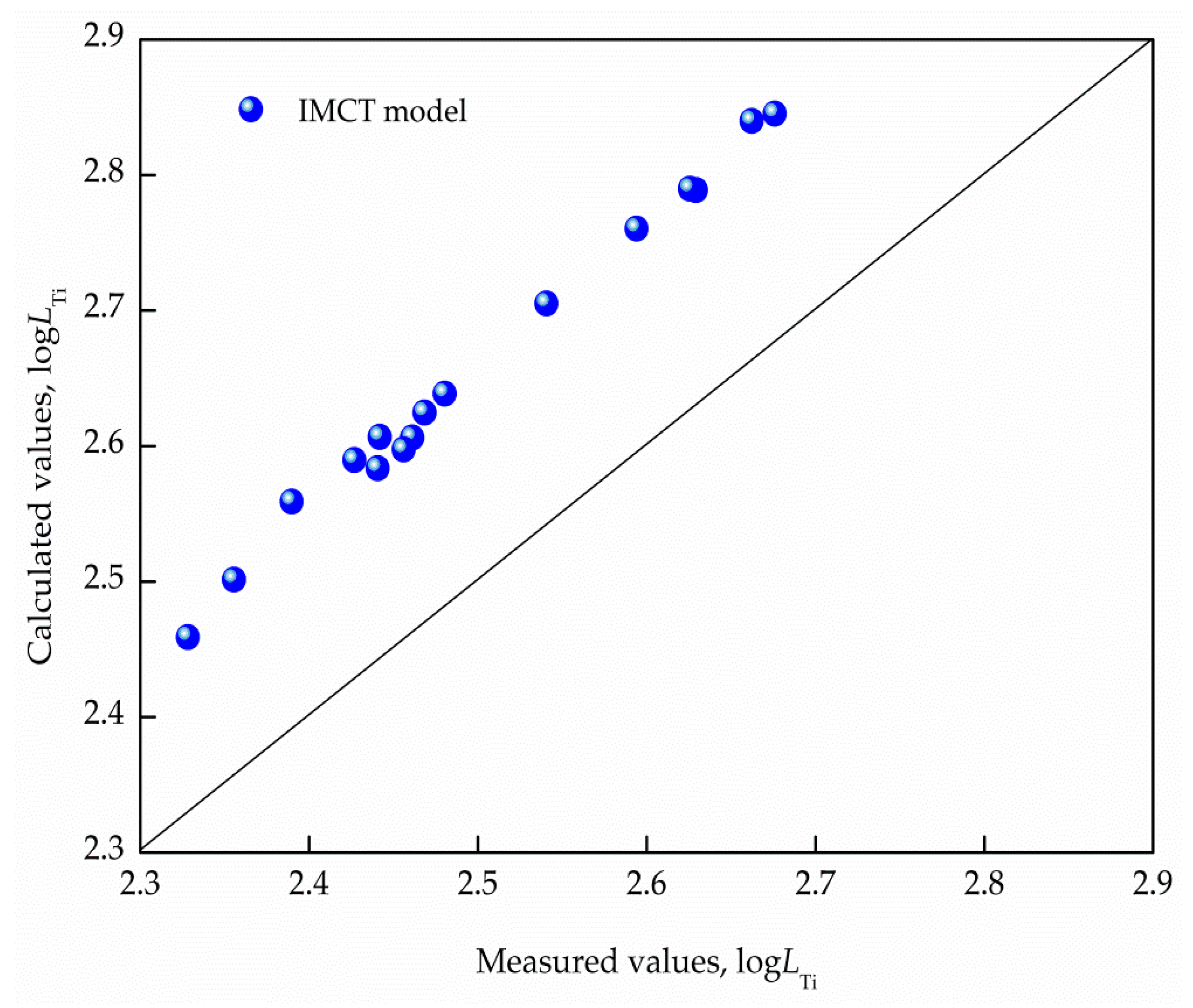
3.1. Comparison of Predicted and Measured Titanium Distribution Ratios

Comparisons between the calculated titanium distribution ratio $L_{\mathrm{Ti},\mathrm{cal}}$ based on the IMCT and the measured $L_{\mathrm{Ti},\mathrm{mea}}$ for CaO–SiO₂–Al₂O₃–MgO–FeO–MnO–TiO₂ slags balanced with liquid steel at 1853 K in the LF process are expounded in Figure 2. It reveals that the titanium distribution ratio predicted by the developed IMCT model exhibited a dependable agreement with the industrially measured results. Moreover, the predicted $L_{\mathrm{Ti},\mathrm{cal}}$ values were all higher than the measured $L_{\mathrm{Ti},\mathrm{mea}}$, which was due to the fact that the calculated values were acquired in an ideal equilibrium state, while during actual industrial production, the slag-metal reaction was in a local equilibrium or quasi-equilibrium state.

To verify the accuracy of the IMCT model, the mean deviations ($\Delta$) of predictions by the IMCT model can be calculated as

$$\Delta =\frac{1}{Z}{\displaystyle \sum }_{n=1}^Z\left|\frac{\log L_{\mathrm{Ti},\mathrm{mea}}-\log L_{\mathrm{Ti},\mathrm{cal}}}{\log L_{\mathrm{Ti},\mathrm{mea}}}\right|\times 100\%=6.29\%<6.3\%$$

(12)

where $L_{\mathrm{Ti},\mathrm{cal}}$ and $L_{\mathrm{Ti},\mathrm{mea}}$ are the calculated and measured titanium distribution ratios, respectively; and Z denotes the number of measured data. The mean deviation was lower than 6.3%, indicating that the titanium distribution ratio model can responsibly predict the maximum de-titanium potential of CaO–SiO₂–Al₂O₃–MgO–FeO–MnO–TiO₂ slags balanced with liquid steel at 1853 K in LF refining, and it can provide guidance for the design of a refining slag system.

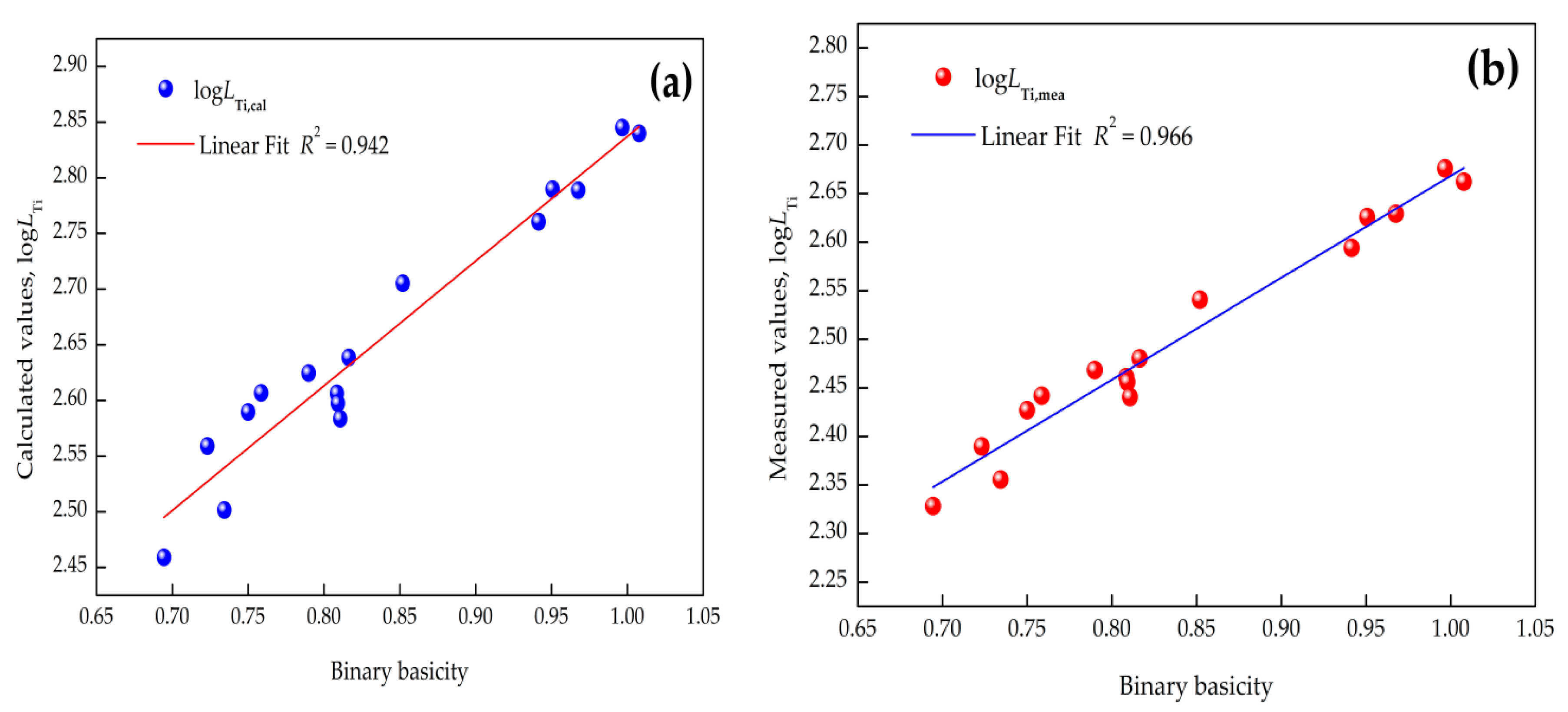
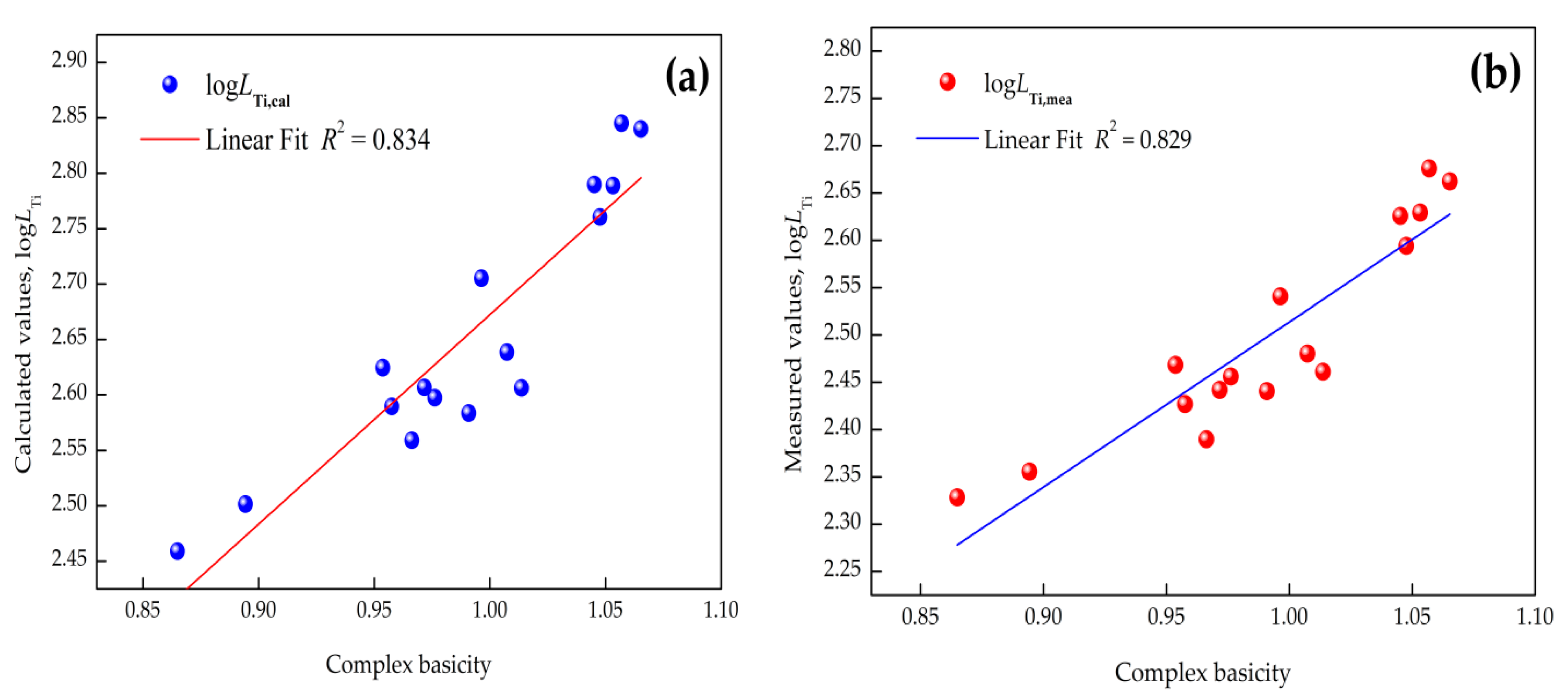
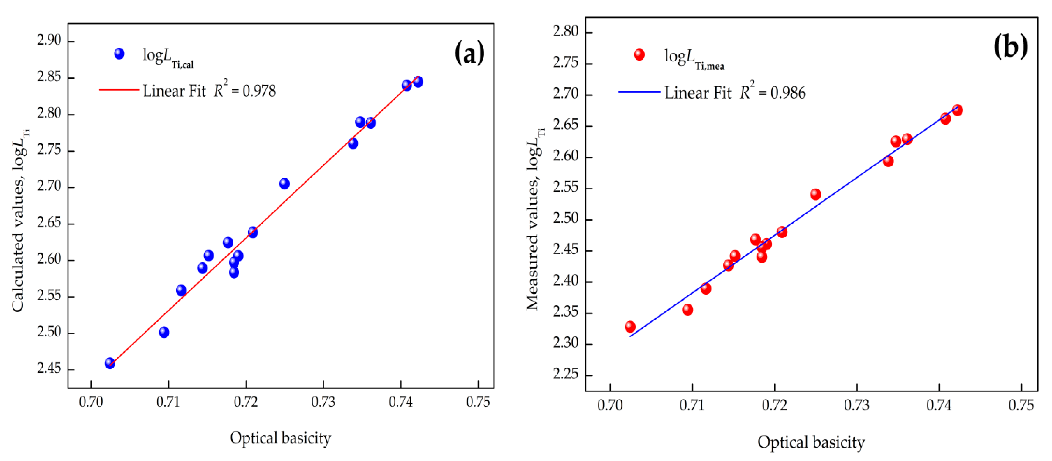
3.2. Influence of Basicity on the Titanium Distribution Ratio

The relation between $L_{\mathrm{Ti},\mathrm{cal}}$ or $L_{\mathrm{Ti},\mathrm{mea}}$ and binary basicity ($\left(\%\mathrm{CaO}\right)/\left({\%\mathrm{SiO}}_2\right)$), complex basicity $\left(\left(\%\mathrm{CaO}\right)+1.4\left(\%\mathrm{MgO}\right)\right)/\left(\left({\%\mathrm{SiO}}_2\right)+\left({\%\mathrm{Al}}_2{\mathrm{O}}_3\right)\right)$, or optical basicity $\Lambda$ ($\Lambda ={\displaystyle \sum }{x}_i·{\lambda }_i$, where $x_i$ is the mole fraction of a component, and ${\lambda }_i$ is the optical basicity of a component in slag) obtained by using Pauling electronegativity [33] are depicted in Figure 3, Figure 4 and Figure 5 (where R is the linear correlation coefficient), respectively. It is evident that (1) the relationship between $\log L_{\mathrm{Ti},\mathrm{cal}}$ by the IMCT model or $\log L_{\mathrm{Ti},\mathrm{mea}}$ and optical basicity had a better dependence than that with the binary or complex basicity of CaO–SiO₂–Al₂O₃–MgO–FeO–MnO–TiO₂ slags and (2) raising the basicity can give rise to a distinctly increasing titanium distribution ratio. Linear fit results indicated that the optical basicity could better reflect the structure of the slags, and it is suggested to reflect the correlation between the titanium distribution ratio and basicity of the slags. The reasons for the different linear fits of these models is attributed to the different definitions of basicity. As for optical basicity, all the components in the slag are taken into account, which can reflect the whole features of the slag, while for binary basicity or complex basicity, the de-titanium contributions of other components were ignored.

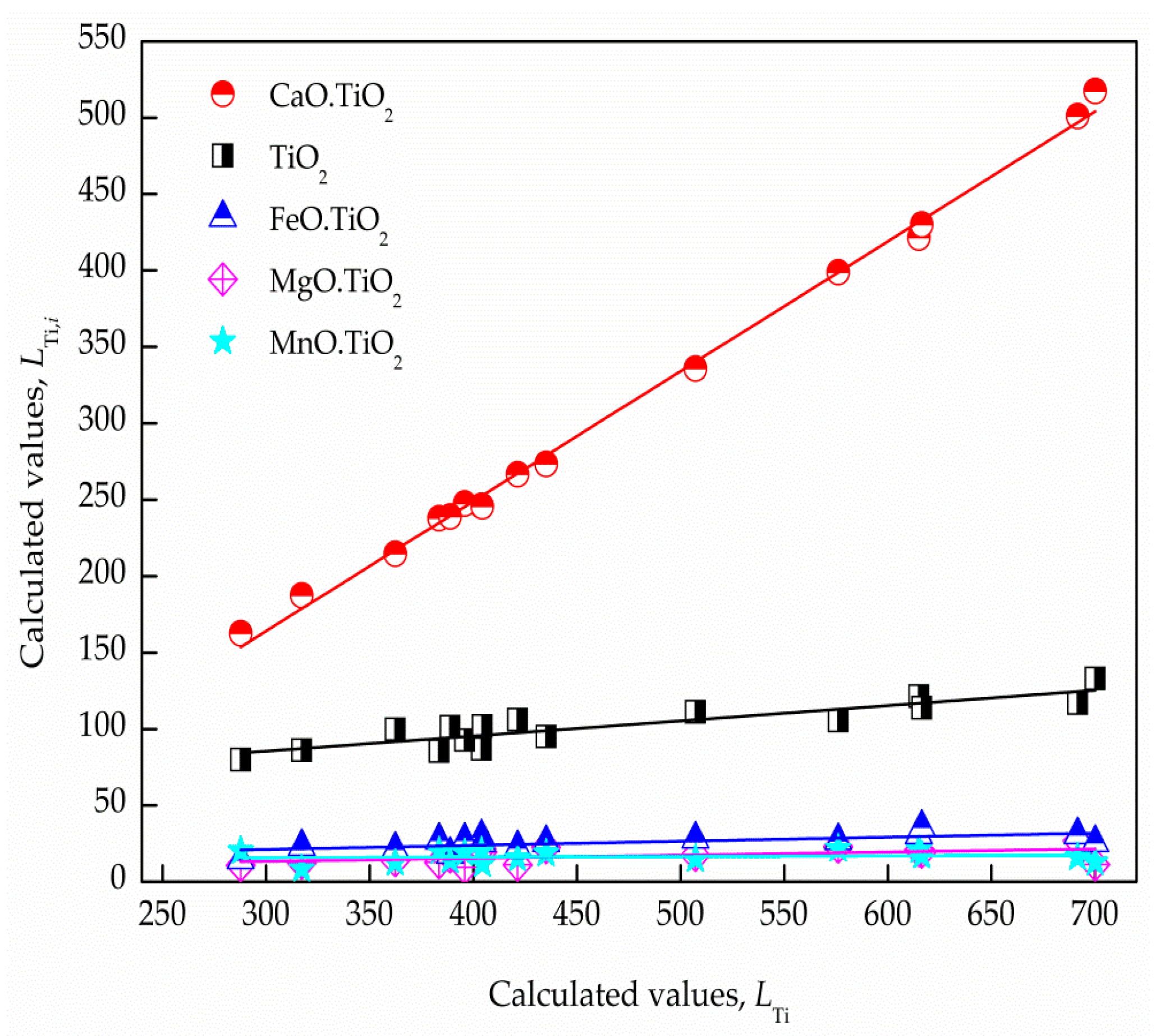
3.3. Contribution Ratio of the Respective Titanium Distribution Ratio Based on the IMCT

In addition to the total titanium distribution ratio of LF refining slags predicted by the established IMCT model, the respective titanium distribution ratio in the present slag system also can be determined. In order to expound the titanium distribution behavior in the LF process, the respective titanium distribution ratios of ${\mathrm{TiO}}_2$, $\mathrm{CaO}·{\mathrm{TiO}}_2$, $\mathrm{MgO}·{\mathrm{TiO}}_2$, $\mathrm{FeO}·{\mathrm{TiO}}_2$, and $\mathrm{MnO}·{\mathrm{TiO}}_2$ in the slags can be acquired by the built IMCT model, respectively, and correlations between the quantitative titanium distribution ratio $L_{\mathrm{Ti},i,\mathrm{cal}}$ of the five structural units and the $L_{\mathrm{Ti},\mathrm{cal}}$ is described in Figure 6. It is evident that $L_{\mathrm{Ti},i,\mathrm{cal}}$ had a nice linear relationship with $L_{\mathrm{Ti},\mathrm{cal}}$, and the respective contribution rates of the structural units containing TiO₂ to total titanium distribution ratios in the slags can be defined by the fitted line gradient.

The regression relationships between $L_{\mathrm{Ti},i,\mathrm{cal}}$ and $L_{\mathrm{Ti},\mathrm{cal}}$ for de-titanium products in the slags are listed in

Table 5. Linear regression expression of $L_{\mathrm{Ti},i,\mathrm{cal}}$ against $L_{\mathrm{Ti},\mathrm{cal}}$ for the structural units containing TiO₂ and their average contribution rates to $L_{\mathrm{Ti},\mathrm{cal}}$ based on IMCT.

Constitutional Units	Expression of ${\mathit{L}}_{\mathbf{T}\mathbf{i},\mathit{i},\mathbf{c}\mathbf{a}\mathbf{l}}\mathbf{against}{\mathit{L}}_{\mathbf{T}\mathbf{i},\mathbf{c}\mathbf{a}\mathbf{l}}$	Average Contribution Rate/%
${\mathrm{TiO}}_2$	$L_{\mathrm{Ti},{\mathrm{TiO}}_2,\mathrm{cal}}=55.5334+0.0997L_{\mathrm{Ti},\mathrm{cal}}$	9.97
$\mathrm{CaO}·{\mathrm{TiO}}_2$	$L_{\mathrm{Ti},\mathrm{CaO}·{\mathrm{TiO}}_2,\mathrm{cal}}=-90.7440+0.8496L_{\mathrm{Ti},\mathrm{cal}}$	84.96
$\mathrm{MgO}·{\mathrm{TiO}}_2$	$L_{\mathrm{Ti},\mathrm{MgO}·{\mathrm{TiO}}_2,\mathrm{cal}}=7.3030+0.0203L_{\mathrm{Ti},\mathrm{cal}}$	2.03
$\mathrm{FeO}·{\mathrm{TiO}}_2$	$L_{\mathrm{Ti},\mathrm{FeO}·{\mathrm{TiO}}_2,\mathrm{cal}}=13.2733+0.0265L_{\mathrm{Ti},\mathrm{cal}}$	2.65
$\mathrm{MnO}·{\mathrm{TiO}}_2$	$L_{\mathrm{Ti},\mathrm{MnO}·{\mathrm{TiO}}_2,\mathrm{cal}}=14.6340+0.0039L_{\mathrm{Ti},\mathrm{cal}}$	0.39

. Table 5 shows that the contribution rates of the five structural units to the predicted $L_{\mathrm{Ti},\mathrm{cal}}$ by the IMCT model were approximately 9.97%, 84.96%, 2.03%, 2.65%, and 0.39%, respectively. It can be concluded from the acquired industrial results that the constitutional unit CaO plays a pivotal role in CaO–SiO₂–Al₂O₃–MgO–FeO–MnO–TiO₂ slags in the de-titanium process.

4. Conclusions

A thermodynamic calculation model for the titanium distribution ratio of CaO–SiO₂–Al₂O₃–MgO–FeO–MnO–TiO₂ slags in the LF process at 1853 K has been established based on the IMCT. The built IMCT model has been tested against industrial measurements. The key findings can be drawn as follows:

(1)

The established IMCT model for calculating the titanium distribution ratio exhibited a dependable agreement with the measurements, and the model can be responsibly applied to predict the maximum de-titanium potential in the LF process at metallurgical temperatures.

(2)

The titanium distribution ratio will increase with the rise of basicity, and the optical basicity is suggested to describe the correlation between basicity and de-titanium ability of the slag. Higher optical basicity is in favor of the de-titanium process.

(3)

The respective titanium distribution ratios of structural units containing TiO₂ can be acquired by the built IMCT model. The contribution rates of ${\mathrm{TiO}}_2$, $\mathrm{CaO}·{\mathrm{TiO}}_2$, $\mathrm{MgO}·{\mathrm{TiO}}_2$, $\mathrm{FeO}·{\mathrm{TiO}}_2$, and $\mathrm{MnO}·{\mathrm{TiO}}_2$ to total de-titanium potential were approximately 9.97%, 84.96%, 2.03%, 2.65%, and 0.39%, respectively, revealing that the structural unit CaO plays a pivotal role in the slags in the de-titanium process.

References

1. Abushosha, R.; Vipond, R.; Mintz, B. Influence of titanium on hot ductility of as cast steels. Mater. Sci. Technol. 1991, 7, 613–621. [Google Scholar] [CrossRef]
2. Chen, Z.; Li, M.; Wang, X.; He, S.; Wang, Q. Mechanism of floater formation in the mold during continuous casting of Ti-stabilized austenitic stainless steels. Metals 2019, 9, 635. [Google Scholar] [CrossRef]
3. Karmakar, A.; Kundu, S.; Roy, S.; Neogy, S.; Srivastava, D.; Chakrabarti, D. Effect of microalloying elements on austenite grain growth in Nb–Ti and Nb–V steels. Mater. Sci. Technol. A 2014, 30, 653–664. [Google Scholar] [CrossRef]
4. Reyes-Calderón, F.; Mejía, I.; Boulaajaj, A.; Cabrera, J.M. Effect of microalloying elements (Nb, V and Ti) on the hot flow behavior of high-Mn austenitic twinning induced plasticity (TWIP) steel. Mater. Sci. Eng. A 2013, 560, 552–560. [Google Scholar] [CrossRef]
5. Cui, H.Z.; Chen, W.Q. Effect of boron on morphology of inclusions in tire cord steel. J. Iron Steel Res. Int. 2012, 19, 22–27. [Google Scholar] [CrossRef]
6. Wu, S.; Liu, Z.; Zhou, X.; Yang, H.; Wang, G. Precipitation behavior of Ti in high strength steels. J. Cent. South Univ. 2017, 24, 2767–2772. [Google Scholar] [CrossRef]
7. Li, J.Y.; Zhang, W.Y. Effect of TiN inclusion on fracture toughness in ultrahigh strength steel. ISIJ Int. 1989, 29, 158–164. [Google Scholar] [CrossRef]
8. Petit, J.; Sarrazin-Baudoux, C.; Lorenzi, F. Fatigue crack propagation in thin wires of ultra high strength steels. Procedia Eng. 2010, 2, 2317–2326. [Google Scholar] [CrossRef] [Green Version]
9. Liu, H.Y.; Wang, H.L.; Li, L.; Zheng, J.Q.; Li, Y.H.; Zeng, X.Y. Investigation of Ti inclusions in wire cord steel. Ironmak. Steelmak. 2011, 38, 53–58. [Google Scholar] [CrossRef]
10. Duan, S.C.; Guo, X.L.; Guo, H.J.; Guo, J. A manganese distribution prediction model for CaO–SiO2–FeO–MgO–MnO–Al2O3 slags based on IMCT. Ironmak. Steelmak. 2017, 44, 168–184. [Google Scholar] [CrossRef]
11. Duan, S.C.; Li, C.; Guo, X.L.; Guo, H.J.; Guo, J.; Yang, W.S. A thermodynamic model for calculating manganese distribution ratio between CaO–SiO2–MgO–FeO–MnO–Al2O3–TiO2–CaF2 ironmaking slags and carbon saturated hot metal based on the IMCT. Ironmak. Steelmak. 2017, 45, 655–664. [Google Scholar] [CrossRef]
12. Li, B.; Li, L.; Guo, H.; Guo, J.; Duan, S.; Sun, W. A phosphorus distribution prediction model for CaO–SiO2–MgO–FeO–Fe2O3–Al2O3–P2O5 slags based on the IMCT. Ironmak. Steelmak. 2019. [Google Scholar] [CrossRef]
13. Yang, X.M.; Li, J.Y.; Chai, G.M.; Duan, D.P.; Zhang, J. A Thermodynamic model for predicting phosphorus partition between CaO–based slags and hot metal during hot metal dephosphorization pretreatment process based on the ion and molecule coexistence theory. Metall. Mater. Trans. B 2016, 47, 2279–2301. [Google Scholar] [CrossRef]
14. Yang, X.M.; Duan, J.P.; Shi, C.B.; Zhang, M.; Zhang, Y.L.; Wang, J.C. A thermodynamic model of phosphorus distribution ratio between CaO–SiO2–MgO–FeO–Fe2O3–MnO–Al2O3–P2O5 slags and molten steel during a top–bottom combined blown converter steelmaking process based on the ion and molecule coexistence theory. Metall. Mater. Trans. B 2011, 42, 738–770. [Google Scholar] [CrossRef]
15. Yang, X.M.; Zhang, M.; Chai, G.M.; Li, J.Y.; Liang, Q.; Zhang, J. Thermodynamic models for predicting dephosphorisation ability and potential of CaO–FeO–Fe2O3–Al2O3–P2O5 slags during secondary refining process of molten steel based on ion and molecule coexistence theory. Ironmak. Steelmak. 2016, 43, 663–687. [Google Scholar] [CrossRef]
16. Li, J.Y.; Zhang, M.; Guo, M.; Yang, X.M. Enrichment mechanism of phosphate in CaO–SiO2–FeO–Fe2O3–P2O5 steelmaking slags. Metall. Mater. Trans. B 2014, 45, 1666–1682. [Google Scholar] [CrossRef]
17. Yang, X.M.; Li, J.Y.; Zhang, M.; Yan, F.J.; Duan, D.P.; Zhang, J. A further evaluation of the coupling relationship between dephosphorization and desulfurization abilities or potentials for CaO–based slags: Influence of slag chemical composition. Metals 2018, 8, 1083. [Google Scholar] [CrossRef]
18. Shi, C.B.; Yang, X.M.; Jiao, J.S.; Li, C.; Guo, H.J. A sulphide capacity prediction model of CaO–SiO2–MgO–Al2O3 ironmaking slags based on the ion and molecule coexistence theory. ISIJ Int. 2010, 50, 1362–1372. [Google Scholar] [CrossRef]
19. Yang, X.M.; Shi, C.B.; Zhang, M.; Chai, G.M.; Wang, F. A thermodynamic model of sulfur distribution ratio between CaO–SiO2–MgO–FeO–MnO–Al2O3 slags and molten steel during LF refining process based on the ion and molecule coexistence theory. Metall. Mater. Trans. B 2011, 42, 1150–1180. [Google Scholar] [CrossRef]
20. Yang, X.M.; Zhang, M.; Shi, C.B.; Chai, G.M.; Zhang, J. A sulfide capacity prediction model of CaO–SiO2–MgO–FeO–MnO–Al2O3 slags during the LF refining process based on the ion and molecule coexistence theory. Metall. Mater. Trans. B 2012, 43, 241–266. [Google Scholar] [CrossRef]
21. Yang, X.M.; Li, J.Y.; Zhang, M.; Chai, G.M.; Zhang, J. Prediction model of sulfide capacity for CaO–FeO–Fe2O3–Al2O3–P2O5 slags in a large variation range of oxygen potential based on the ion and molecule coexistence theory. Metall. Mater. Trans. B 2014, 45, 2118–2137. [Google Scholar] [CrossRef]
22. Yang, X.M.; Li, J.Y.; Zhang, M.; Zhang, J. Prediction model of sulphur distribution ratio between CaO–FeO–Fe2O3–Al2O3–P2O5 slags and liquid iron over large variation range of oxygen potential during secondary refining process of molten steel based on ion and molecule coexistence theory. Ironmak. Steelmak. 2016, 43, 39–55. [Google Scholar] [CrossRef]
23. Yang, X.M.; Zhang, M.; Zhang, J.L.; Li, P.C.; Li, J.Y.; Zhang, J. Representation of oxidation ability for metallurgical slags based on the ion and molecule coexistence theory. Steel Res. Int. 2014, 85, 347–375. [Google Scholar] [CrossRef]
24. Verein Deutscher Eisenhuttenleute (VDEh). Slag Atlas, 2nd ed.; Woodhead Publishing Limited: Cambridge, UK, 1995. [Google Scholar]
25. Chen, J.X. Common Charts and Databook for Steelmaking, 2nd ed.; Metallurgical Industry Press: Beijing, China, 2010. [Google Scholar]
26. Zhang, J. Computational Thermodynamics of Metallurgical Melts and Solutions; Metallurgical Industry Press: Beijing, China, 2007. [Google Scholar]
27. Rein, R.H.; Chipman, J. Activities in the liquid solution SiO2–CaO–MgO–Al2O3 at 1600 °C. Trans. Met. Soc. AIME 1965, 233, 415–425. [Google Scholar]
28. Turkdogan, E.T. Physical Chemistry of High Temperature Technology; Academic Press: New York, NY, USA, 1980; pp. 8–12. [Google Scholar]
29. Gaye, H.; Welfringer, J. Proceedings of the Second International Symposium on Metallurgical Slags and Fluxes; Fine, H.A., Gaskell, D.R., Eds.; TMS–AIME: Lake Tahoe, NV, USA, 1984; pp. 357–375. [Google Scholar]
30. Ban-ya, S.; Chiba, A.; Hikosaka, A. Thermodynamics of FetO–MxOy(MxOy=CaO, SiO2, TiO2, and Al2O3) binary melts in equilibrium with solid iron. Tetsu-To-Hagane 1980, 66, 1484–1493. [Google Scholar] [CrossRef]
31. Timucin, M.; Muan, A. Activity–composition relations in NiAl2O4–MnAl2O4 solid solutions and stabilities of NiAl2O4 and MnAl2O4 at 1300 °C and 1400 °C. J. Am. Ceram. Soc. 1992, 75, 1399–1406. [Google Scholar] [CrossRef]
32. Barin, I.; Knacke, O.; Kubaschewski, O. Thermochemical Properties of Inorganic Substances (Supplement); Springer: New York, NY, USA, 1977; pp. 392–445. [Google Scholar]
33. Pauling, L. The Nature of Chemical Bond; Cornell University Press: Ithaca, NY, USA, 1960. [Google Scholar]
Figure 1. Production process of high-strength tire cord steel.
Processes 07 00788 g001
Figure 2. Comparisons between measured and calculated titanium distribution ratios for CaO–SiO2–Al2O3–MgO–FeO–MnO–TiO2 slags.
Processes 07 00788 g002
Figure 3. Correlation between binary basicity and titanium distribution ratio: (a) calculated by IMCT; (b) industrial measurements.
Processes 07 00788 g003
Figure 4. Correlation between complex basicity and titanium distribution ratio: (a) calculated by IMCT; (b) industrial measurements.
Processes 07 00788 g004
Figure 5. Correlation between optical basicity and titanium distribution ratio: (a) calculated by IMCT; (b) industrial measurements.
Processes 07 00788 g005
Figure 6. Correlation between the respective titanium distribution ratio and the total titanium distribution ratio of the slags, the solid line of color red, black, blue, magenta, and cyan represent the contribution ratio of CaO∙TiO2, TiO2, FeO∙TiO2, MgO∙TiO2, and MnO∙TiO2, respectively.
Processes 07 00788 g006