Formation Mechanism of Trailing Oil in Product Oil Pipeline

Abstract
: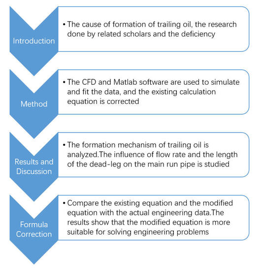
1. Introduction
2. Method
3. Model
4. Simulation Results and Discussion
4.1. Analysis of the Mechanism of Dead-Leg Mixing
4.2. The Influence of Velocity on the Trailing Oil
4.3. The Effect of the Dead-Leg Length on Trailing Oil
5. Formula Correction
6. Conclusions
Author Contributions
Funding
Conflicts of Interest
References
- Liu, L.; Han, X. Contaminated products in batch transportation pipeline of finished products and their treatment. Pet. Geol. Eng. 2005, 19, 68–69. [Google Scholar]
- Cafaro, V.G.; Pautasso, P.C.; Cerdá, J.; Cafaro, D.C. Efficient planning of crude oil supplies through long-distance pipelines. Comput. Chem. Eng. 2018, 1–15. [Google Scholar] [CrossRef]
- Shin, J.O.; Balziel, S.B.; Linden, P.F. Gravity Currents Produced by Lock Exchange. J. Fluid Mech. 2004, 521, 1–34. [Google Scholar] [CrossRef]
- Parfomak, P.W.; Nerurkar, N.; Luther, L.; Burrows, V.K. Keystone XL Pipeline Project: Key Issues. Congressional Research Service; Congressional Research Service: Washington, DC, USA, 2011. [Google Scholar]
- Levenspiel, O. How much mixing occurs between batches? Pipe Line Ind. 1958, 24, 51–54. [Google Scholar]
- Taylor, G. Dispersion of Soluble Matter in Solvent Flowing Slowly through a Tube. Proc. Math. Phys. Eng. Sci. 1953, 219, 186–203. [Google Scholar] [CrossRef]
- Aunicky, A. The longitudinal mixing of liquids flowing successively in pipelines. Can. J. Chem. Eng. 1970, 48, 12–16. [Google Scholar] [CrossRef]
- Krantz, W.B.; Wasan, D.T. Axial Dispersion in the Turbulent Flow of Power-Law Fluids in Straight Tubes. Ind. Eng. Chem. Fundam. 1974, 13, 56–62. [Google Scholar] [CrossRef]
- Austin, J.E.; Palfrey, J.R. Mixing of Miscible but Dissimilar Liquids in Serial Flow in a Pipeline. Proc. Instn. Mech. Engrs. 1963, 178, 377–395. [Google Scholar] [CrossRef]
- Scott, D.S.; Dullien, F.A.L. Diffusion of ideal gases in capillaries and porous solids. AIChE J. 1962, 8, 113–117. [Google Scholar] [CrossRef]
- Levenspiel, O. Longitudinal Mixing of Fluids Flowing in Circular Pipes. Ind. Eng. Chem. 1958, 50, 343–346. [Google Scholar] [CrossRef]
- Deng, S.; Pu, J. Application of convection-diffusion equation to the analyses of contamination between batches in multi-products pipeline transport. Appl. Math. Mech. 1998, 19, 757–764. [Google Scholar] [CrossRef]
- Botros, K.K. Estimating contamination between batches in products lines. Oil Gas J. 1984, 82, 112–114. [Google Scholar]
- Rachid, F.B.D.F.; Araujo, J.H.C.D.; Baptista, R.M. The Influence of Pipeline Diameter Variation on the Mixing Volume in Batch Transfers. In Proceedings of the 2002 4th International Pipeline Conference, Calgary, AB, Canada, 29 September–3 October 2002; pp. 997–1004. [Google Scholar] [CrossRef]
- Rachid, F.B.F.; Araujo, J.H.C.D.; Baptista, R.M. Predicting Mixing Volumes in Serial Transport in Pipelines. J. Fluids Eng. Trans. Asme 2002, 124, 528–534. [Google Scholar] [CrossRef]
- Patrachari, A.R.; Johannes, A.H. A conceptual framework to model interfacial contamination in multiproduct petroleum pipelines. Int. J. Heat Mass Transf. 2012, 55, 4613–4620. [Google Scholar] [CrossRef]
- Botros, K.K.; Clavelle, E.J.; Vogt, G.M. Interfacial Contamination Between Batches of Crude Oil to Dead-Legs in Pump Station Piping. J. Energy Resour. Technol. 2016, 138, 1–8. [Google Scholar] [CrossRef]
- Jamalabadi, M.Y.A.; DaqiqShirazi, M.; Kosar, A.; Shadloo, M.S. Effect of injection angle, density ratio, and viscosity on droplet formation in a microfluidic T-junction. Theor. Appl. Mech. Lett. 2017, 7, 243–251. [Google Scholar] [CrossRef]
- Li, X. Calculation method for length of oil mixtures in product pipelines. Oil Gas Storage Transp. 2015, 34, 497–499. [Google Scholar] [CrossRef]
- Chen, Q. Calculations on the Mixing Volume of Products Pipeline with Variable Diameter Pipes. Oil Gas Storage Transp. 1999, 18, 7–8. [Google Scholar]
- Neutrium. Calculating Interface Volumes for Multi-Product Pipelines. Available online: https://neutrium.net/fluid_flow/calculating-interface-volumes-for-multi-product-pipelines/ (accessed on 1 December 2018).
- De Arauro, J.H.C.; Gomes, P.D.; Ruas, V. Study of a finite element method for the time-dependent generalized Stokes system associated with viscoelastic flow. J. Comput. Appl. Math. 2010, 234, 2562–2577. [Google Scholar] [CrossRef]
- Liu, E.; Lv, L.; Ma, Q.; Kuang, J.; Zhang, L. Steady-state optimization operation of the West-East Gas Pipeline. Adv. Mech. Eng. 2019, 11, 1–14. [Google Scholar] [CrossRef]
- Menter, F.; Egorov, Y. The Scale-Adaptive Simulation Method for Unsteady Turbulent Flow Predictions. Part 1: Theory and Model Description. Appl. Sci. Res. 2010, 85, 113–138. [Google Scholar] [CrossRef]
- Liu, E.; Yan, K.; Peng, B. Noise silencing technology for manifold flow noise based on ANSYS fluent. J. Nat. Gas Sci. Eng. 2016, 29, 322–328. [Google Scholar] [CrossRef]
- Liu, E.; Tan, H.; Peng, S. A CFD simulation for the ultrasonic flow meter with a header. The. Vjesn. 2017, 24, 1797–1801. [Google Scholar] [CrossRef]
- Liu, E.; Peng, S.; Yang, T. Noise silencing technology for upright venting pipe jet noise. Adv. Mech. Eng. 2018, 10, 1–15. [Google Scholar] [CrossRef]
- Pan, Z.; Chen, B.; Shang, L. Numerical Simulation of V-cone Flow Meter in Product Oil Pipeline of Batch Transportation. Pet. Sci. Technol. 2010, 28, 925–933. [Google Scholar] [CrossRef]
- Lebon, B.; Nguyen, M.Q.; Peixinho, J.; Shadloo, M.S.; Hadjadj, A. A new mechanism for periodic bursting of the recirculation region in the flow through a sudden expansion in a circular pipe. Phys. Fluids 2018, 30, 1–5. [Google Scholar] [CrossRef]
- Jiang, L.; Wang, S.; Zhang, Z.; Guo, Q.; Xu, Y. Effects of mixed oil tailing of products pipeline on cutting concentration. Oil Gas Storage Transp. 2014, 33, 848–851. [Google Scholar] [CrossRef]
- Yuan, Q.; Wu, C.; Yu, B.; Han, D.; Zhang, X.; Cai, L.; Sun, D. Study on the thermal characteristics of crude oil batch pipelining with differential outlet temperature and inconstant flow rate. J. Pet. Sci. Eng. 2018, 160, 519–530. [Google Scholar] [CrossRef]
- Yong, C.; Xu, P.; Hao, Y. Mechanical performance experiments on rock and cement, casing residual stress evaluation in the thermal recovery well based on thermal-structure coupling. Energy Explor. Exploit. 2017, 35, 591–608. [Google Scholar] [CrossRef]
- Wang, Z.; Fu, X.; Ping, G.; Tu, H.; Wang, H.; Zhong, S. Gas-liquid flowing process in a horizontal well with premature liquid loading. J. Nat. Gas. Sci. Eng. 2015, 25, 207–214. [Google Scholar] [CrossRef]
- Wang, Z.; Tu, H.; Guo, P.; Zeng, F.; Sang, T.; Wang, Z. Fluid behavior of gas condensate system with water vapor. Fluid Phase Equilibria 2017, 438, 67–75. [Google Scholar] [CrossRef]


| Preceding Batch | Following Batch | |
|---|---|---|
| Physical property | 92# | 0# |
| Density (kg/m3) | 724 | 842 |
| Viscosity (10−6 m2/s) (20 °C) | 0.404 | 5.069 |
| Grid Quantity | 603,042 | 1,532,450 | 2,034,860 | 3,021,580 |
| Oil Volume Fraction | 0.188 | 0.186 | 0.192 | 0.188 |
| Relative Error | 1.06% | 3.13% | 2.08% | |
| Time Step (s) | 0.0005 | 0.001 | 0.005 | 0.01 |
| Oil Volume Fraction | 0.19 | 0.188 | 0.32 | 0.48 |
| Relative Error | 1.05% | 41.25% | 33.33% |
| Time (s) | Velocity (m/s) | Length of Dead-Leg (m) |
|---|---|---|
| 421 | 0.4 | 3.19 |
| 468 | 0.6 | 3.37 |
| 441 | 0.61 | 3 |
| 501 | 0.8 | 3.49 |
| 562 | 1.0 | 3.68 |
| 603 | 1.2 | 3.8 |
| 672 | 1.4 | 3.99 |
| 720 | 1.6 | 4.1 |
| 920 | 1.8 | 4.52 |
| 979 | 1.86 | 5 |
| 1324 | 2.0 | 5.14 |
| 2248 | 3.19 | 6 |
| 4186 | 4.18 | 7 |
| Number of Dead-Legs | Average Density of Contamination (kg/m3) | Oil Substitution Time in Dead-Leg (s) | Trailing Oil Length (m) |
|---|---|---|---|
| 1 | 832 | 672 | 136 |
| 2 | 820 | 690 | 148 |
| 3 | 810 | 705 | 158 |
| 4 | 802 | 717 | 166 |
| 5 | 795 | 727 | 173 |
| 6 | 789 | 735 | 179 |
| 7 | 784 | 742 | 185 |
| 8 | 781 | 749 | 190 |
| 9 | 779 | 754 | 195 |
| 10 | 778 | 758 | 200 |
| 11 | 777 | 760 | 201 |
| 12 | 777 | 762 | 202 |
© 2018 by the authors. Licensee MDPI, Basel, Switzerland. This article is an open access article distributed under the terms and conditions of the Creative Commons Attribution (CC BY) license (http://creativecommons.org/licenses/by/4.0/).
Share and Cite
Liu, E.; Li, W.; Cai, H.; Peng, S. Formation Mechanism of Trailing Oil in Product Oil Pipeline. Processes 2019, 7, 7. https://doi.org/10.3390/pr7010007
Liu E, Li W, Cai H, Peng S. Formation Mechanism of Trailing Oil in Product Oil Pipeline. Processes. 2019; 7(1):7. https://doi.org/10.3390/pr7010007
Chicago/Turabian StyleLiu, Enbin, Wensheng Li, Hongjun Cai, and Shanbi Peng. 2019. "Formation Mechanism of Trailing Oil in Product Oil Pipeline" Processes 7, no. 1: 7. https://doi.org/10.3390/pr7010007