Numerical Investigation of Hydraulic Fracture Propagation Based on Cohesive Zone Model in Naturally Fractured Formations

Abstract

Complex propagation patterns of hydraulic fractures often play important roles in naturally fractured formations due to complex mechanisms. Therefore, understanding propagation patterns and the geometry of fractures is essential for hydraulic fracturing design. In this work, a seepage–stress–damage coupled model based on the finite pore pressure cohesive zone (PPCZ) method was developed to investigate hydraulic fracture propagation behavior in a naturally fractured reservoir. Compared with the traditional finite element method, the coupled model with global insertion cohesive elements realizes arbitrary propagation of fluid-driven fractures. Numerical simulations of multiple-cluster hydraulic fracturing were carried out to investigate the sensitivities of a multitude of parameters. The results reveal that stress interference from multiple-clusters is responsible for serious suppression and diversion of the fracture network. A lower stress difference benefits the fracture network and helps open natural fractures. By comparing the mechanism of fluid injection, the maximal fracture network can be achieved with various injection rates and viscosities at different fracturing stages. Cluster parameters, including the number of clusters and their spacing, were optimal, satisfying the requirement of creating a large fracture network. These results offer new insights into the propagation pattern of fluid driven fractures and should act as a guide for multiple-cluster hydraulic fracturing, which can help increase the hydraulic fracture volume in naturally fractured reservoirs.

1. Introduction

Hydraulic fracturing is an evolving technology that has been used to increase oil recovery in naturally fractured reservoirs [1]. The widely held assumption that hydraulic fractures in these reservoirs are ideal, simple, straight, bi-wing, planar features is not accurate because of stress shadows and the existence of pre-existing natural fractures (NFs) [2]. Multiple-cluster hydraulic fracturing of horizontal wells is a commonly used method in ultra-low permeability and massive natural fracture reservoirs. This technique aims to widen hydraulic fractures (HFs) and generate a large amount of non-planar hydraulic fracture networks (HFNs) [3]. Thus, an accurate mechanism of NF–HF interaction needs to be provided, which ultimately determines the stimulated reservoir volume (SRV) and production.

Various complex fracturing models of naturally fractured formations have been developed to describe the complex interaction mechanism between NFs and HFs, such as the boundary element method (BEM) [1,2,3], discrete element method (DEM) [4,5,6,7,8], and the finite element method (FEM) based on the cohesive zone method (CZM). Such models intend to overcome the limitations of conventional hydraulic fracturing models, in which HFs are simulated to be planar and bi-wings.

Olson et al. [3,9] proposed a numerical code based on a pseudo-3D displacement discontinuity solution, which provided a preliminary analysis of a complex fracture network with a constant pressure boundary condition. This method, however, could not offer a solution for flow patterns within the fracture network. Zhang et al. [1] developed a BEM program coupling rock deformation and a fluid flow hydraulic fracturing model for a fracture network, which considered multi-fracture propagation and interactions between HFs and NFs. Kan et al. [10] made an improvement to describe the complexities of a HFN, in which the natural fracture could be modeled with many connected linear elements with uniform openings and shearing displacement discontinuities. The disadvantages of the three aforementioned models, including BEM or the displacement discontinuity method, are as follows: they do not achieve an efficient and accurate fracture propagation and do not address the limitations in the mesh shape. Further, discretization for the body boundaries only may lead to serious computation problems and make it challenging to find an iteration solution for unknown boundaries.

The discrete element method (DEM) has been used in modeling hydraulic fracturing networks, in which the generation of HFs can be achieved by a flow network consisting of bond particles or deformable blocks. Hamidi et al. [4] presented a three-dimensional distinct element code (3DEC) to simulate the initiation and propagation of hydraulic fractures induced by hydro-mechanics in a typical fractured formation. Nevertheless, the discrete element method could not be used to model fracture initiation in an intact rock matrix. Therefore, a set of joints were introduced in this method for simulating this process. Zhang et al. [11] used a mixed finite element and discrete element method to develop a model for predicting the initiation and propagation of hydraulic fractures in tight gas reservoirs. As a consequence, a newly complex fracturing model based on a 3D discrete element method was introduced into the naturally fractured formation with multi-layers to simulate the propagation and interaction between hydraulic fracture networks [6,8]. However, the complex fracture network model based on DEM needs a small time increment, which makes it difficult for computation [12].

A representative numerical method for modeling hydraulic fractures is the finite element method based on the CZM, which considers the effects of the fracture tip process zone and softening. Owing to the advantages of the CZM, a finite model based on the CZM was used to simulate full coupling between the incompressible viscous fluid and rock matrix, which was demonstrated to be relatively accurate in hydraulic fracturing under plain strain conditions [13,14,15,16]. For the strong non-linear coupling in the hydraulic fracturing process, empirical methods and the linear elastic method, which ignore the effects of the plastic zone and softening, still occupy an important position for design and optimization of hydraulic fracture schemes. However, the CZM model, in the framework of non- linear elastic fracture mechanics provided by Haddad et al. [17], can easily solve this problem. Guo et al. [18,19] used a new model based on the CZM coupled with the seepage-damage field for simulating the interaction between HFs and NFs; multi-layers in the formation were also investigated using this model. The results revealed that the model is highly accurate in predicting fracture initiation and propagation. Moreover, the intersections between HFs and NFs were also in strong agreement with the experimental exercise and analytical solution. Li et al. [12] presented a new pore pressure cohesive element that applied Coulomb’s frictional contact model to detail the fracture contact behavior for modeling HFN. In general, the finite element method based on the CZM has significant advantages that make it suitable for modeling the hydraulic fracture process, including fracture tip evolution and a softening effect. Further, the numerical model developed by the CZM is computed using an implicit integration with fewer calculation problems than the dis-continuum method, which uses an explicit integration scheme with a small time increment.

In this study, a fully coupled seepage–stress model based on ABAQUS is developed to simulate the propagation of HFs in naturally fractured reservoirs. Two types of elements—the plain strain element coupling pore fluid stress, and pore pressure cohesive element—are applied to model the rock matrix and fractures, respectively. The zero-thickness pore pressure cohesive zone (PPCZ) elements are incorporated into the finite element model using a python code written by the authors, in which two neighboring quadrangle elements are inserted into one PPCZ element. Different constructions of multiple-cluster hydraulic fracturing are developed to investigate complex propagation pattern between HFs and NFs. Furthermore, various parameters including stress difference, cluster spacing, injection fluid viscosity, and numbers of clusters are investigated for a typical field case. The effect of different parameters on the fracture network are captured with different stress states. The optimal parameters of the fracturing process are determined, and the propagation pattern including NFs and HFs is predicted.

2. Governing Equations

Owing to a modification of the CZM, the latest efforts to model hydraulic fracturing based on ABAQUS have introduced the pore pressure node in cohesive elements since ABAQUS 6.12 [14,15,16,17,20,21]. Further, the presence of joint pore pressure nodes among intersection pore pressure cohesive elements makes it possible to model the intersection of fractures. In this model, gradual damage occurs at the intersection of pore pressure nodes, which leads to arbitrary propagation during the fracturing process. Moreover, hydraulic fracturing coupling in situ stress and pore pressure can be solved by the geo-mechanics model with geostatic and soil analyses in standard analysis. Therefore, the results of fully-coupled pore pressure stress can be achieved easily by including the linear and nonlinear material effects and fluid leak-off between cohesive layers and bulk rocks.

2.1. Fluid Flow within the CZM

The fracturing fluid within the CZM model is hypothesized to be an incompressible Newtown fluid governed by the lubrication equation [22]. As shown in Figure 1, both normal and tangential flow can be simulated with the cohesive elements. The shale matrix is considered to be comprised of pore pressure materials, in which fluid loss into the matrix is also taken into account to approximate the field application. Therefore, the global volume balance equation for tangential flow that was formulated by Poiseuille was applied:

$$q=-\frac{w^3}{12\mu }\nabla p_f$$

(1)

where q is the fluid volume crossing though the cohesive gap, w is the fracture width, μ is the viscosity of the fracturing fluid, and $\nabla p_f$ is the gradient of pressure along the cohesive zone. This equation assumes that the injection rate is proportional to both the pressure gradient and the cube of the fracture width and inversely proportional to the fracturing fluid viscosity.

The normal flow represents the permeation of fracturing fluid by proposing two permeable cohesive layers, in which leak-off coefficients for the two cohesive layers are taken into consideration, as shown in Figure 2. The normal flow is formulated as

$$\begin{array}{l}{q}_t=c_t(p_i-p_t)\\ q_b=c_b(p_i-p_b)\end{array}$$

(2)

where $q_t$ and $q_b$ are the volumes of permeation for the up and side surfaces, respectively; $c_t$ and $c_b$ are the leak-off coefficients for the top and bottom cohesive layers, respectively; $p_t$ and $p_b$ are the pore pressures on the top and bottom surfaces, respectively; and $p_i$ is the pore pressure in the middle of the cohesive element gap.

For a specific time, the injection fluid flows into the fracture when the cohesive layer fails completely. Injection fluid flows into the fracture, with the tangential flow along the fracture direction and normal flow leak-off into the surrounding formations. The continuity equation of the fracture fluid can be expressed as

$$\frac{\partial w}{\partial t}+\nabla q+(q_t+q_b)=\mathrm{Q}\left(\mathrm{t}\right)\delta (\mathrm{x},\mathrm{y})$$

(3)

where q is the tangential flow mass and Q is the total volume of injection fluid.

2.2. Damage Initiation and Evolution of Cohesive Elements

In this study fluid flow in the fracture network, seepage in a porous media, and the elastic deformation of a rock matrix are fully coupled in the cohesive zone model, unlike the bulk-continuum materials which describe continuum behaviors with stress and strain. The cohesive method uses the traction and separation law for the interface. In the fully coupled model, Biot’s [23] effective stress principle is adopted to describe the effective stress due to the rock skeleton and pore pressure. The principle of effective stress is formulated below:

$${\sigma }_{ij}={\sigma }_{ij}^{\prime }+\alpha p{\delta }_{ij}$$

(4)

where ${\sigma }_{ij}$ is the total stress, ${\sigma }_{ij}^{\prime }$ is the effective stress, α is the Biot constant, p is the pore pressure, and ${\delta }_{ij}$ is the tensor of Kronecker.

The traction–separation damage can be divided into three stages: Initial loading before damage, damage initiation, and damage evolution. The corresponding traction–separation stress vector and stiffness matrix are introduced to find a solution, which can be expressed as:

$$\overrightarrow{t}=\{\begin{array}{l}{t}_s\\ t_n\\ t_t\end{array}\}=\left[\begin{array}{l}\begin{array}{ccc}{K}_{nn}& K_{ns}& K_{nt}\end{array}\\ \begin{array}{ccc}{K}_{ns}& K_{ss}& K_{st}\end{array}\\ \begin{array}{ccc}{K}_{nt}& K_{st}& K_{tt}\end{array}\end{array}\right]\{\begin{array}{c}{\epsilon }_n\\ {\epsilon }_s\\ {\epsilon }_t\end{array}\}=\left(\frac{1}{T^{coh}}\right)\overrightarrow{K}\overrightarrow{\delta }$$

(5)

where $\overrightarrow{t}$ is the traction stress vector on the cohesive element layer, $\overrightarrow{\delta }$ represents the interface separation, $T^{coh}$ is the cohesive element initial gap that is used to calculate the element stiffness, K is the element stiffness, and ε is the strain vector.

In this model, typical zero thickness cohesive elements are embedded in the pore pressure element for modeling an arbitrary propagation of fractures. For the fracture initiation, we used the quadratic nominal stress law to combine the mixed model failure. Damage initiates when the quadratic interaction function reaches a value of one, which involves one normal and two shear nominal stresses. The initiating behavior is shown in Figure 3 and summarized in the function

$${\left(\frac{\langle t_n\rangle }{t_n^0}\right)}^2+{\left(\frac{t_s}{t_s^0}\right)}^2+{\left(\frac{t_t}{t_t^0}\right)}^2=1$$

(6)

The metric for damage is a stiffness degradation index, D, which represents the entire damage caused by all stress components. In particular, no damage occurs (D = 0) at the beginning of the simulation, and the cohesive element also satisfies the condition under pure compressive stress. In addition, full degradation of the cohesive element occurs at all integration points when D = 1, which means a zero load carrying capacity for these elements.

$$t_n=\{\begin{array}{cc}(1-D)T_n,& T_n\ge 0\\ T_n,& T_n<0\end{array}$$

(7)

$$t_s=(1-D)T_s,$$

(8)

$$t_t=(1-D)T_t,$$

(9)

where T_n, T_s and T_t are the normal and shear stress components predicted by the elastic traction–separation behavior for current separation without damage.

Nevertheless, the behavior of D depends on the nature of material softening, which could be linear and exponential. The index is a function of the effective relative displacement, δ_m, that accounts for combining the effects of δ_n, δ_s and δ_t:

$${\delta }_m=\sqrt{{\langle {\delta }_n\rangle }^2+{\delta }_s{}^2+{\delta }_t{}^2}$$

(10)

For this particular model, linear softening behavior is represented as

$$D=\frac{{\delta }_m^f({\delta }_m^{\max }-{\delta }_m^0)}{{\delta }_m^{\max }({\delta }_m^f-{\delta }_m^0)}$$

(11)

where δ_m is the relative effective displacement attained over the course of loading. The superscripts max, f and 0 represent the max relative displacement, displacement when fractures are completely damaged, and the displacement at damage initiation, respectively.

Once fracture initiation occurs, damage can be evaluated using fracture energy theory. The Benzeggagh–Kenane criterion is introduced to model the fracture process. Figure 4 shows the schematic of the mix-mode Benzeggagh–Kenane (BK) criterion during fracture evolution. Moreover, the corresponding formulas of the mechanic criteria can be expressed as

$$G_n^c+(G_s^c-G_n^c){\left(\frac{G_s+G_t}{G_n+G_s+G_t}\right)}^{\eta }=G^c$$

(12)

where G represents the energy release rate. Superscript c is the critical energy release rate. The subscripts n, s, and t denote the directions of the normal stress and the two shear stresses, and η is a constant for a corresponding material property. The symbol $\langle \rangle$ is the Macaulay bracket. For a negative t, the value in the Macaulay bracket would be zero, which means that the cohesive element has an incompressible property.

2.3. Equilibrium Equation

In the simulation, the formation is assumed to be a porous medium corresponding to the field rock matrix. Only a single phase of fluid is saturated into the solid skeleton and pores. The total stress within the formation consists of two parts: The total effective stress $\overline{\sigma }$ is determined by the skeleton and the pore pressure p_w. According to the principle of virtual work, the finite element method equilibrium equation can be formulated as

$${\displaystyle \int \left(\overline{\sigma }-p_{w}I\right)}\delta \epsilon dV={\displaystyle {\int }_{S}t\cdot \delta }vdS+{\displaystyle {\int }_{V}f\cdot \delta vdV}$$

(13)

where $\overline{\sigma }$ and p_w are the Boit effective stress and pore pressure, respectively; $\delta \epsilon$ and $\delta v$ are the virtual strain rate and virtual velocity, respectively; t and f are the surface displacement per unit area and body force per unit volume, repectively; and I is the unit matrix.

Fluid flow is required in a porous media according to the continuum equation. The change in total fluid mass is equal to the fluid mass crossing the cohesive surface per unit time. Moreover, fluid flow in a porous medium follows Darcy’s law. The continuum equation for fluid leak-off can be derived as follows:

$$\frac{1}{J}\frac{\partial }{\partial t}\left(J{\rho }_w{n}_w\right)+\frac{\partial }{\partial x}\cdot \left({\rho }_w{n}_w{v}_w\right)=0$$

(14)

where J is the volume change ration; ${\rho }_w$, $n_w$ and $v_w$ are the mass density of liquid, porosity of medium and average velocity of liquid relative to the solid phase, respectively; and x is the space vector.

3. Results and Discussion

The two-dimensional symmetrical models were used to model the stratum for multiple-cluster hydraulic fracturing, which extended for 200 m in the direction of horizontal minimal stress (X direction), and for 100 m in the direction of maximal stress (Y direction). There were three types of perforations (two, three and four clusters) with single stage perforations. Each configuration had a distance spacing of 30 m, 40 m, 50 m and 60 m. The natural fractures were designed for an approaching angle of 60° with random lengths of 4–6 m, as shown in Figure 5. However, hydraulic fracturing is a complex nonlinear problem that is coupled with several factors; thus, the viscosity control parameter of a cohesive element was introduced to guarantee convergence. In this work, the viscosity parameter was restricted to 0.01, and its value was verified by the 2016 ABAQUS user′s manual. To prevent the mesh size from having an effect, the normal global mesh size was set as 1 m, which can result in fine propagation of fluid driven fracture in the FEM model. Therefore, the optimum numbers of this model are 51,005 elements, containing 17,085 pore pressure plain strain elements (CPE4P) and 33,920 pore pressure cohesive elements (COH2D4P) in this simulation. The CPE4P and COH2D4P elements both contained the pore pressure nodes, which can simulate the pore pressure diffusion in hydraulic fracturing problem. In this model, the typical FEM meshes of CPE4P and COH2D4P were adopted to simulate rock matrix and fluid driven fractures, respectively. Furthermore, parts of the symmetrical models with different approaching angles were set to simulate the interaction for a single HF and NF individually, which extend for 20 × 30 m. The input data used in this simulation are summarized in

Table 1. Input variations of the numerical simulations.

Categories	Variables	Values
Rock properties	Young’s modulus E (GPa)	17.2
	Poisson’s ratio v	0.175
	Permeability k (mD)	1
	Porosity (%)	3.65
Cohesive zone properties	Normal nominal stress	1.4 (natural fracture)
	tn (MPa)	6 (hydraulic fracture)
	First shear nominal stress	8 (natural fracture)
	ts (MPa)	12 (hydraulic fracture)
	Second shear nominal stress	8 (natural fracture)
	tt (MPa)	12 (hydraulic fracture)
	Normal fracture energy	300 (natural fracture)
	Gn (J/m2)	2000 (hydraulic fracture)
	First shear fracture energy	1500 (natural fracture)
	Gs (J/m2)	3000 (hydraulic fracture)
	Second shear fracture energy	1500 (natural fracture)
	Gt (J/m2)	3000 (hydraulic fracture)
Pumping parameters	Fluid viscosity µ (mPa·s)	1/50/100
	Injection rate (m3/s)	0.0001/0.0005/0.001
Initial conditions	Pore pressure (MPa)	51.2
In situ stress	Horizontal stress (MPa)	51.2–66.2

, which comes from the shale rock performed by Guo et al. [24]. All models were solved by the ABAQUS standard solver, which can precisely solve the multi-factors coupling problems in hydraulic fracturing. The stress components of the numerical results were described by effective stress; meanwhile, the pore pressure boundaries and initial pore pressure, which adopt hydrostatic pressure, had a value of zero. For that, a wide range of relative stress difference can be attained.

3.1. Interference between a Single Natural Fracture and Hydraulic Fractures

We investigated the influences of the NF, horizontal stress difference, and the approaching angle on fracture propagation under single-cluster hydraulic fracturing. To show compatibility between the numerical and experimental results, various parameters similar to those used in previous experiments were chosen for the numerical simulations, such as the stress difference, NF mechanic properties and intersection angle [25,26,27]. 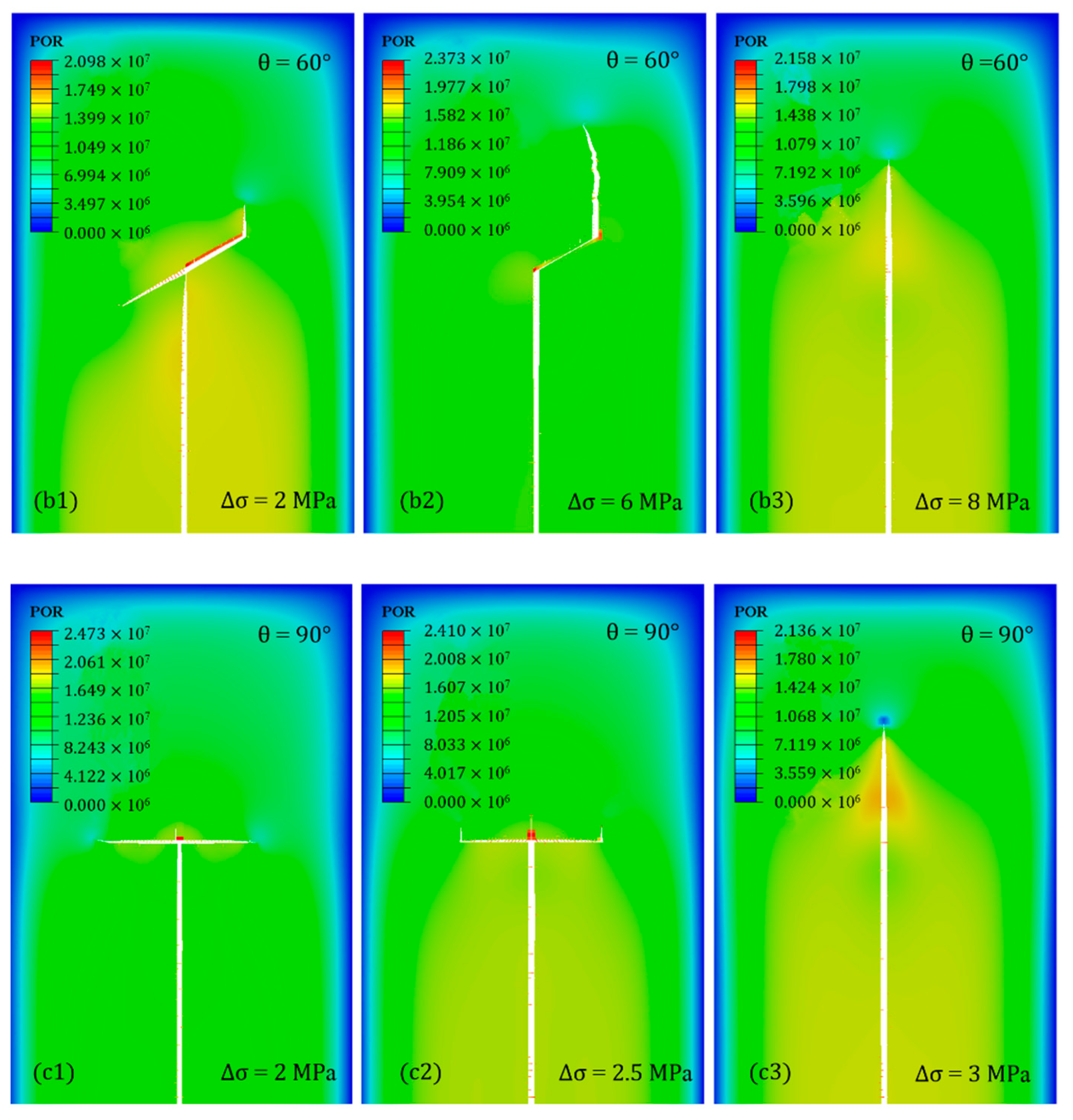Even though the scales of the parameter values in the numerical models were different from those of the laboratory fracturing experiments, considering the model dimensions, the numerical simulation results demonstrated in Figure 6 show strong agreement with the experimental results detailed in the literature. The results reveal that the approaching angle of a natural fracture and the stress difference have a strong effect on the morphology of fracture propagation. As shown in Figure 6, when $\nabla \sigma$ < 2 MPa and Q = 0.0005 m³/s, all the HFs propagate along the NF with two fracture directions. However, as $\nabla \sigma$ increases, the HF can open the NF, but only in the direction of the large intersection angle. When the stress difference is large enough, all the HFs will cross the NF to form a long planar fracture, which demonstrates that stress difference is the key factor when HFs intersect with the NF. The HFs tend to cross the NF at any approaching angle when the stress difference is high. Furthermore, a HF is more likely to open and propagate along the NF when the stress difference is low. The smaller the approaching angle of the NF, the higher the critical difference stress for HF crossing will be. The lower the approaching angle of the NF, the easier it is to open two sides of the NF. The numerical simulation results are consistent with experimental results that have been published [25,28,29], as shown in Figure 7. For better visualization, we connected the critical opening pressure at different approaching angles, which is presented as a red line and acts as a comparison standard of our numerical model. It can be seen that HF is more likely to cross the NF above the red critical line; however, the HF is inclined to open the NF below the critical line.

3.2. Horizontal Stress Difference

Figure 6 shows that an increase in horizontal stress difference tends to increase the probability of NFs crossing under lower values of the approaching angle. However, the stress shadow resulting from multi-fractures can change this phenomenon in multiple-cluster hydraulic fracturing. Figure 8 shows HF geometries under different stress anisotropies ∇σ in a pre-existing NF system. We assigned the variables as θ = 60°, Q = 0.0005 m³/s, and µ = 1 mPa·s. All models in this section adopted a two-clusters configuration with a spacing of 40 m. The results show that HFs tend to cross the NFs and form a less complex fracture network as the horizontal stress difference increases, which agrees well with the findings of Zou et al. [7]. In the isotropic case of ∇σ = 2 MPa, the HFs that initiate from the two perforation clusters mainly open and propagate along the NFs, resulting in a highly complex fracture network near the horizontal wellbore. However, the geometry of HFs change with the propagation process owing to stress interference. As shown in Figure 8a, two HFs propagate in opposite directions, deviating from each other, which leads to more opportunities for the right HFs to open NFs and for the left HFs to cross the NFs. When the stress difference increases, the complexity of the fracture network reduces, and fractures propagate in a more straight manner within the same injection process [11]. In addition, during a propagation process, HF growth can be suppressed because of back stress induced by other propagating HFs (Figure 8b,c). Under a horizontal stress difference of 8 MPa (Figure 8d), almost all NFs are crossed by HFs instead of deflecting, which causes less complex fracture networks.

With stronger stress anisotropy, HFs tend to pass through NFs and form smaller curvatures in the propagation path [30], which results in narrower, longer, and less complex fracture networks. Furthermore, the influence of back stress will be more significant, which aggravates the diversion behavior of HFs and changes the crossing phenomenon between HFs and NFs. Therefore, it is beneficial to form more complex fracture networks at lower fracture differences (∇σ < 8 MPa). As shown in Figure 9, the total fracture network length decreases as the stress difference increases. The total fracture length reduced by 38.26 m when stress difference increased from 2 to 8 MPa, but only reduced by 0.8 m as the stress difference increased from 6 to 8 MPa. This demonstrates that fluid driven fractures can propagate widely and are connected to more natural fractures at lower stress differences, which is useful for connecting the flow channel.

3.3. Spacing of Perforation Clusters

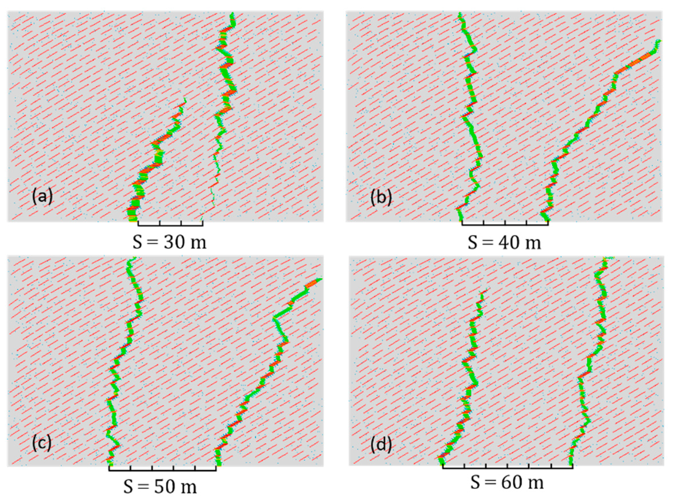
When the cluster spacing is small, the mechanical interaction between adjacent fractures is obvious, and a less complex fracture network can be formed [30]. Figure 10 shows the propagation path of multiple fractures in a natural fracture system with a cluster spacing of 30, 40, 50 and 60 m. The parameters Q = 0.0005 m³/s, µ = 1 mPa·s, $\nabla \sigma$ = 3 MPa were set for the simulation. It can be seen that different cluster spacing has a significant effect on fracture morphology. As the cluster spacing increases, the influence of the stress shadow among adjacent fractures is alleviated, which results in more opening phenomena among HFs and NFs. Given S = 30 m in Figure 10a, the multiple HFs initiate from the wellbore and then intersect with the NFs. With the fracturing process, the stress shadow becomes more severe and obvious suppression can be observed in one of the NFs. Further, the suppressed fractures propagate, becoming wider and shorter. However, unsuppressed fractures extended rapidly, resulting in a longer and narrower fracture network. When the cluster spacing increases (Figure 10b–d), the HFs propagate quickly from the wellbore and experience less suppression compared with the case of S = 30 m. The interference of each cluster decreases as cluster spacing increases. Meanwhile, the orientation of the crack tip is also alleviated under this condition, especially when S is larger than 60 m. For the purpose of maximizing the fracture network, deeper propagation should be provided to connect more NFs. Therefore, production can be improved by increasing the perforation cluster spacing within a relative range.

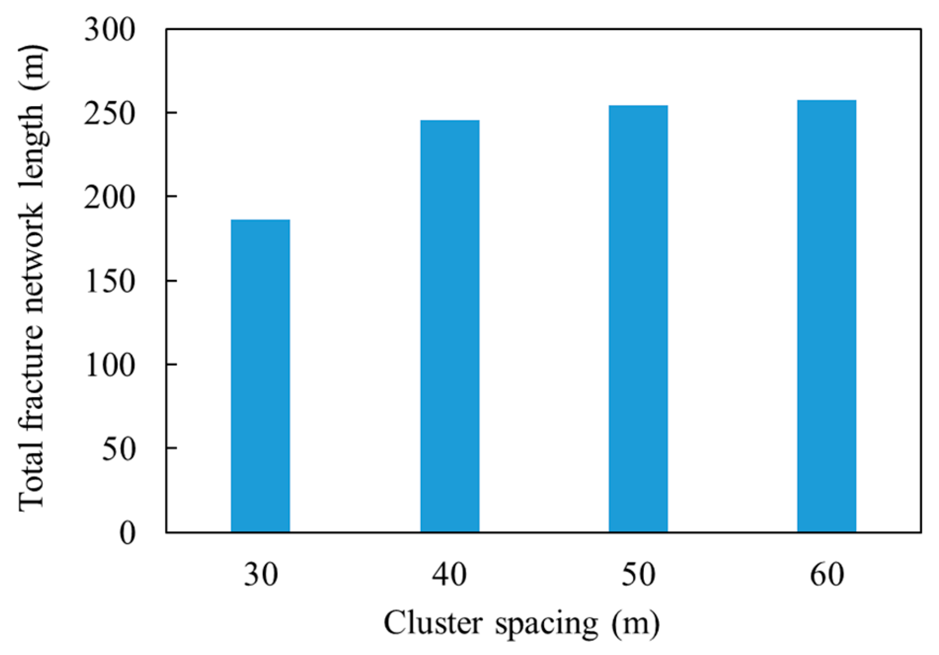
Reducing the cluster spacing is beneficial to improving the complexity of the fracture network under the low stress difference condition [31]. However, numerical simulation in this work gave contrary results: Propagation suppression of multiple fractures occurred with a low stress difference, which caused shorter fracture propagation. Moreover, owing to serious stress interference at lower cluster spacing, a greater amount of crossing can be observed between HFs and NFs, which can reduce the simulated reservoir volume [32]. As shown in Figure 11, the total fracture network length increases when the cluster spacing changes from 30 to 40 m; however, when the spacing is greater than 40 m, the total length does not change significantly. As a result, short perforation cluster spacing should be avoided to increase the complexity of the fracture network. In this case, the optimization of the cluster spacing is recommended to vary from 40 to 60 m, which is suggested by considering not only the influence of stress shadowing but also the controlling area for improving production.

3.4. Injection Rate of Fracturing Fluid

The influence of the fracturing fluid on the geometric shape of HFs can be expressed by the injection rate and fluid viscosity. In this section, the influence of the injection rate is discussed. It is concluded that by increasing the injection rate, the fluid injection pressure increases [4]. Owing to a high propagation pressure, HFs have more chance to pass through NFs and tend to form lager planar hydraulic fractures [33]. A pre-existing fracture system with random lengths and an approaching angle of 60° was introduced to investigate the influence of injection rate on the fracture network. The stress difference, fluid viscosity and cluster spacing remained constant at 3 MPa, 1 mPa·s, and 40 m, respectively. As shown in Figure 12, three types of flow rates were used: Q = 0.0001 m³/s, Q = 0.0005 m³/s and Q = 0.001 m³/s. It can be seen that the fracturing of two clusters initiated at the wellbore and reactive NFs at an earlier stage of injection. With the fracturing procedure, the fractures divert in opposite directions at lower injection rates, as shown in Figure 12a,b. However, the morphologies of the two-cluster HFs change less when the fluid rate increases from 0.0001 to 0.0005 m³/s. When the injection rate reaches 0.001 m³/s, it has a significant influence on the complexity of the fracture network. As shown in Figure 12c, HFs propagate in a straighter manner perpendicular to the horizontal minimum principle stress, which results in more crossing phenomena and a less complex fracture network.

A high injection rate during the entire process may reduce the complexity of the fracture network due to the high net pressure that will be formed; as a result, the probability of fracture crossing would increase. The total length of the fracture network reduced considerably when the injection rate increased from 0.0005 to 0.001 m³/s, which resulted in a reduction of flow channel and make the release of gas and oil difficult, as shown in Figure 13. However, a high injection rate can create larger far-field propagation of the fracture network [34], which is mainly due to reduced connection in the near wellbore and deeper propagation of the fracture network. Therefore, various injection rates should be adopted to maximize the complexity of the fracture network. The large fluid pressure within a fracture due to high injection rates can be used to form straighter fracture networks, and deeper propagation at the early stage of fracturing. A low injection rate can open more NFs and creates more diversions in the wider control area in the later period of fracturing. By controlling the injection rates, a large filed of fracture network can be realized.

3.5. Viscosity of the Pumping Fluid

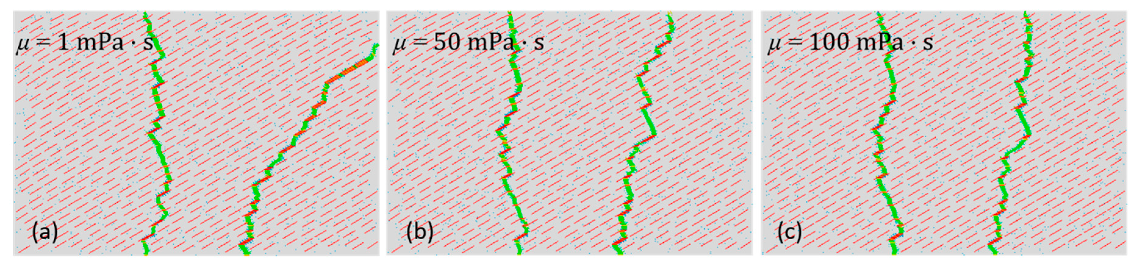
During the fracturing of naturally fractured reservoirs, it was found that the morphology and complexity of the fracture are closely related to the fracture net pressure, which is mainly determined by the fracturing fluid viscosity and injection rate. In this section, three types of numerical models with different viscosities were simulated to investigate the influence of the fracturing viscosity. The results in Figure 14 reveal that fracturing viscosity can affect the morphology and complexity of fractures, especially if it has a high value. In this simulation the stress difference, flow rate, and cluster spacing remained constant at 3 MPa, 0.0005 m³/s and 40 m, respectively. Figure 14a shows that HFs tend to open more NFs and propagate along the NFs at a low viscosity condition of µ = 1 mPa·s. Meanwhile, the preference for diverting to the opposite direction for each cluster fracture is enhanced with low viscosity fracturing fluid. However, Beguelsdijk et al. [35] found that a fracturing fluid with a high viscosity could induce separate propagation on an optimal fracture surface. For this reason, more opening of NFs may increase the complexity of the fracture network, which will increase the possibility of separate propagation. In addition, more straight fractures will be formed along the direction of maximum horizontal stress, which will result in the formation of a simple fracture network, as shown in Figure 14b,c. The morphology and complexity of fractures will change obviously when the viscosity increases from 1 to 50 mPa·s; however, few transformations can be obtained when the viscosity varies from 50 to 100 mPa·s. Hence, it can be concluded that lower range viscosities have a greater effect on fracture morphology than higher range viscosities.

For the purpose of maximizing the stimulated reservoir volume (SRV), deeper propagation in the far-field region and less tortuosity near the wellbore should be generated for a complex fracture network. A high viscosity during the early stage of fracturing can promote deeper propagation of HFs and reduce the tortuosity near the wellbore. Later, a lower viscosity can activate more NFs and enhance the propagation with the approaching angle, thus forming a more complex fracture network. Figure 15 shows that a lower injection viscosity can lead to the formation of a large fracture network: when the viscosity is 1 mPa·s, the total fracture network length is 254.4 m. Therefore, higher production of oil and gas can be achieved by a lower injection fracturing treatment. More simulations should be conducted to further investigate whether viscosity induce can separate propagation with a random pre-existing NF system.

3.6. Number of Perforation Clusters

Different hydraulic fracturing can result in different HF morphologies because of stress interference. For multiple-cluster hydraulic fracturing, the number of perforation clusters has a significant influence on fracture propagation; this can be seen from the six pictures in Figure 16. A fracture’s geometric shape is significantly affected by the numbers of clusters at different fracturing times. When the stress difference, fluid rate, cluster spacing and viscosity are fixed at Q = 0.0005 m³/s, µ = 1 mPa·s, S = 40 m and $\nabla \sigma$ = 3 MPa, the fracture propagation morphologies are comparable in these cases. In this section, three types of perforation configurations (two, three and four clusters) were modeled to investigate the effect of perforation application. The results reveal that the interference of the stress shadow plays a major role in fracture propagation, as it may make the propagation undesirable for production. The resulting mechanical action alters the value and direction of in situ stress, which results in unexpected suppression of the fracture’s propagation. As shown in the two-clusters perforation configuration (Figure 16(a1,a2)), back stress causes the left fracture to be suppressed, exhibiting shorter and wider networks compared with the right fracture. The middle fracture seems to be significantly influenced, forming shorter and wider HFs in Figure 16(b1,b2), compared with the fractures at either side. For the four-cluster configuration (Figure 16(c1,c2)), one fracture can break though and propagate into the deep reservoirs rapidly, while the residuary fractures tend to be suppressed more or less. Further, it can be observed from Figure 16 that the fracturing time will affect the morphology of the HFs to differing degrees. All of the configurations show that there is less influence on the morphology of HFs in the early stage of fracturing (i.e., T = 500 s), which is probably due to less spreading of net pressure in the fracture network.

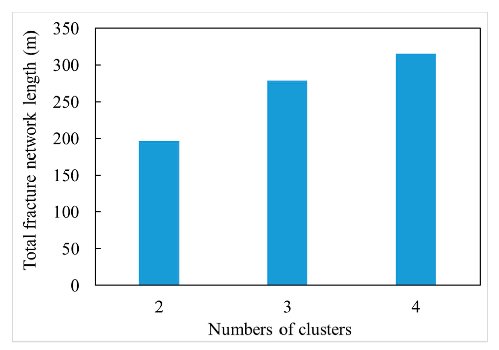
An increase in the perforation number will increase the interaction between HFs and NFs, and the propagation path will be easier to be maintain. Meanwhile, the interference area of the stress shadow will increase with an increase in fracturing time, and the propagation path will be easily altered. As shown in Figure 17, the volume of the fracture network increases rapidly as the number of clusters increases. For instance, the total fracture length increases to 315 m when the number of clusters is set to four. Although larger numbers of cluster can increase the volume of the fracture network, strong interference from multiple clusters can result in considerable suppression of the lateral clusters. In that situation, a shorter and wider facture network will be generated, which goes against fluid release from the formation to the fracture channel. Therefore, lower cluster spacing with multiple clusters should be avoided, as it will increase the serious interference due to stress shadow, which results in a suppressed fracture network.

4. Conclusions

Using a 2D FEM model based on the PPCZ method, we performed a series of simulation models coupling seepage and stress to investigate the mechanism of fracture network propagation in naturally fractured reservoirs. At the same time, a python code written by the authors was used to incorporate pore pressure elements for modeling the fractures and the joints of the crossed fractures. Several geological and engineering factors influencing the fracture propagation pattern were applied to conduct sensitive analyses. The main propagation rules can be concluded as:

(1)

The horizontal differential stress dominates main propagation patterns of the hydraulic fracture network. The morphology of a hydraulic fracture may change from being randomly diverted to more straight as the horizontal differential stress increases. The fluid driven fracture nearly crosses NFs to extend simple transverse fractures when the differential stress exceeds 8 MPa at an approaching angle of 60°, according to our FEM models.

(2)

The viscosity and injection rate of the fracturing fluid affect the development of the fracture network at different fracturing times. The fracture network area can reach its maximum with various injection rates and viscosities during different fracturing stages. Using a higher injection rate and fluid viscosity appears to raise the net pressure, which will increase the capacity of a HF to cross the NFs near the wellbore and facilitate a deeper propagation into the formations.

(3)

Using a short cluster spacing at 30 m will result in unexpected consequences where one or more fractures will be suppressed to form short and simple transverse fractures. Nevertheless, the phenomenon of suppression could weaken when the cluster spacing distance increases from 40 to 60 m.

(4)

Cluster spacing should be taken into consideration as the increase of cluster numbers causes enhanced stress interference. Due to tremendous suppression and merging of fractures under multiple stress interference, increasing the cluster number is meaningless with lower cluster spacing.

References

1. Zhang, X.; Jeffrey, R.G. Role of overpressurized fluid and fluid-driven fractures in forming fracture networks. J. Geochem. Explor. 2014, 144, 194–207. [Google Scholar] [CrossRef]
2. Zhang, X.; Jeffrey, R.G.; Wu, B. Mechanics of edge crack growth under transient pressure and temperature conditions. Int. J. Solids Struct. 2015, 69–70, 11–22. [Google Scholar] [CrossRef]
3. Olson, J.E. Multi-fracture propagation modeling: Applications to hydraulic fracturing in shales and tight gas sands. In Proceedings of the 42nd U.S. Rock Mechanics Symposium: ARMA, San Francisco, CA, USA, 29 June–2 July 2008. [Google Scholar]
4. Hamidi, F.; Mortazavi, A. A new three dimensional approach to numerically model hydraulic fracturing process. J. Pet. Sci. Eng. 2014, 124, 451–467. [Google Scholar] [CrossRef]
5. Yan, C.; Zheng, H. A two-dimensional coupled hydro-mechanical finite-discrete model considering porous media flow for simulating hydraulic fracturing. Int. J. Rock Mech. Min. Sci. 2016, 88, 115–128. [Google Scholar] [CrossRef]
6. Zuo, Y.; Ma, X.; Zhang, S.; Zhou, T.; Li, H. Numerical Investigation into the Influence of Bedding Plane on Hydraulic Fracture Network Propagation in Shale Formations. Rock Mech. Rock Eng. 2016, 49, 3597–3614. [Google Scholar] [CrossRef]
7. Zou, Y.; Zhang, S.; Ma, X.; Zhou, T.; Zeng, B. Numerical investigation of hydraulic fracture network propagation in naturally fractured shale formations. J. Struct. Geol. 2016, 84, 1–13. [Google Scholar] [CrossRef]
8. Fatahi, H.; Hossain, M.M.; Sarmadivaleh, M. Numerical and experimental investigation of the interaction of natural and propagated hydraulic fracture. J. Nat. Gas Sci. Eng. 2017, 37, 409–424. [Google Scholar] [CrossRef]
9. Olson, J.E.; Taleghani, A.D. Modeling simultaneous growth of multiple hydraulic fractures and their interaction with natural fractures. In Proceedings of the SPE Hydraulic Fracturing Technology Conference, The Woodlands, TX, USA, 19–21 January 2009. [Google Scholar]
10. Kan, W.; Olson, J.E. Numerical investigation of complex hydraulic fracture development in naturally fractured reservoirs. Int. J. Health Geogr. 2015, 6, 1–15. [Google Scholar]
11. Zhang, S.-C.; Lei, X.; Zhou, Y.-S.; Xu, G.-Q. Numerical simulation of hydraulic fracture propagation in tight oil reservoirs by volumetric fracturing. Pet. Sci. 2015, 12, 674–682. [Google Scholar] [CrossRef] [Green Version]
12. Li, Y.; Deng, J.G.; Liu, W.; Feng, Y. Modeling hydraulic fracture propagation using cohesive zone model equipped with frictional contact capability. Comput. Geotech. 2017, 91, 58–70. [Google Scholar] [CrossRef]
13. Sarris, E.; Papanastasiou, P. The influence of the cohesive process zone in hydraulic fracturing modelling. Int. J. Fract. 2011, 167, 33–45. [Google Scholar] [CrossRef]
14. Carrier, B.; Granet, S. Numerical modeling of hydraulic fracture problem in permeable medium using cohesive zone model. Eng. Fract. Mech. 2012, 79, 312–328. [Google Scholar] [CrossRef] [Green Version]
15. Chen, Z. Finite element modelling of viscosity-dominated hydraulic fractures. J. Pet. Sci. Eng. 2012, 88–89, 136–144. [Google Scholar] [CrossRef]
16. Shen, X.; Cullick, S. Numerical Modeling of Fracture Complexity with Application to Production Stimulation; Elsevier: Amsterdam, The Netherlands, 2012; p. A6. [Google Scholar]
17. Haddad, M.; Sepehrnoori, K. Cohesive Fracture Analysis to Model Multiple-Stage Fracturing in Quasibrittle Shale Formations. In Proceedings of the Simulia Community Conference, Providence, RI, USA, 19–22 May 2014. [Google Scholar]
18. Guo, J.; Zhao, X.; Zhu, H.; Zhang, X.; Pan, R. Numerical simulation of interaction of hydraulic fracture and natural fracture based on the cohesive zone finite element method. J. Nat. Gas Sci. Eng. 2015, 25, 180–188. [Google Scholar] [CrossRef]
19. Guo, J.; Luo, B.; Lu, C.; Lai, J.; Ren, J. Numerical investigation of hydraulic fracture propagation in a layered reservoir using the cohesive zone method. Eng. Fract. Mech. 2017, 186, 195–207. [Google Scholar] [CrossRef]
20. Yao, Y. Linear Elastic and Cohesive Fracture Analysis to Model Hydraulic Fracture in Brittle and Ductile Rocks. Rock Mech. Rock Eng. 2012, 45, 375–387. [Google Scholar] [CrossRef]
21. Shin, D.H.; Sharma, M.M. Factors Controlling the Simultaneous Propagation of Multiple Competing Fractures in a Horizontal Well; Pearson/Prentice Hall: Upper Saddle River, NJ, USA, 2014; pp. 816–819. [Google Scholar]
22. Batchelor, G.K. An Introduction to Fluid Dynamics; Cambridge University Press: Cambridge, UK, 1967; pp. 1–29. [Google Scholar]
23. Biot, M.A. General Theory of Three-Dimensional Consolidation. J. Appl. Phys. 1941, 12, 155–164. [Google Scholar] [CrossRef]
24. Guo, T.; Zhang, S.; Qu, Z.; Zhou, T.; Xiao, Y.; Gao, J. Experimental study of hydraulic fracturing for shale by stimulated reservoir volume. Fuel 2014, 128, 373–380. [Google Scholar] [CrossRef]
25. Blanton, T.L. Propagation of Hydraulically and Dynamically Induced Fractures in Naturally Fractured Reservoirs. In Proceedings of the SPE Unconventional Gas Technology Symposium, Louisville, KY, USA, 18–21 May 1986. [Google Scholar]
26. Zhou, J.; Jin, Y.; Chen, M. Experimental investigation of hydraulic fracturing in random naturally fractured blocks. Int. J. Rock Mech. Min. Sci. 2010, 47, 1193–1199. [Google Scholar] [CrossRef]
27. Yushi, Z.; Shicheng, Z.; Tong, Z.; Xiang, Z.; Tiankui, G. Experimental Investigation into Hydraulic Fracture Network Propagation in Gas Shales Using CT Scanning Technology. Rock Mech. Rock Eng. 2015, 49, 33–45. [Google Scholar] [CrossRef]
28. Warpinski, N.R.; Teufel, L.W. Influence of geologic discontinuities on hydraulic fracture propagation. J. Pet. Technol. 1984, 39, 209–220. [Google Scholar] [CrossRef]
29. Gu, H.; Weng, X.; Lund, J.B.; Mack, M.G.; Ganguly, U.; Suarez-Rivera, R. Hydraulic Fracture Crossing Natural Fracture at NonOrthogonal Angles, A Criterion, Its Validation and Applications. In SPE Production & Operations; Society of Petroleum Engineers: Houston, TX, USA, 2011. [Google Scholar]
30. Zeng, Q.; Yao, J. Numerical simulation of fracture network generation in naturally fractured reservoirs. J. Nat. Gas Sci. Eng. 2016, 30, 430–443. [Google Scholar] [CrossRef]
31. Manchanda, R.; Roussel, N.P.; Sharma, M.M. Factors influencing fracture trajectories and fracturing pressure data in a horizontal completion. In Proceedings of the 46th U.S. Rock Mechanics/Geomechanics Symposium, Chicago, IL, USA, 24–27 June 2012. [Google Scholar]
32. Bunger, A.P.; Jeffrey, R.G.; Kear, J.; Zhang, X.; Morgan, M. Experimental investigation of the interaction among closely spaced hydraulic fractures. In Proceedings of the 45th U.S. Rock Mechanics/Geomechanics Symposium, San Francisco, CA, USA, 26–29 June 2011. [Google Scholar]
33. Guo, T.; Zhang, S.; Zou, Y.; Xiao, B. Numerical simulation of hydraulic fracture propagation in shale gas reservoir. J. Nat. Gas Sci. Eng. 2015, 26, 847–856. [Google Scholar] [CrossRef]
34. Liu, C.; Shi, F.; Zhang, Y.; Zhang, Y.; Deng, D.; Wang, X.; Liu, H.; Wu, H. High injection rate stimulation for improving the fracture complexity in tight-oil sandstone reservoirs. J. Nat. Gas Sci. Eng. 2017, 42, 133–141. [Google Scholar] [CrossRef]
35. Beugelsdijk, L.J.L.; de Pater, C.J.; Sato, K. Experimental hydraulic fracture propagation in a multi-fractured medium. In Proceedings of the SPE Asia Pacific Conference on Integrated Modelling for Asset Management, Yokohama, Japan, 25–26 April 2000. [Google Scholar]
Figure 1. Fracturing flow pattern within the cohesive element.
Processes 07 00028 g001
Figure 2. Normal fracturing flow for permeable cohesive surfaces.
Processes 07 00028 g002
Figure 3. Quadratic nominal stress traction and separation law.
Processes 07 00028 g003
Figure 4. Cohesive linear-softening for the Benzeggagh–Kenane (BK) criterion.
Processes 07 00028 g004
Figure 5. Multiple-cluster model with a 60° approach angle for natural fractures (NFs).
Processes 07 00028 g005
Figure 6. Effect of approaching angle and stress difference on hydraulic fracture propagation. (a1a3) Approaching angle = 45°: stress difference = 2, 8, and 12 MPa, respectively; (b1b3) approaching angle = 60°: stress difference = 2, 6, and 8 MPa, respectively; (c1c3) approaching angle = 90°: stress difference = 2, 2.5, and 3 MPa, respectively.
Processes 07 00028 g006aProcesses 07 00028 g006b
Figure 7. Comparison between numerical simulation and experimental results with different angles of approach and horizontal differential stresses.
Processes 07 00028 g007
Figure 8. Effect of stress difference on hydraulic fracture propagation. (a) Stress difference = 2 MPa; (b) stress difference = 4 MPa; (c) stress difference = 6 MPa; (d) stress difference = 8 MPa.
Processes 07 00028 g008
Figure 9. Fracture network lengths at different horizontal stress differences.
Processes 07 00028 g009
Figure 10. Effect of cluster spacing on hydraulic fracture propagation. (a) Cluster spacing = 30 m; (b) cluster spacing = 40 m; (c) cluster spacing = 50 m; (d) cluster spacing = 60 m.
Processes 07 00028 g010
Figure 11. Fracture network lengths at different cluster spacing distances.
Processes 07 00028 g011
Figure 12. Effect of fluid rate on hydraulic fracture propagation. (a) Injection rate = 0.0001 m3/s; (b) injection rate = 0.0005 m3/s; (c) injection rate = 0.001 m3/s.
Processes 07 00028 g012
Figure 13. Fracture network lengths at different injection rates.
Processes 07 00028 g013
Figure 14. Effect of viscosity on hydraulic fracture propagation. (a) Fluid viscosity = 1 mPa∙s; (b) fluid viscosity = 50 mPa∙s; (c) fluid viscosity = 100 mPa∙s.
Processes 07 00028 g014
Figure 15. Fracture network lengths achieved with different injection fluid viscosities.
Processes 07 00028 g015
Figure 16. Effect of cluster numbers on hydraulic fracture propagation. (a1,a2) Two clusters fracturing scenario at fracturing time T = 500, 1200 s; (b1,b2) three clusters fracturing scenario at fracturing time T = 500, 1200 s; (c1,c2) four clusters fracturing scenario at fracturing time T = 500, 1200 s.
Processes 07 00028 g016
Figure 17. Fracture network lengths corresponding to different numbers of clusters.
Processes 07 00028 g017