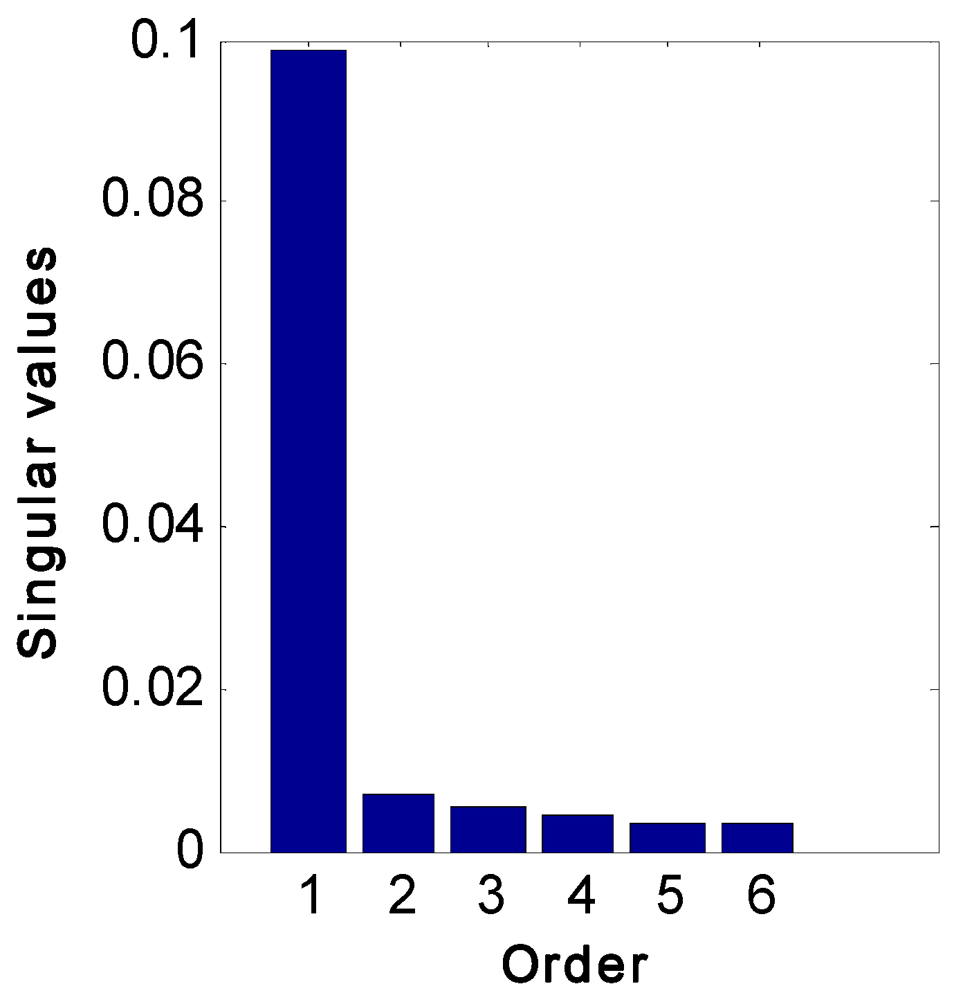
Figure 1.
Singular values of the matrix , Equation (3), resulting from input/output data collected for a distillation column excited by pseudo random binary sequence (PRBS) inputs.
Figure 1.
Singular values of the matrix , Equation (3), resulting from input/output data collected for a distillation column excited by pseudo random binary sequence (PRBS) inputs.
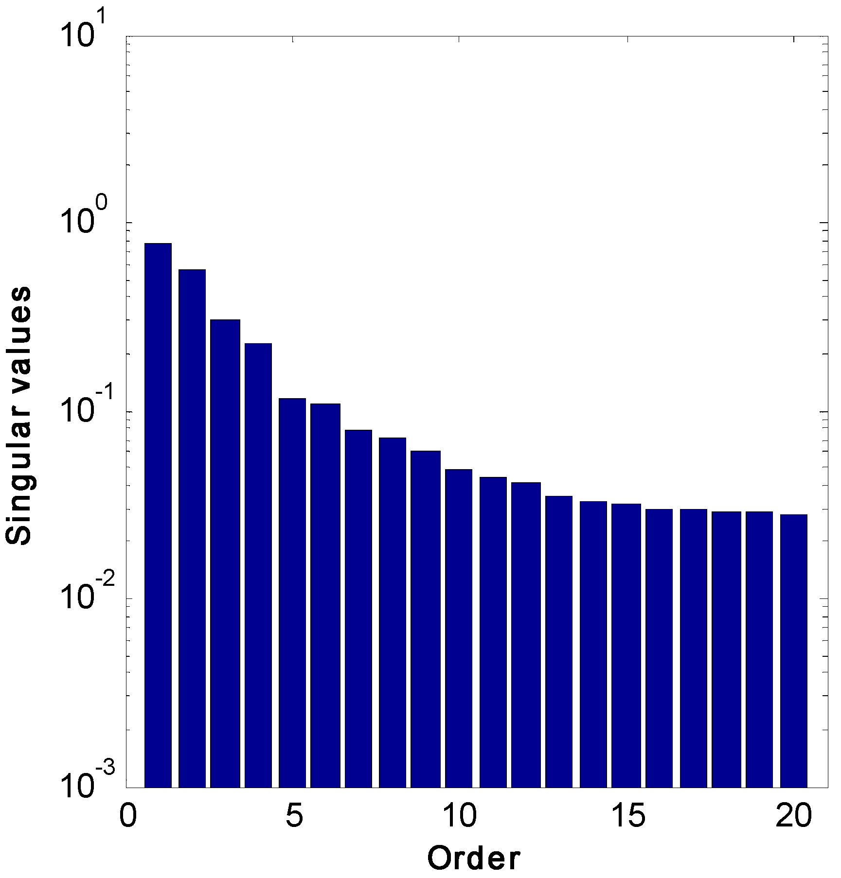
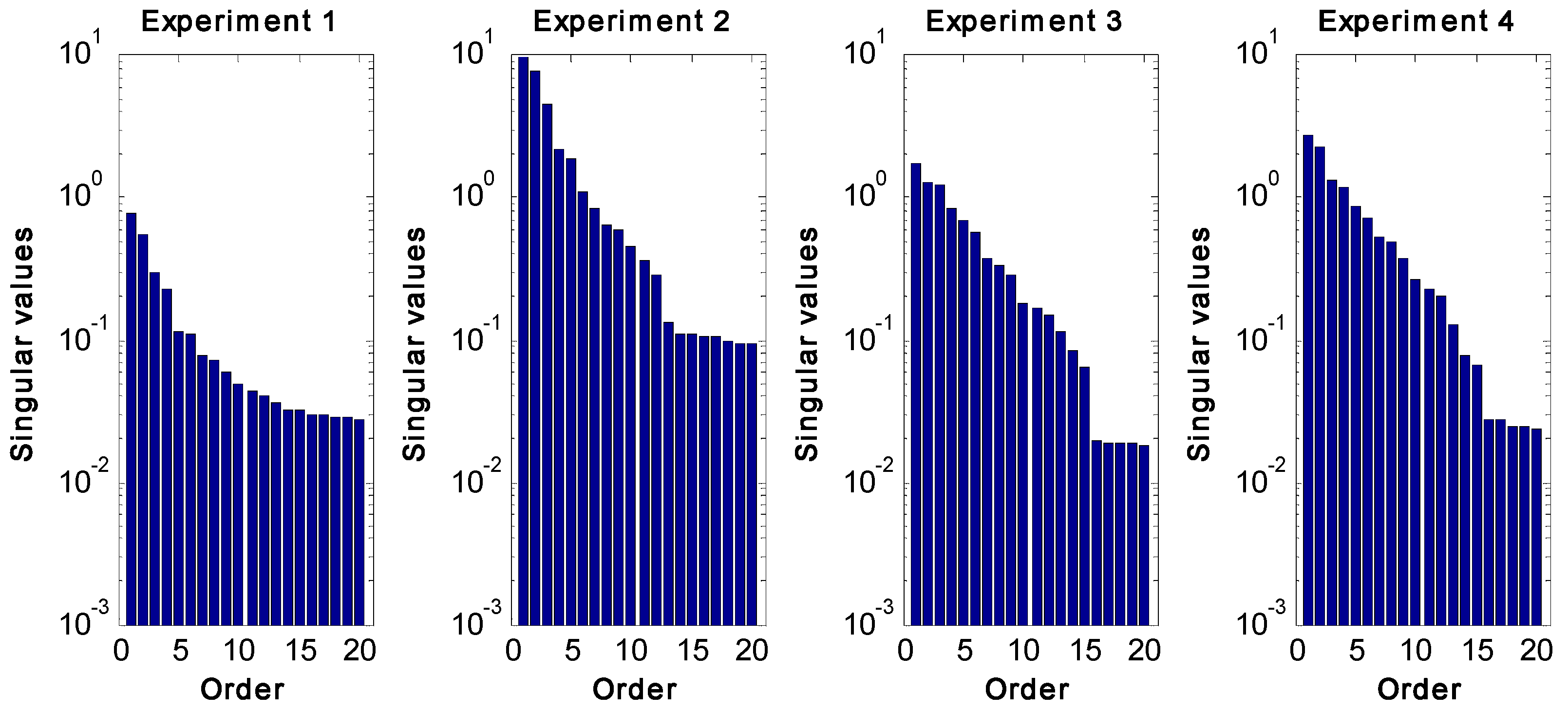
Figure 2.
Singular values of the matrix , Equation (3), resulting from input/output data collected for a fluidized catalytic cracking (FCC) system excited by PRBS inputs.
Figure 2.
Singular values of the matrix , Equation (3), resulting from input/output data collected for a fluidized catalytic cracking (FCC) system excited by PRBS inputs.
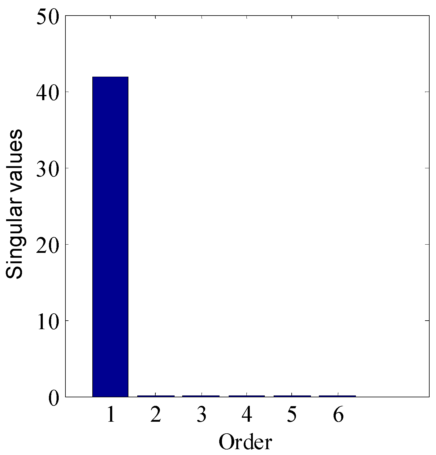
Figure 3.
Model order estimation for distillation column using experimental data from a process excited by rotated PRBS inputs at the wrong rotation angle of in place of the correct rotation angle of .
Figure 3.
Model order estimation for distillation column using experimental data from a process excited by rotated PRBS inputs at the wrong rotation angle of in place of the correct rotation angle of .
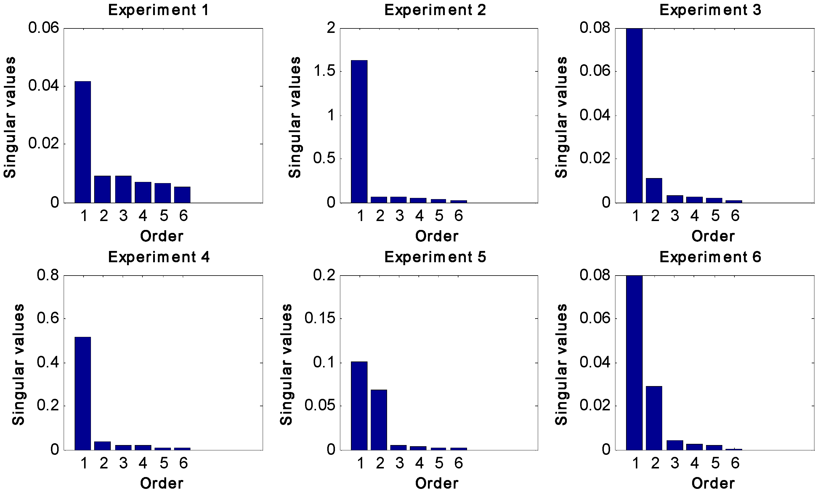
Figure 4.
Order estimation for distillation column using adaptive DOE with rotated PRBS inputs. A cut-off point is evident at two.
Figure 4.
Order estimation for distillation column using adaptive DOE with rotated PRBS inputs. A cut-off point is evident at two.
Figure 5.
Order estimation for a FCC system using adaptive DOE with rotated PRBS inputs. A cut-off point is evident at 15.
Figure 5.
Order estimation for a FCC system using adaptive DOE with rotated PRBS inputs. A cut-off point is evident at 15.
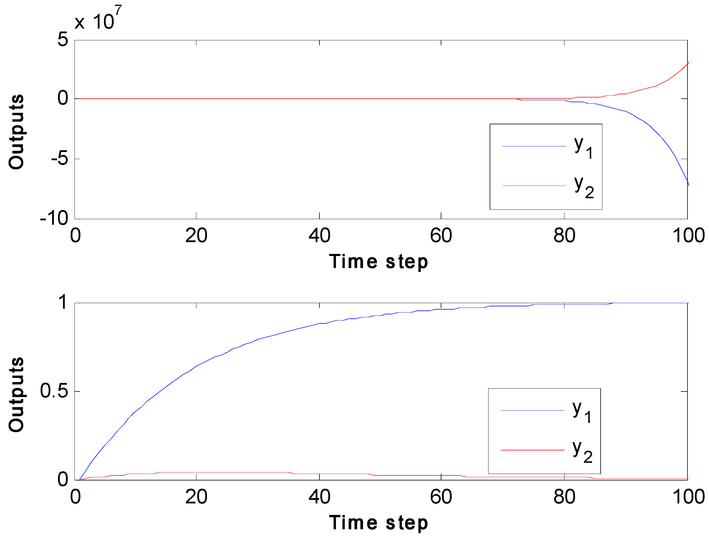
Figure 6.
Closed-loop output response for step change in the set point of Output-1 () and no change in the set point of Output-2 () using controllers based on model (top) and (bottom), respectively.
Figure 6.
Closed-loop output response for step change in the set point of Output-1 () and no change in the set point of Output-2 () using controllers based on model (top) and (bottom), respectively.
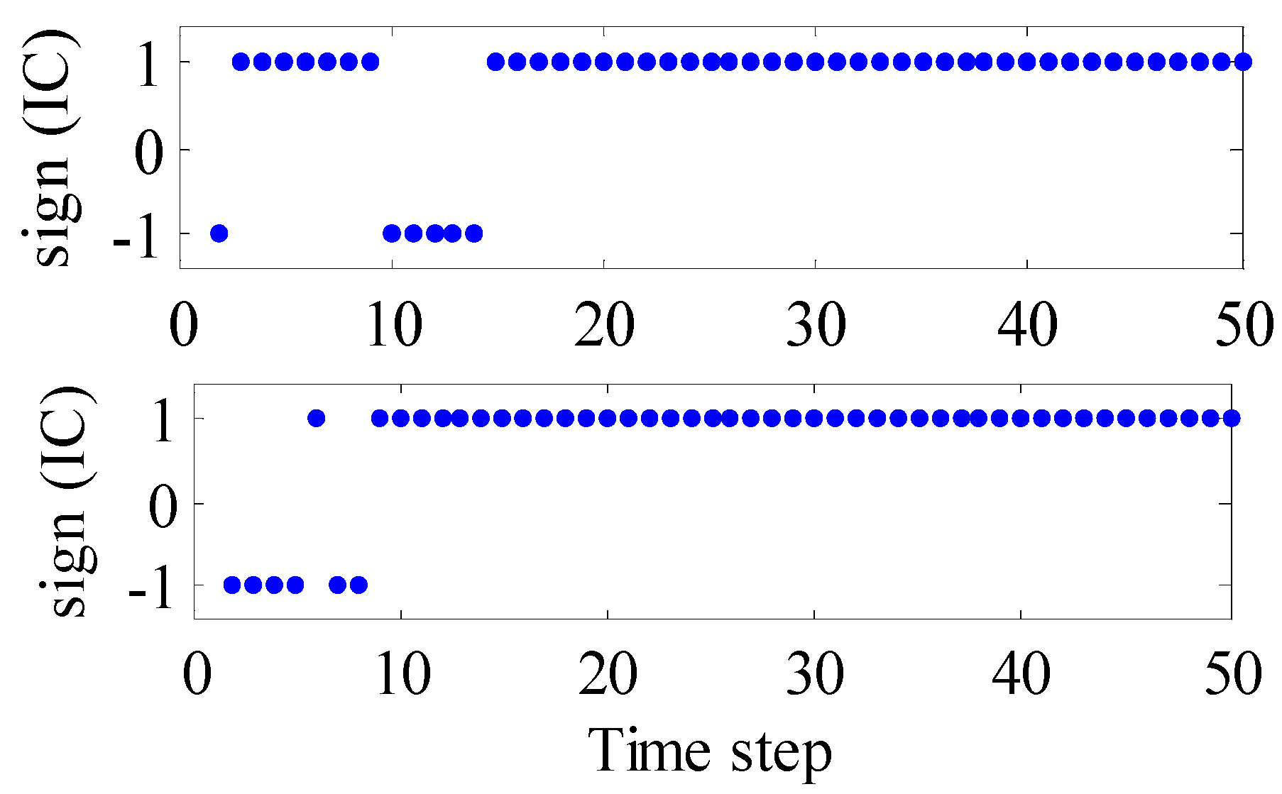
Figure 7.
Satisfaction (+1) or violation (−1) of IC for the identified model when (top row) and (bottom row). Integral controllability (IC) checked via Equation (11) for both cases.
Figure 7.
Satisfaction (+1) or violation (−1) of IC for the identified model when (top row) and (bottom row). Integral controllability (IC) checked via Equation (11) for both cases.
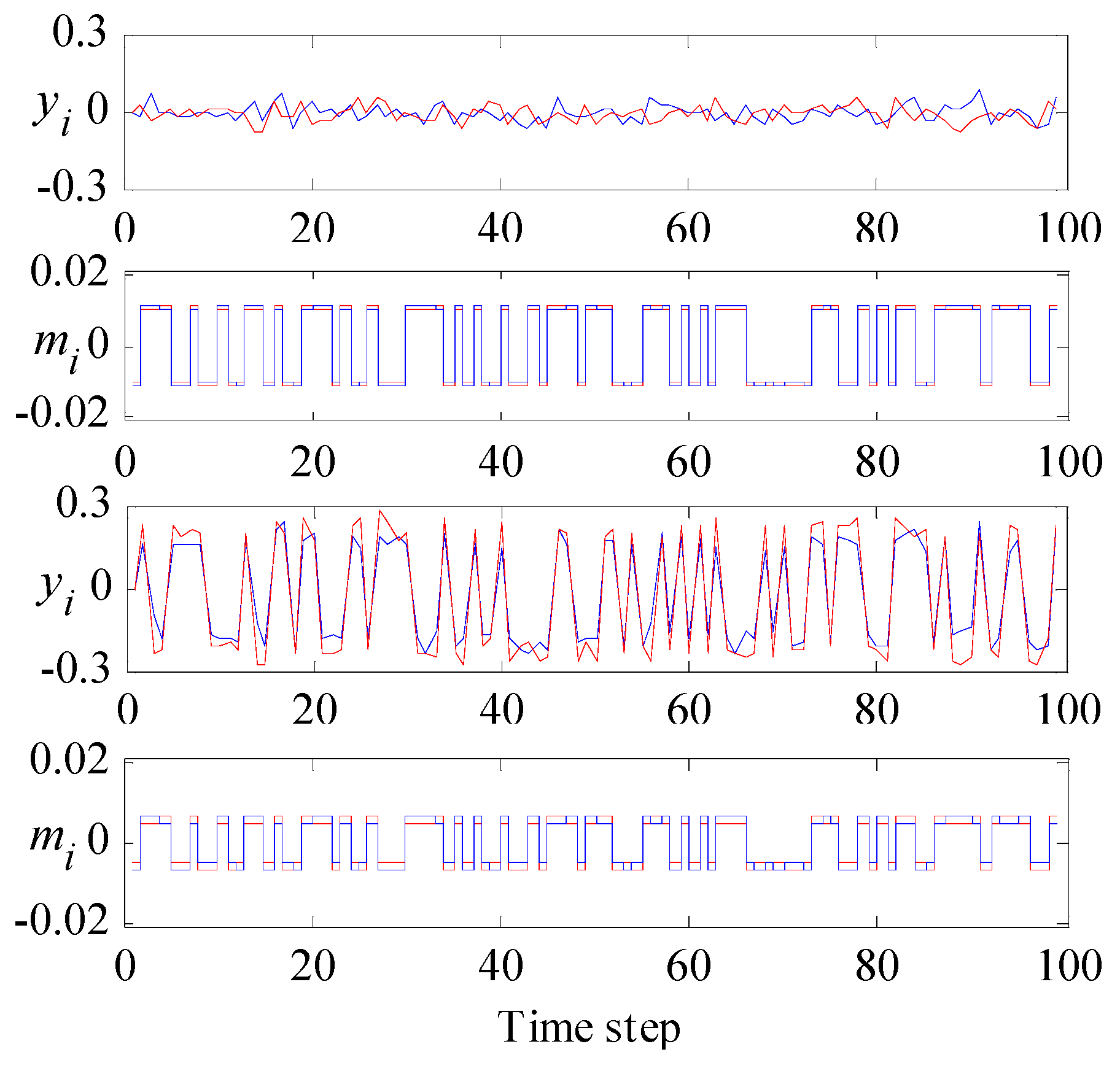
Figure 8.
Outputs, , and inputs, (), for IC optimal design when (top two rows) and (bottom two rows).
Figure 8.
Outputs, , and inputs, (), for IC optimal design when (top two rows) and (bottom two rows).
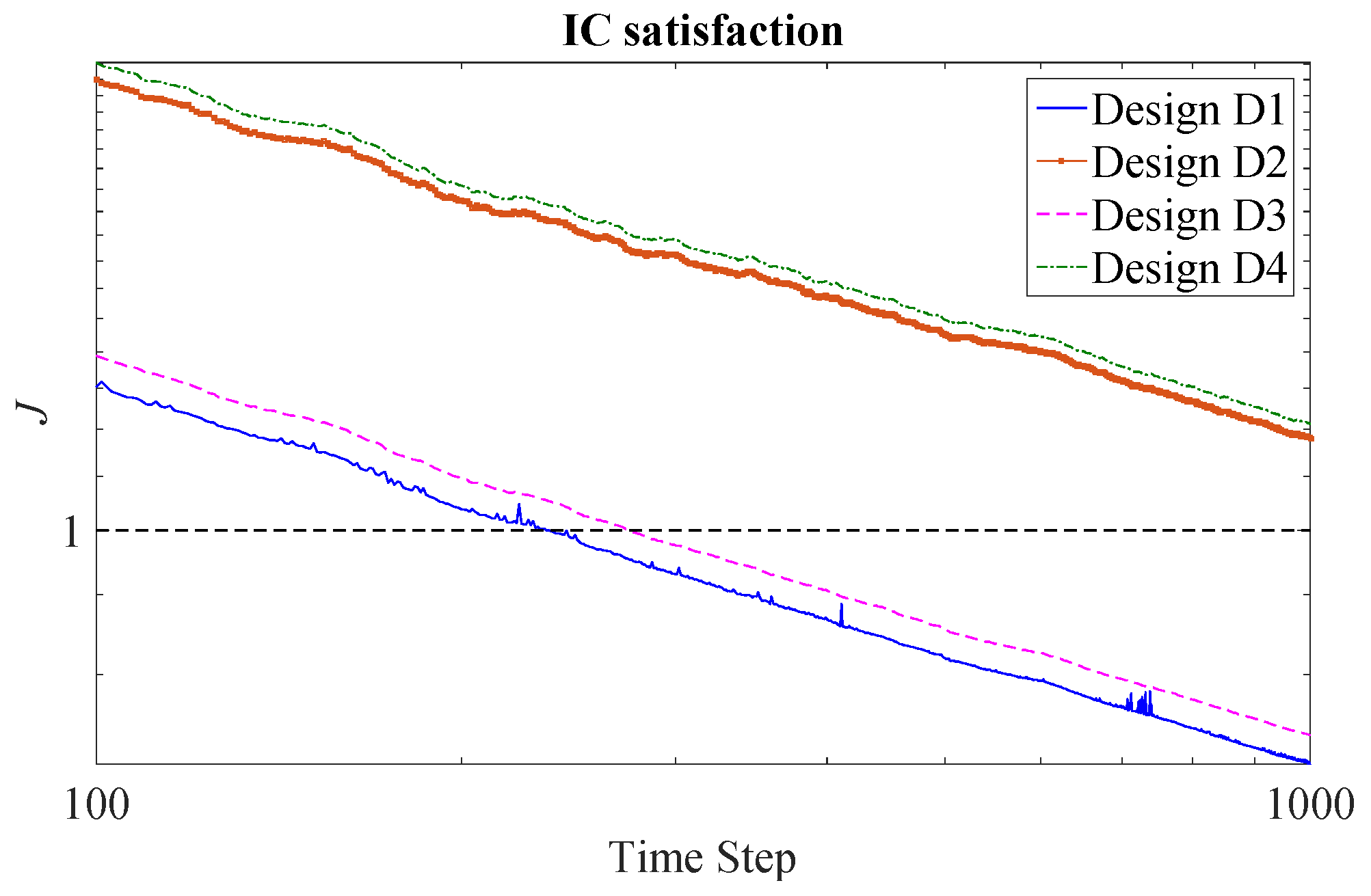
Figure 9.
Identification time required for satisfaction of IC for an FCC reactor-regenerator system when inputs are produced from designs D1–D4. (Equation (41)) for D1 and D3; (Equation (21)) for D2 and D4.
Figure 9.
Identification time required for satisfaction of IC for an FCC reactor-regenerator system when inputs are produced from designs D1–D4. (Equation (41)) for D1 and D3; (Equation (21)) for D2 and D4.
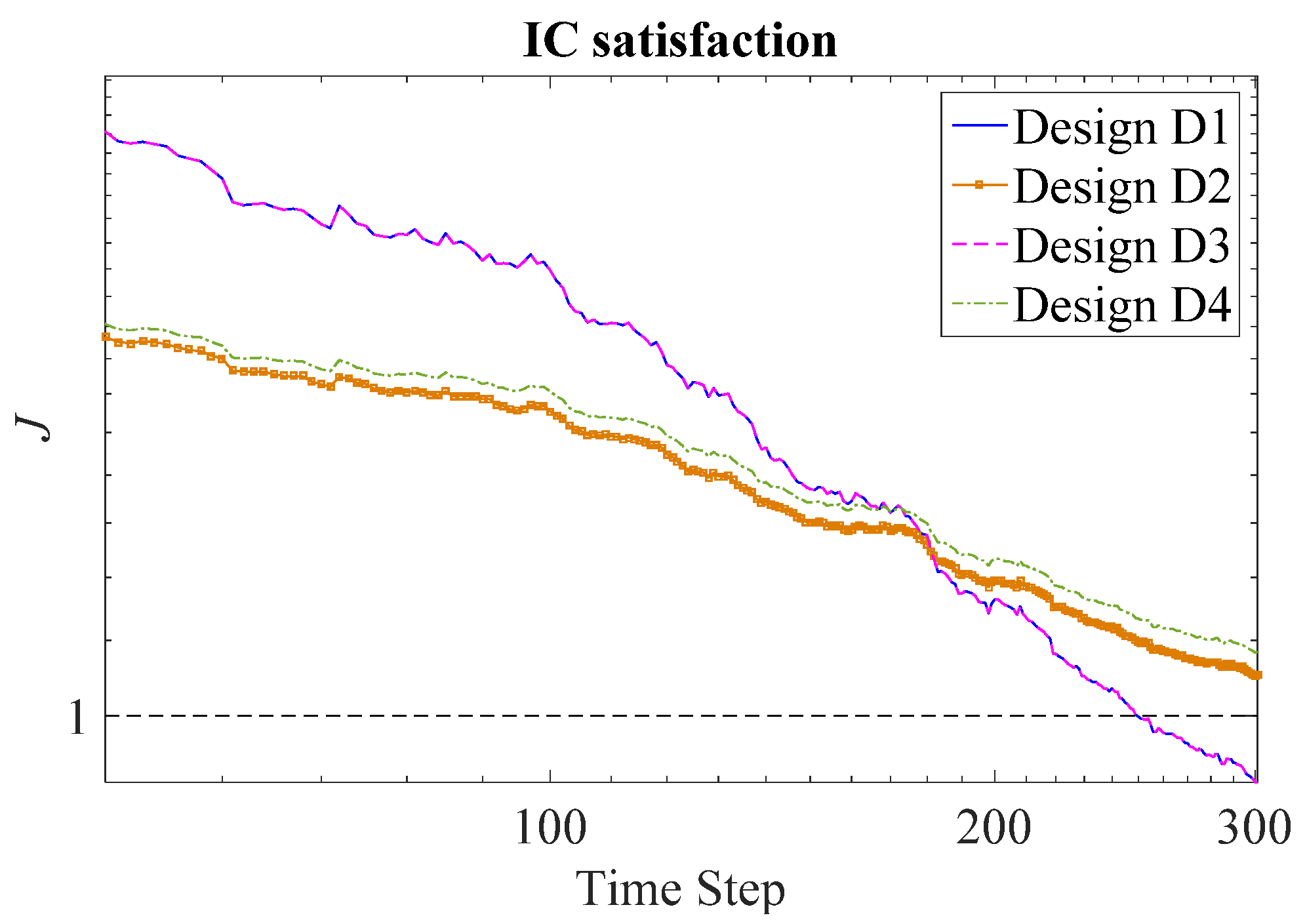
Figure 10.
Identification time required for satisfaction of IC for a two-stage absorber when inputs are produced from designs D1–D4. (Equation (44)) for D1 and D3; (Equation (21)) for D2 and D4.
Figure 10.
Identification time required for satisfaction of IC for a two-stage absorber when inputs are produced from designs D1–D4. (Equation (44)) for D1 and D3; (Equation (21)) for D2 and D4.
Table 1.
100-experiment averages for the design via Equation (26) on ; .
Table 1.
100-experiment averages for the design via Equation (26) on ; .
| Case | | | | |
|---|
| 142 | 0.9999 | −0.0023 | 2.63 × 10⁻¹² |
| 5.2 | 0.9292 | 0.9826 | 1.40 × 10⁻¹⁰ |
Table 2.
Summary of designs tested on and .
Table 2.
Summary of designs tested on and .
| Design | Objective | Constraints |
|---|
| ICmin | | Equation (32), triangular |
| Dmax | | Equation (32), |
| PRBSmax | | Equation (32) |
| ξmax | | Equation (32), , |
Table 3.
Summary of results for experiment designs on and . Corresponding variance value at its bound (active constraint in Equation (32)) is shown in bold and italics. Notation: , , : covariance matrices of , , , respectively; ; : Equation (31).
Table 3.
Summary of results for experiment designs on and . Corresponding variance value at its bound (active constraint in Equation (32)) is shown in bold and italics. Notation: , , : covariance matrices of , , , respectively; ; : Equation (31).
| | # | Bounds | Design | | | | | | | | | | | | | |
|---|
| Ill-conditioned column, G1 | 1 | | ICmin | 1.206 | 6.63 × 10⁻⁵ | 222 | 0.92 | 0.91 | 0.90 | 5.0 | −0.07 | 1.0 | 6.4 × 10⁻⁵ | 7.1 × 10⁻³ | 1.8 | 0.99996 |
| 2 | Dmax | 1.207 | 6.64 × 10⁻⁵ | 218 | 0.90 | 0.89 | 0.88 | 5.0 | 0.0 | 1.0 | 6.6 × 10⁻⁵ | 7.1 × 10⁻³ | 1.8 × 10⁻⁵ | 0.99996 |
| 3 | PRBSmax | 7.014 | 1.78 × 10⁻⁹ | 1.01 | 4.3 × 10⁻⁵ | 0.0 | 4.2 × 10⁻⁵ | 0.64 | 0.80 | 1.0 | 4.2 × 10⁻⁵ | 5.4 × 10⁻⁷ | 4.2 × 10⁻⁵ | 0.00000 |
| 4 | ξmax | 1.562 | 1.33 × 10⁻⁵ | 142 | 0.26 | 0.26 | 0.26 | 1.0 | 0.0 | 1.0 | 2.6 × 10⁻⁵ | 0.0 | 5.2 × 10⁻¹ | 0.99990 |
| 5 | | ICmin | 1.305 | 6.08 × 10⁻⁵ | 38.3 | 0.15 | 0.15 | 0.15 | 3.5 | 3.6 | 5.0 | 2.0 × 10⁻⁴ | 2.0 × 10⁻⁴ | 0.30 | 0.99864 |
| 6 | Dmax | 1.321 | 6.24 × 10⁻⁵ | 37.5 | 0.15 | 0.15 | 0.15 | 4.1 | 3.9 | 5.0 | 2.2 × 10⁻⁴ | 1.5 × 10⁻³ | 0.30 | 0.99858 |
| 7 | PRBSmax | 4.691 | 4.44 × 10⁻⁸ | 1.01 | 2.1 × 10⁻⁴ | 0.0 | 2.1 × 10⁻⁴ | 3.2 | 4.0 | 5.0 | 2.1 × 10⁻⁴ | 2.7 × 10⁻⁶ | 2.1 × 10⁻⁴ | 0.00000 |
| 8 | ξmax | 2.051 | 4.47 × 10⁻⁶ | 142 | 0.15 | 0.15 | 0.15 | 0.58 | 0.0 | 0.58 | 1.5 × 10⁻⁵ | 0.0 | 0.30 | 0.99990 |
| Well-conditioned column, G2 | 9 | | ICmin | 3.774 | 2.80 × 10⁻¹¹ | 1.67 | 4.0 × 10⁻⁶ | 2.0 × 10⁻⁶ | 8.0 × 10⁻⁶ | 1.1 | 1.0 | 1.1 | 4.8 × 10⁻⁶ | −2.6 × 10⁻⁶ | 7.2 × 10⁻⁶ | 0.35527 |
| 10 | Dmax | 3.984 | 3.20 × 10⁻¹¹ | 1.41 | 4.0 × 10⁻⁶ | 0.0 | 8.0 × 10⁻⁶ | 1.6 | 1.4 | 1.3 | 6.7 × 10⁻⁶ | −1.9 × 10⁻⁶ | 5.3 × 10⁻⁶ | 0.00000 |
| 11 | PRBSmax | 3.984 | 3.20 × 10⁻¹¹ | 1.41 | 4.0 × 10⁻⁶ | 0.0 | 8.0 × 10⁻⁶ | 1.6 | 1.4 | 1.3 | 6.7 × 10⁻⁶ | −1.9 × 10⁻⁶ | 5.3 × 10⁻⁶ | 0.00000 |
| 12 | ξmax | 6.327 | 8.07 × 10⁻¹³ | 6.54 | 4.0 × 10⁻⁶ | 2.7 × 10⁻⁶ | 2.0 × 10⁻⁶ | 5.9 × 10⁻² | 0.0 | 5.9 × 10⁻² | 1.4 × 10⁻⁷ | 0.0 | 5.9 × 10⁻⁶ | 0.94848 |
| 13 | | ICmin | 1.514 | 2.99 × 10⁻¹⁰ | 4.70 | 5.0 × 10⁻⁵ | 3.8 × 10⁻⁵ | 3.5 × 10⁻⁵ | 1.0 | 0.56 | 1.6 | 4.2 × 10⁻⁶ | −6.1 × 10⁻⁶ | 8.1 × 10⁻⁵ | 0.91026 |
| 14 | Dmax | 1.532 | 3.32 × 10⁻¹⁰ | 4.73 | 5.0 × 10⁻⁵ | 4.1 × 10⁻⁵ | 4.0 × 10⁻⁵ | 1.0 | 0.75 | 2.0 | 5.0 × 10⁻⁶ | −9.6 × 10⁻⁶ | 8.5 × 10⁻⁵ | 0.91350 |
| 15 | PRBSmax | 4.443 | 1.50 × 10⁻¹¹ | 1.11 | 4.3 × 10⁻⁶ | 0.0 | 3.5 × 10⁻⁶ | 1.0 | 0.77 | 0.66 | 3.8 × 10⁻⁶ | 3.7 × 10⁻⁷ | 4.0 × 10⁻⁶ | 0.00000 |
| 16 | ξmax | 1.789 | 1.26 × 10⁻¹⁰ | 6.54 | 5.0 × 10⁻⁵ | 3.4 × 10⁻⁵ | 2.5 × 10⁻⁵ | 0.74 | 0.0 | 0.74 | 1.7 × 10⁻⁶ | 0.0 | 7.3 × 10⁻⁵ | 0.94848 |
Table 4.
Skogestad and Morari column, . Results for different experiment designs. Generalized binary noise (GBN) signals in D3 and D4 are based on switching probability, , and mean switching time, . Active constraints are shown in bold italics.
Table 4.
Skogestad and Morari column, . Results for different experiment designs. Generalized binary noise (GBN) signals in D3 and D4 are based on switching probability, , and mean switching time, . Active constraints are shown in bold italics.
| Design | | | | | | | |
|---|
| D1 s.t. Equation (50) | 3.968 | 1.081 × 10⁻⁴ | 0.738 | 0.736 | 1.00 | 1.00 | 0.99990 |
| D2 s.t. Equation (50) | 3.968 | 1.081 × 10⁻⁴ | 0.738 | 0.736 | 1.00 | 1.00 | 0.99990 |
| D3 s.t. Equation (50) | 221.2 | 1.447 × 10⁻⁸ | 1.218 × 10⁻⁴ | 1.187 × 10⁻⁴ | 0.64 | 1.00 | 0.00000 |
| D4 s.t. Equation (50) | 3.968 | 1.081 × 10⁻⁴ | 0.738 | 0.736 | 1.00 | 1.00 | 0.99990 |
Table 5.
Wood and Berry column, . Results for different experiment designs. GBN signals in D3 and D4 are based on switching probability, , and mean switching time, . Active constraints are shown in bold italics.
Table 5.
Wood and Berry column, . Results for different experiment designs. GBN signals in D3 and D4 are based on switching probability, , and mean switching time, . Active constraints are shown in bold italics.
| Design | | | | | | | |
|---|
| D1 s.t. Equation (52) | 4.087 | 5.458 × 10⁻⁴ | 1.260 × 10⁻¹ | 2.851 × 10⁻² | 2.00 | 1.00 | 0.92087 |
| D2 s.t. Equation (52) | 4.078 | 5.426 × 10⁻⁴ | 1.342 × 10⁻¹ | 3.064 × 10⁻² | 2.00 | 1.00 | 0.93171 |
| D3 s.t. Equation (52) | 10.104 | 7.322 × 10⁻⁵ | 2.332 × 10⁻² | 3.140 × 10⁻³ | 1.872 | 1.00 | 0.00000 |
| D4 s.t. Equation (52) | 4.531 | 3.192 × 10⁻⁴ | 1.060 × 10⁻¹ | 2.998 × 10⁻² | 1.202 | 1.00 | 0.94848 |
Table 6.
FCC reactor-regenerator system. Results for different experiment designs. GBN signals in D3 are based on switching probability, , and mean switching time, . Active constraints are shown in bold italics.
Table 6.
FCC reactor-regenerator system. Results for different experiment designs. GBN signals in D3 are based on switching probability, , and mean switching time, . Active constraints are shown in bold italics.
| Design | | | , | , | |
|---|
| D1 s.t. Equation (54) | 94.42 | 0.985 | 1.50, 0.45, 3.00, 1.50, 1.25 | 0.16, 0.65, 0.35, 0.10, 0.21 | 0.70 |
| D2 s.t. Equation (54) | 90.47 | 0.791 | 1.50, 0.41, 3.00, 1.50, 1.21 | 0.16, 0.59, 0.35, 0.08, 0.20 | 0.75 |
| D3 s.t. Equation (54) | 144.2 | 0.026 | 1.07, 0.07, 0.62, 1.50, 0.35 | 0.12, 0.14, 0.35, 0.03, 0.06 | 0.00 |
Table 7.
Characterization of inputs and outputs for designs D1–D4 for a FCC unit; active constraints are in bold.
Table 7.
Characterization of inputs and outputs for designs D1–D4 for a FCC unit; active constraints are in bold.
| Design | | , | , | , |
|---|
| D1 | | | | |
| D2 | | | | |
| D3 | | | | |
| D4 | | | | |
Table 8.
Input and output correlations matrices for designs D1–D4 for a FCC unit.
Table 8.
Input and output correlations matrices for designs D1–D4 for a FCC unit.
| Design | | |
|---|
| D1 | | |
| D2 | | |
| D3 | | |
| D4 | | |
Table 9.
Characterization of inputs and outputs designs D1–D4 for a two-stage absorber; active constraints are in bold.
Table 9.
Characterization of inputs and outputs designs D1–D4 for a two-stage absorber; active constraints are in bold.
| Design | | | | | | |
|---|
| D1 | | | | | | |
| D2 | | | | | | |
| D3 | | | | | | |
| D4 | | | | | | |


