
Using a One-Dimensional Convolutional Neural Network with Taguchi Parametric Optimization for a Permanent-Magnet Synchronous Motor Fault-Diagnosis System


Abstract
:1. Introduction
2. Materials and Methods
2.1. Taguchi Method
2.1.1. Analysis of Average Value
2.1.2. Analysis of Variance
2.2. Materials
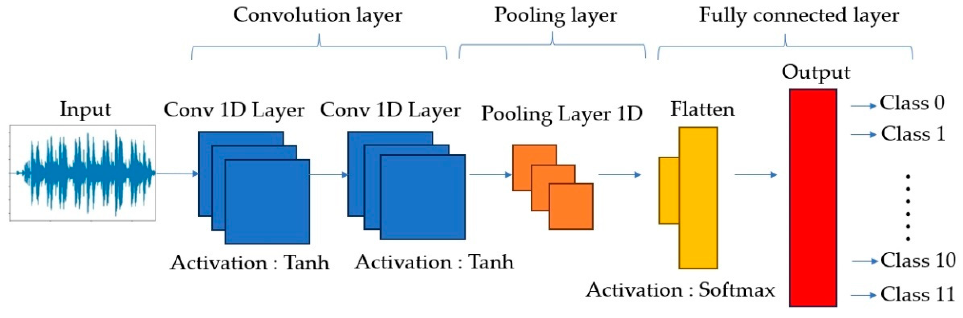
2.3. One-Dimensional CNN
2.3.1. Convolution Layer
2.3.2. Pooling Layer
2.3.3. Fully Connected Layer
3. Experimental Results
3.1. Taguchi Method
3.2. Design of Taguchi Single-Objective Optimization
3.2.1. Average Value Analysis of Recognition Accuracy
3.2.2. Average Value Analysis of Loss Function
3.2.3. Analysis of Taguchi Single-Objective Optimization Results
3.3. The Multi-Objective Optimization Design
4. Discussion
5. Conclusions
Author Contributions
Funding
Data Availability Statement
Conflicts of Interest
References
- Jeong, Y.S.; Sul, S.K.; Schulz, S.E. Fault detection and fault-tolerant control of interior permanent-magnet motor drive system for electric vehicle. IEEE Trans. Ind. Appl. 2005, 41, 46–51. [Google Scholar] [CrossRef]
- Ionel, D.M.; Popescu, M. Finite-Element Surrogate Model for Electric Machines with Revolving Field-Application to IPM Motors. IEEE Trans. Ind. Appl. 2010, 46, 2424–2433. [Google Scholar] [CrossRef]
- Zhao, A.M. Motor Fault Diagnosis by Using Fuzzy Neural Network. Master’s Thesis, Chung Yuan Christian University of Taiwan, Taoyuan City, Taiwan, 2004. [Google Scholar]
- Peng, S.T. Fault Diagnosis by Using Multiple Vibration Signals for Motors. Master’s Thesis, Chung Yuan Christian University of Taiwan, Taoyuan City, Taiwan, 2004. [Google Scholar]
- Huang, S.R.; Huang, K.H.; Chao, K.H.; Chiang, W.T. Fault analysis and diagnosis system for induction motors. Comput. Electr. Eng. 2016, 54, 195–209. [Google Scholar] [CrossRef]
- Athif, N.M.; Febriyanti, S.; Ramadhan, K.N. Face Mask Detection under Low Light Condition Using Convolutional Neural Network (CNN). J. Ilm. Penelit. Dan Pembelajaran Inform. 2023, 8, 281–290. [Google Scholar] [CrossRef]
- Ding, M.H.; Ding, Y.P.; Peng, Y.Q.; Cao, J.X. CNN-Based Time–Frequency Image Enhancement Algorithm for Target Tracking Using Doppler Through-Wall Radar. IEEE Geosci. Remote Sens. Lett. 2023, 20, 3505305. [Google Scholar] [CrossRef]
- Meng, Z.; Cao, W.; Sun, D.Y.; Li, Q.; Ma, W.X.; Fan, F.J. Research on fault diagnosis method of MS-CNN rolling bearing based on local central moment discrepancy. Adv. Eng. Inform. 2022, 54, 101797. [Google Scholar] [CrossRef]
- Xu, S.W.; Ru, H.T.; Li, D.C.; Shui, P.L.; Jian, X. Marine Radar Small Target Classification Based on Block-Whitened Time–Frequency Spectrogram and Pre-Trained CNN. IEEE Trans. Geosci. Remote Sens. 2023, 61, 5101311. [Google Scholar] [CrossRef]
- Ribeiro, R.F., Jr.; Methodoly, I.; Campos, M.; Teixeira, C.; Silva, L.; Gomes, G. Fault detection and diagnosis in electric motors using 1d convolutional neural networks with multi-channel vibration signals. Measurement 2022, 190, 110759. [Google Scholar]
- Rajagopalan, S.; Singh, J.; Purohit, A. Performance analysis of genetically optimized 1D-convolutional neural network architecture for rotor system fault detection and diagnosis. Proc. Inst. Mech. Eng. Part E J. Process Mech. Eng. 2024, 10, 1177. [Google Scholar] [CrossRef]
- Gu, Y.; Zhang, Y.J.; Yang, M.R.; Li, C.S. Motor On-Line Fault Diagnosis Method Research Based on 1D-CNN and Multi-Sensor Information. Appl. Sci. 2023, 13, 4192. [Google Scholar] [CrossRef]
- Saufi, M.S.R.M.; Muhammad, F.B.I.; Talib, H.; Zain, M.Z.M. Extremely Low-Speed Bearing Fault Diagnosis Based on Raw Signal Fusion and DE-1D-CNN Network. J. Vib. Eng. Technol. 2023, 10, 1007. [Google Scholar]
- Xie, T.; Zhang, W.D.; Zhang, Y.B.; Ahmed, Z.; Tang, Y.F. Marine Current Turbine Multi-Fault Diagnosis based on Optimization Resampled Modulus Feature and 1D-CNN. IEEE Trans. Instrum. Measurement. 2023, 72, 3515910. [Google Scholar] [CrossRef]
- He, J.; Li, X.; Chen, Y. Deep Transfer Learning Method Based on 1D-CNN for Bearing Fault Diagnosis. Shock Vib. 2021, 2021, 6687331. [Google Scholar] [CrossRef]
- Canel, T.; Zeren, M.; Sınmazçelik, T. Laser parameters optimization of surface treating of Al 6082-T6 with Taguchi method. Opt. Laser Technol. 2019, 120, 105714. [Google Scholar] [CrossRef]
- Sachin, P. Parameter Optimization of Turning Process (Cast Iron) Using Taguchi Method. Int. J. Eng. Res. Technol. 2023, 3, 2525–2529. [Google Scholar]
- Srikanth, V.; Leela, B.; Sai, M. Optimization of Machining Parameters for Mild Steel in Dry Turning Using Taguchi Method. Int. J. Sci. Res. Eng. Manag. 2023, 7, 1–11. [Google Scholar] [CrossRef]
- Lin, C.J.; Lin, C.J.; Lin, X.Q. Automatic Sleep Stage Classification Using a Taguchi-Based Multiscale Convolutional Compensatory Fuzzy Neural Network. Appl. Sci. 2023, 13, 10442. [Google Scholar] [CrossRef]
- Mohammed, Y.; Mohammed, A.S. A Statistical Analysis of Joint Strength of dissimilar Aluminum Alloys Formed by Friction Stir Welding using Taguchi Design Approach, ANOVA for the Optimization of Process Parameters. Int. J. Res. Eng. Technol. 2015, 3, 61–68. [Google Scholar]
- Özel, S.; Vural, E.; Binici, M. Optimization of the effect of thermal barrier coating (TBC) on diesel engine performance by Taguchi method. Fuel 2020, 263, 116537. [Google Scholar] [CrossRef]
- Kim, S.I.; Lee, J.Y.; Hong, J.P.; Hur, Y.; Jung, Y.H. Optimization for Reduction of Torque Ripple in Interior Permanent Magnet Motor by Using the Taguchi Method. IEEE Trans. Magn. 2005, 41, 1796–1799. [Google Scholar]
- Zhu, W.J.; Yang, X.Y.; Lan, Z.Y. Structure Optimization Design of High-Speed BLDC Motor Using Taguchi Method. In Proceedings of the 2010 International Conference on Electrical and Control Engineering (ICECE), Wuhan, China, 25–27 June 2010; pp. 4247–4249. [Google Scholar]
- Huang, S.-R.; Huang, K.-H. Multi-Objective Optimization Design of Variable-Frequency Induction Motor for Ceiling Fans Using Response Surface Methodology. ICIC Express Lett. Part B Appl. 2016, 7, 679–686. [Google Scholar]
- Hammad, M.; Iliyasu, A.M.; Subasi, A.; Ho, E.S.L.; El-Latif, A.A.A. A Multitier Deep Learning Model for Arrhythmia Detection. IEEE Trans. Instrum. Meas. 2021, 70, 3033072. [Google Scholar] [CrossRef]
- Lin, C.J.; Jeng, S.Y.; Chen, M.K. Using 2D CNN with Taguchi Parametric Optimization for Lung Cancer Recognition from CT Images. Appl. Sci. 2020, 10, 2591. [Google Scholar] [CrossRef]
- Rezania, A.; Atouei, S.A.; Rosendahl, L. Critical parameters in integration of thermoelectric generators and phase change materials by numerical and Taguchi methods. Mater. Today Energy 2020, 16, 100376. [Google Scholar] [CrossRef]
- Ishaq, M.; Khan, M.; Kwon, S. TC-Net: A Modest & Lightweight Emotion Recognition System Using Temporal Convolution Network. Comput. Syst. Sci. Eng. 2023, 46, 3355–3369. [Google Scholar]
- Idris, F.N.; Nadzir, M.M.; Shukor, S.R.A. Optimization of solvent-free microwave extraction of Centella asiatica using Taguchi method. J. Environ. Chem. Eng. 2020, 8, 103766. [Google Scholar] [CrossRef]
- Trigueros, D.S.; Meng, L.; Hartnett, M. Enhancing convolutional neural networks for face recognition with occlusion maps and batch triplet loss. Image Vis. Comput. 2018, 79, 99–108. [Google Scholar] [CrossRef]
- Giménez, M.; Palanca, J.; Botti, V. Semantic-based padding in convolutional neural networks for improving the performance in natural language processing. A case of study in sentiment analysis. Neurocomputing 2020, 378, 315–323. [Google Scholar] [CrossRef]
- Lu, S.D.; Wang, M.H.; Wei, S.E.; Liu, H.D.; Wu, C.C. Photovoltaic Module Fault Detection Based on a Convolutional Neural Network. Processes 2021, 9, 1635. [Google Scholar] [CrossRef]
- Lau, M.M.; Lim, K.H. Review of Adaptive Activation Function in Deep Neural Network. In Proceedings of the 2018 IEEE-EMBS Conference on Biomedical Engineering and Sciences (IECBES), Sarawak, Malaysia, 3–6 December 2018. [Google Scholar]
- Zeiler, M.D.; Fergus, R. Visualizing and Understanding Convolutional Networks. In Proceedings of the European Conference on Computer Vision, Zurich, Switzerland, 6–12 September 2014. [Google Scholar]


| No. | Control Factors | Level 1 | Level 2 | Level 3 |
|---|---|---|---|---|
| A | Pooling function | Max | Average | |
| B | Conv1_filters | 50 | 100 | 150 |
| C | Conv1_kernel size | 10 | 20 | 30 |
| D | Conv1_strides | 4 | 6 | 8 |
| E | Conv2_ filters | 10 | 20 | 30 |
| F | Conv2_ kernel size | 15 | 20 | 25 |
| G | Conv2_strides | 1 | 2 | 3 |
| Exp. No. | A | B | C | D | E | F | G |
|---|---|---|---|---|---|---|---|
| 1 | Max | 50 | 10 | 4 | 10 | 15 | 1 |
| 2 | Max | 50 | 20 | 6 | 20 | 20 | 2 |
| 3 | Max | 50 | 30 | 8 | 30 | 25 | 3 |
| 4 | Max | 100 | 10 | 4 | 20 | 20 | 3 |
| 5 | Max | 100 | 20 | 6 | 30 | 25 | 1 |
| 6 | Max | 100 | 30 | 8 | 10 | 15 | 2 |
| 7 | Max | 150 | 10 | 6 | 10 | 25 | 2 |
| 8 | Max | 150 | 20 | 8 | 20 | 15 | 3 |
| 9 | Max | 150 | 30 | 4 | 30 | 20 | 1 |
| 10 | Average | 50 | 10 | 8 | 30 | 20 | 2 |
| 11 | Average | 50 | 20 | 4 | 10 | 25 | 3 |
| 12 | Average | 50 | 30 | 6 | 20 | 15 | 1 |
| 13 | Average | 100 | 10 | 6 | 30 | 15 | 3 |
| 14 | Average | 100 | 20 | 8 | 10 | 20 | 1 |
| 15 | Average | 100 | 30 | 4 | 20 | 25 | 2 |
| 16 | Average | 150 | 10 | 8 | 20 | 25 | 1 |
| 17 | Average | 150 | 20 | 4 | 30 | 15 | 2 |
| 18 | Average | 150 | 30 | 6 | 10 | 20 | 3 |
| Item | Specification |
|---|---|
| Motor type | PMSM |
| Poles/slots | 4 poles/24 slots |
| Rated voltage | 311 VDC |
| Rated rpm | 2500 rpm |
| Rated power | 600 W |
| Phase | Three-phase |
| Construction of winding | Single-layer concentric winding |
| Connection | Y-connection |
| Bandwidth | 1578.5 Hz |
| Lines of resolution | 51,200 |
| Capture time | 32.4 s |
| Exp. No. | A | B | C | D | E | F | G | Acc. (%) | Loss | ACC. | Loss |
|---|---|---|---|---|---|---|---|---|---|---|---|
| 1 | Max | 50 | 10 | 4 | 10 | 15 | 1 | 98.68 | 0.0019 | 39.885 | 54.425 |
| 2 | Max | 50 | 20 | 6 | 20 | 20 | 2 | 99.84 | 0.00026 | 39.986 | 71.701 |
| 3 | Max | 50 | 30 | 8 | 30 | 25 | 3 | 98.94 | 0.0014 | 39.907 | 57.077 |
| 4 | Max | 100 | 10 | 4 | 20 | 20 | 3 | 99.71 | 0.00049 | 39.975 | 66.196 |
| 5 | Max | 100 | 20 | 6 | 30 | 25 | 1 | 99.71 | 0.00038 | 39.975 | 68.404 |
| 6 | Max | 100 | 30 | 8 | 10 | 15 | 2 | 98.98 | 0.0015 | 39.911 | 56.478 |
| 7 | Max | 150 | 10 | 6 | 10 | 25 | 2 | 97.63 | 0.0032 | 39.792 | 49.897 |
| 8 | Max | 150 | 20 | 8 | 20 | 15 | 3 | 99.29 | 0.00099 | 39.938 | 60.087 |
| 9 | Max | 150 | 30 | 4 | 30 | 20 | 1 | 99.43 | 0.00074 | 39.950 | 62.615 |
| 10 | Average | 50 | 10 | 8 | 30 | 20 | 2 | 99.04 | 0.0017 | 39.916 | 55.391 |
| 11 | Average | 50 | 20 | 4 | 10 | 25 | 3 | 95.08 | 0.0073 | 39.562 | 42.734 |
| 12 | Average | 50 | 30 | 6 | 20 | 15 | 1 | 98.28 | 0.0026 | 39.849 | 51.701 |
| 13 | Average | 100 | 10 | 6 | 30 | 15 | 3 | 99.40 | 0.001 | 39.948 | 60.000 |
| 14 | Average | 100 | 20 | 8 | 10 | 20 | 1 | 96.96 | 0.0046 | 39.732 | 46.745 |
| 15 | Average | 100 | 30 | 4 | 20 | 25 | 2 | 99.67 | 0.00062 | 39.971 | 64.152 |
| 16 | Average | 150 | 10 | 8 | 20 | 25 | 1 | 98.93 | 0.0016 | 39.907 | 55.918 |
| 17 | Average | 150 | 20 | 4 | 30 | 15 | 2 | 99.48 | 0.00074 | 39.955 | 62.615 |
| 18 | Average | 150 | 30 | 6 | 10 | 20 | 3 | 91.12 | 0.0119 | 39.192 | 38.489 |
| Level | A | B | C | D | E | F | G |
|---|---|---|---|---|---|---|---|
| 1 | 39.92 | 39.85 | 39.9 | 39.88 | 39.679 | 39.91 | 39.88 |
| 2 | 39.78 | 39.92 | 39.86 | 39.79 | 39.938 | 39.79 | 39.92 |
| 39.79 | 39.8 | 39.89 | 39.942 | 39.85 | 39.75 | ||
| Delta | 0.14 | 0.13 | 0.11 | 0.09 | 0.263 | 0.12 | 0.17 |
| Rank | 3 | 4 | 6 | 7 | 1 | 5 | 2 |
| Best parameter | Max Pooling | 100 | 10 | 8 | 30 | 15 | 2 |
| Level | A | B | C | D | E | F | G |
|---|---|---|---|---|---|---|---|
| 1 | 60.76 | 55.5 | 56.97 | 58.79 | 48.13 | 57.55 | 56.63 |
| 2 | 53.08 | 60.33 | 58.71 | 56.7 | 61.63 | 56.86 | 60.04 |
| 3 | 54.94 | 55.09 | 55.28 | 61.02 | 56.36 | 54.1 | |
| Delta | 7.68 | 5.39 | 3.63 | 3.51 | 13.5 | 1.19 | 5.94 |
| Rank | 2 | 4 | 5 | 6 | 1 | 7 | 3 |
| Best parameter | Max Pooling | 100 | 20 | 4 | 20 | 15 | 2 |
| Object | A | B | C | D | E | F | G | Acc. (%) | Loss |
|---|---|---|---|---|---|---|---|---|---|
| Acc. | Max | 100 | 10 | 8 | 30 | 15 | 2 | 99.86 | 0.00027 |
| Loss | Max | 100 | 20 | 4 | 20 | 15 | 2 | 99.86 | 0.00024 |
| Factors | Accuracy | Loss | ||||
|---|---|---|---|---|---|---|
| Degree of Freedom | Sum of Squares | Effect (%) | Degree of Freedom | Sum of Squares | Effect (%) | |
| A | 1 | 0.09202 | 14.13 | 1 | 265.55 | 20.37 |
| B | 2 | 0.05043 | 7.74 | 2 | 105.35 | 8.08 |
| C | 2 | 0.03436 | 5.27 | 2 | 39.53 | 3.03 |
| D | 2 | 0.03517 | 5.40 | 2 | 37.35 | 2.86 |
| E | 2 | 0.27239 | 41.82 | 2 | 697.39 | 53.48 |
| F | 2 | 0.04488 | 6.89 | 2 | 4.27 | 0.33 |
| G | 2 | 0.09296 | 14.27 | 2 | 106.67 | 8.18 |
| Error | 4 | 0.0292 | 4.48 | 4 | 47.83 | 3.67 |
| Sum | 17 | 0.6514 | 100% | 17 | 1303.94 | 100% |
| Object | A | B | C | D | E | F | G | Acc. (%) | Loss |
|---|---|---|---|---|---|---|---|---|---|
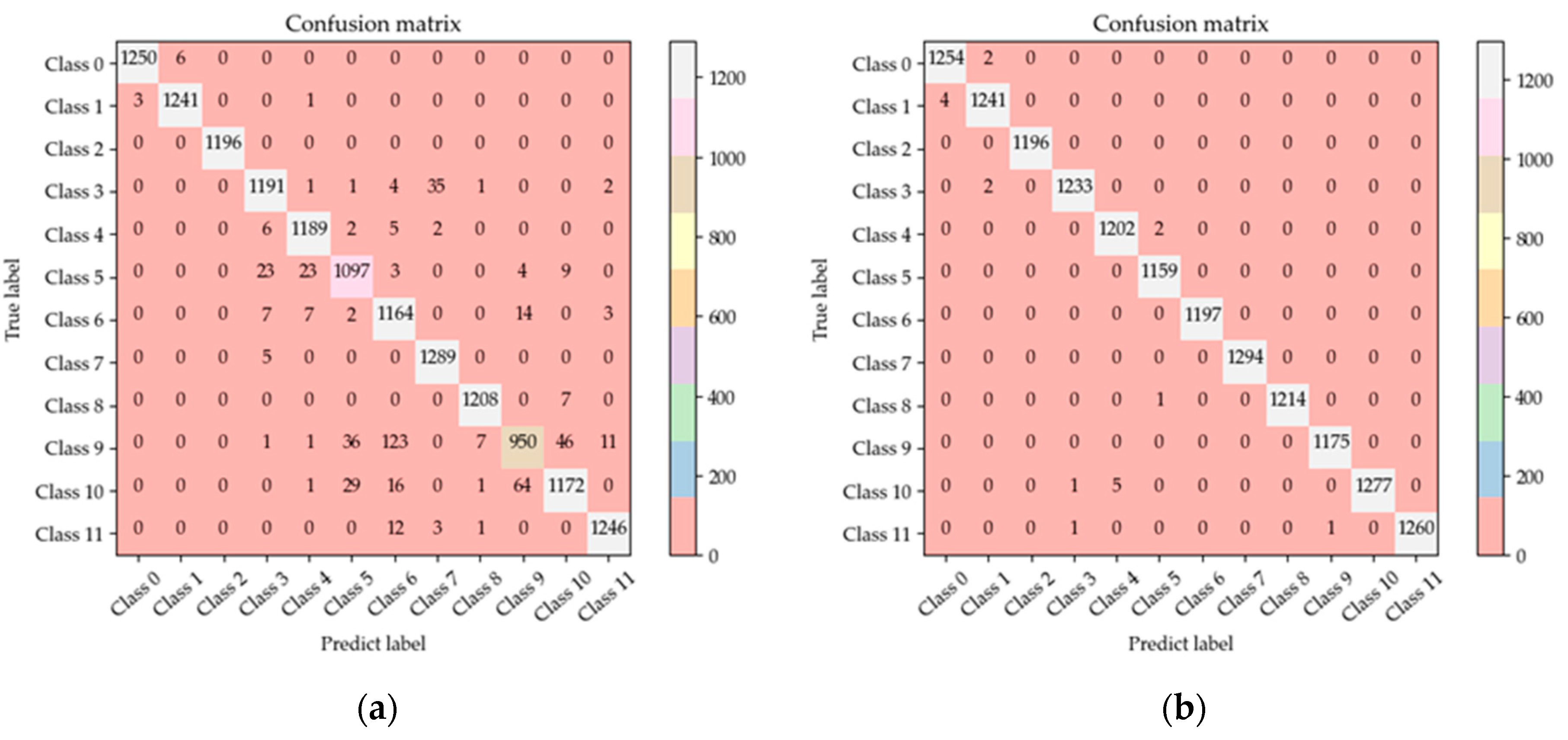
| Taguchi+ ANOVA | Max | 100 | 10 | 8 | 20 | 15 | 2 | 99.91 | 0.00011 |
| Original | Max | 50 | 20 | 4 | 10 | 25 | 3 | 96.75 | 0.0045 |
| Epoch | Accuracy Rate (%) | Loss | Rank | |
|---|---|---|---|---|
| 1D CNN with Taguchi and ANOVA | 50 | 99.91 | 0.00011 | 1 |
| 1D CNN with Taguchi (Loss) | 50 | 99.86 | 0.00024 | 2 |
| 1D CNN with Taguchi (Accuracy rate) | 50 | 99.86 | 0.00027 | 3 |
| Original 1D CNN | 50 | 96.75 | 0.0045 | 4 |
| 2D CNN | 50 | 96.1 | 0.0075 | 5 |
Disclaimer/Publisher’s Note: The statements, opinions and data contained in all publications are solely those of the individual author(s) and contributor(s) and not of MDPI and/or the editor(s). MDPI and/or the editor(s) disclaim responsibility for any injury to people or property resulting from any ideas, methods, instructions or products referred to in the content. |
© 2024 by the authors. Licensee MDPI, Basel, Switzerland. This article is an open access article distributed under the terms and conditions of the Creative Commons Attribution (CC BY) license (https://creativecommons.org/licenses/by/4.0/).
Share and Cite
Wang, M.-H.; Chan, F.-C.; Lu, S.-D. Using a One-Dimensional Convolutional Neural Network with Taguchi Parametric Optimization for a Permanent-Magnet Synchronous Motor Fault-Diagnosis System. Processes 2024, 12, 860. https://doi.org/10.3390/pr12050860
Wang M-H, Chan F-C, Lu S-D. Using a One-Dimensional Convolutional Neural Network with Taguchi Parametric Optimization for a Permanent-Magnet Synchronous Motor Fault-Diagnosis System. Processes. 2024; 12(5):860. https://doi.org/10.3390/pr12050860
Chicago/Turabian StyleWang, Meng-Hui, Fu-Chieh Chan, and Shiue-Der Lu. 2024. "Using a One-Dimensional Convolutional Neural Network with Taguchi Parametric Optimization for a Permanent-Magnet Synchronous Motor Fault-Diagnosis System" Processes 12, no. 5: 860. https://doi.org/10.3390/pr12050860