Production Capacity Prediction and Optimization in the Glycerin Purification Process: A Simulation-Assisted Few-Shot Learning Approach

Abstract

Chemical process control relies on a tightly controlled, narrow range of margins for critical variables, ensuring process stability and safeguarding equipment from potential accidents. The availability of historical process data is limited to a specific setpoint of operation. This challenge raises issues for process monitoring in predicting and adjusting to deviations outside of the range of operational parameters. Therefore, this paper proposes simulation-assisted deep transfer learning for predicting and optimizing the final purity and production capacity of the glycerin purification process. The proposed network is trained by the simulation domain to generate a base feature extractor, which is then fine-tuned using few-shot learning techniques on the target learner to extend the working domain of the model beyond historical practice. The result shows that the proposed model improved prediction performance by 24.22% in predicting water content and 79.72% in glycerin prediction over the conventional deep learning model. Additionally, the implementation of the proposed model identified production and product quality improvements for enhancing the glycerin purification process.

1. Introduction

Biodiesel, a renewable energy source, is gaining prominence as the world seeks sustainable alternatives to fossil fuels. Its production, derived from natural sources such as vegetable oils, animal fats, and recycled greases, has grown significantly in recent years [1]. This increase is primarily driven by global commitments against climate change and the push towards greener energy sources. The production process of biodiesel involves transesterification, where fats and oils are converted into fatty acid methyl esters. An often-overlooked by-product of biodiesel production is glycerin. For every ten pounds of biodiesel produced, approximately one pound of glycerin is generated [2]. Despite being a by-product, glycerin holds immense value in various industries. However, the glycerin produced typically contains impurities and contaminants, necessitating purification to meet quality standards. This purification process, which removes unwanted substances such as water and fatty acids, faces challenges due to a limited operating domain and a narrow control range. These constraints hinder its ability to effectively and efficiently remove the wide array of impurities found in glycerin by-products from biodiesel production, posing a significant challenge in consistently producing high-quality glycerin [3].

Accurately predicting process efficiency is crucial, especially under operating conditions that extend beyond the standard monitoring range. This complexity raises challenges in determining controller actions to compensate for process disturbances while ensuring the desired product quality is maintained [4]. A prime example is observed in glycerin purification. Critical factors such as the composition of the feed stream, the water-to-glycerin ratio, the performance of the evaporation unit, and adjustments to manipulated variables in the distillation column must be meticulously managed. These adjustments are necessary not only to maintain the quality of refined glycerin but also to ensure that the controller actions are effective within the unit operation constraints.

Expert engineers frequently modify these conditions, relying on their specialized knowledge and on-site experimental data [5]. However, the limited scope of most operating variables can often hamper the efficiency of glycerin purification. The complexity of the process increases due to the multitude of variables influencing operating conditions, which can lead to process instability [6]. Consequently, this challenge has led researchers to turn their focus toward utilizing artificial intelligence (AI) and data-driven techniques [7]. These methods offer the ability to analyze large datasets, identify patterns, and make predictions or real-time decisions using the information provided [8]. Even if the prediction skill of the AI-based method is high, the result can be deviated by multiple characteristics of process operation [9].

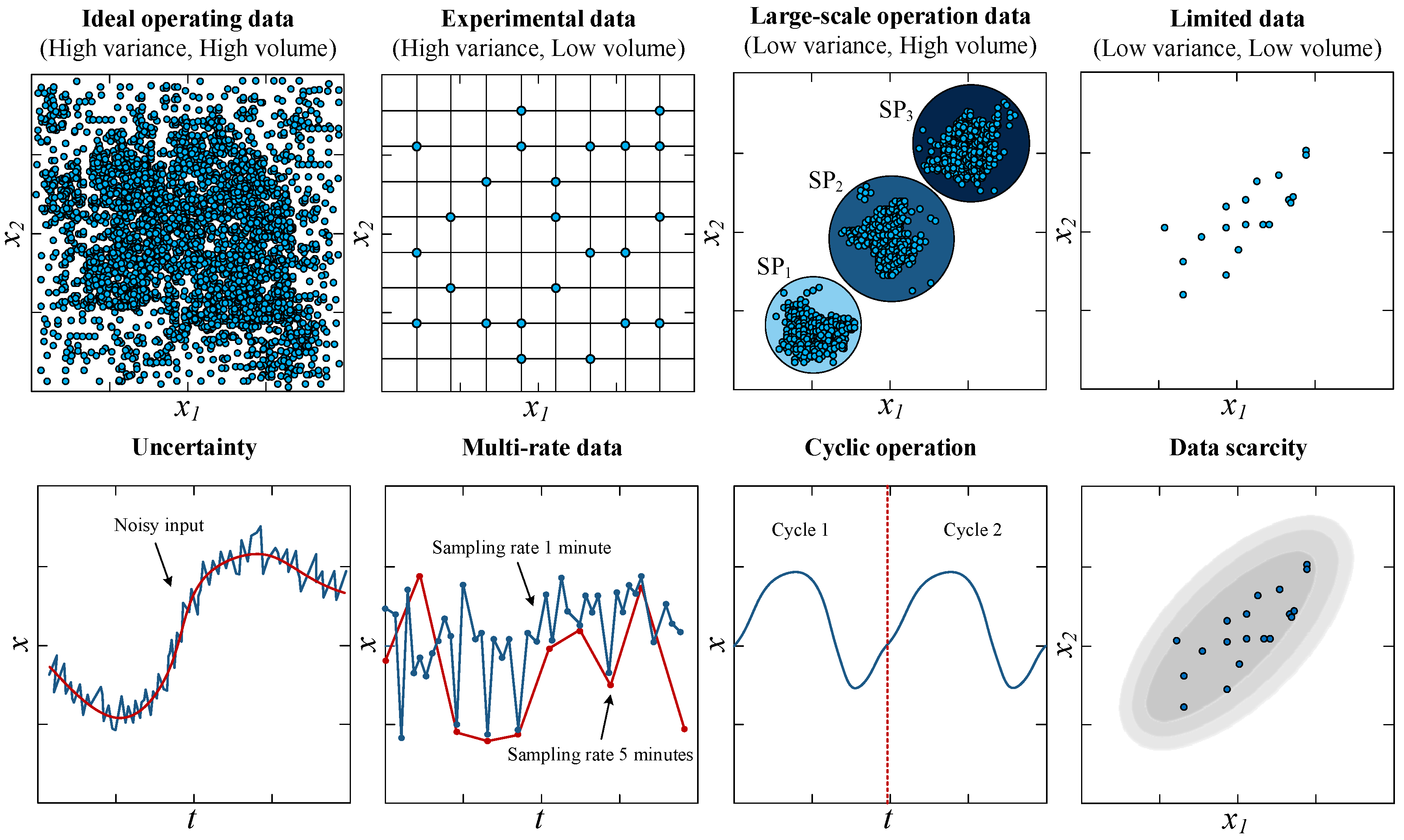
In chemical process optimization, data can be categorized by two criteria: variance/volume tradeoff and challenges from the data characteristics, as illustrated in Figure 1. In the case of the variance/volume tradeoff, the ‘Large-scale operation data’ exemplify a limited operating domain, with datapoints predominantly clustered around the setpoint, indicating a narrow focus on operational conditions under normal circumstances with high volume and low variance. Conversely, the ‘Limited data’ represent a limited amount of data, with sparse datapoints reflecting rare yet significant operational states that are critical to process stability and quality. The dearth of data in both cases—the limited operating domain and the limited number of available datapoints—not only poses substantial challenges for process monitoring and control, especially when it comes to adapting to and managing deviations that fall outside the usual operational parameters, but also makes the prediction model unreliable outside the experienced domain. On the other hand, when considering challenges from data characteristics, four commonly found problems are uncertainty, multi-rate information, cyclic operation, and limited data [10].

Researchers have proposed multiple innovative techniques to resolve these challenges. Regarding uncertainty, Panjapornpon et al. introduced a deep learning model constructed using a compensation architecture for energy optimization that addresses measurement uncertainties [11]. Similarly, Wiebe, Cecilo, and Misener integrated data-driven stochastic degradation models with optimization strategies, using robust techniques to manage uncertainties in equipment degradation. Lastly, Moghadasi et al. proposed a gradient-boosting machine with the density-based spatial clustering of applications with noise to optimize steam consumption in the gas sweetening process [12]. These contributions show that the advancement of the data-driven method can be significantly useful in resolving the challenges facing industrial processes. However, a common thread among these techniques is their reliance on large datasets. The integration of data cleaning methods and network architecture modification can remove the contribution made by process disturbances, but it requires a lot of training information, as well as careful tuning of the network parameters, to ensure that the resulting model accurately reflects the underlying system dynamics without being overly influenced by noise or irrelevant data [13]. This approach typically involves iterative refinement of both the data preprocessing steps and the network architecture to strike a balance between the model complexity and generalization ability [14].

When encountering complex scenarios such as in the chemical industry, the framework of the AI-based model may change according to the challenges that the research focuses on [15]. Han et al. proposed a feed-forward neural network (FNN) with data envelopment analysis (DEA) for the optimization of ethylene production [16]. The integration of DEA with a deep learning model can help in optimization, but based on its architecture, the network might not effectively capture all nonlinear relationships. This can be resolved using the recurrent neural network, such as long short-term memory (LSTM) [17]. The network has a recurrent interval state that helps in handling the long-term dependency found in the data [18]. The performance of the LSTM network can be enhanced by integrating with an attention mechanism (AM). AM-LSTM is particularly useful in tasks where the sequence is long and not equally important along the sequence, by allowing the network to weigh diverse parts of the input differently [19]. However, despite these advancements, AM-LSTM networks still face challenges in terms of adaptability and scalability, particularly when dealing with limited data scenarios, both in terms of quantity and domain-specific data. To resolve this issue, Han et al. proposed a hybrid approach using Monte Carlo (MC) simulation to expand the working domain of the LSTM network [20]. By simulating a wide range of possible scenarios, the MC-LSTM model can effectively deal with limited data situations. Since it provided an improvement, it is important to note that MC simulation is inherently probabilistic, relying solely on random sampling techniques. The integration of digital twin technology offers a more holistic and accurate simulation [21]. Digital twins create dynamic virtual representations of physical systems, allowing for more detailed and realistic scenario modeling while perfectly eliminating limited data problems [22]. Based on the aforementioned literature, an overview of research on AI applications in production capacity analysis is presented in

Table 1. Overview of research on production capacity optimization.

Reference	Year	Application	Method	Focus
				PO	LD
Geng et al. [23]	2018	Ethylene and PTA production	Extreme learning machine with interpretative structural modeling	✓
Han et al. [24]	2019	PTA solvent system	LSTM integrated with an attention mechanism	✓
Han et al. [25]	2019	Ethylene and PTA production	Extreme learning machine with affinity propagation	✓
Geng et al. [26]	2020	Ethylene process	Improved CNN based on cross feature	✓
Han et al. [20]	2023	Ethylene process	LSTM with Monte Carlo simulation	✓	✓

PO refers to production optimization, while LD denotes limited data challenges.

where several research gaps can be identified:

• Adaptability to limited and sparse data: Existing models, including advanced neural networks, often require large datasets for training. This necessity poses a challenge in scenarios where data are sparse or limited, as is common in chemical process optimization.
• Improvement beyond Monte Carlo simulations: While the MC-LSTM model represents an advancement in dealing with limited data scenarios, the reliance on probabilistic, random sampling techniques indicates a gap. Exploring alternatives or enhancements to Monte Carlo simulations that offer deterministic modeling approaches could provide more reliable and accurate predictions.
• Integration of digital twin technology: The introduction of digital twin technology for more accurate scenario modeling is a promising direction. However, the seamless integration of this technology with AI-based models, particularly in optimizing the chemical process and production capacity, remains a gap.

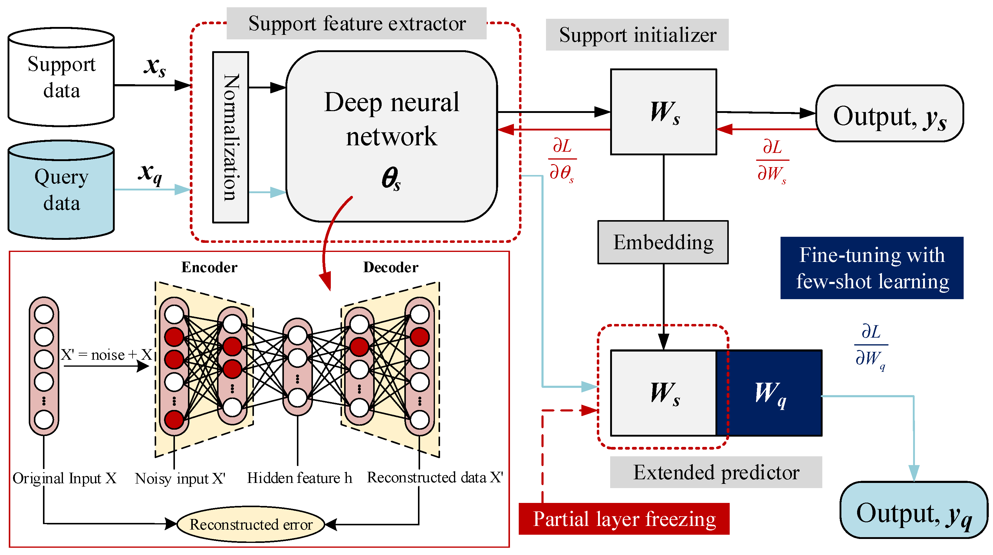
Therefore, this study proposes a model development framework using LSTM with simulation-assisted few-short learning (FSL-LSTM) for predicting and optimizing the glycerin product purity of the glycerin purification process and water removal of the evaporating unit under feed uncertainty and limited data. The model is trained to create a support feature extractor and weight initializer using a simulated support set, which is then used to fine-tune the prediction model in the limited data domain using a query set obtained from the large-scale glycerin purification unit. The main contribution of the proposed procedure is summarized as follows:

• Develop a glycerin purification process simulation model to determine optimal operating conditions and generate data for the support set.
• Formulate a robust predictive model based on deep learning constructed using LSTM structure fine-tuning based on few-shot learning techniques for tracking the refined glycerin production capacity and water content of refined glycerin under multiple operating conditions.
• Reveal the relationship between the input variables and the target variables of the prediction model to enhance the production capacity and water content using the proposed model.

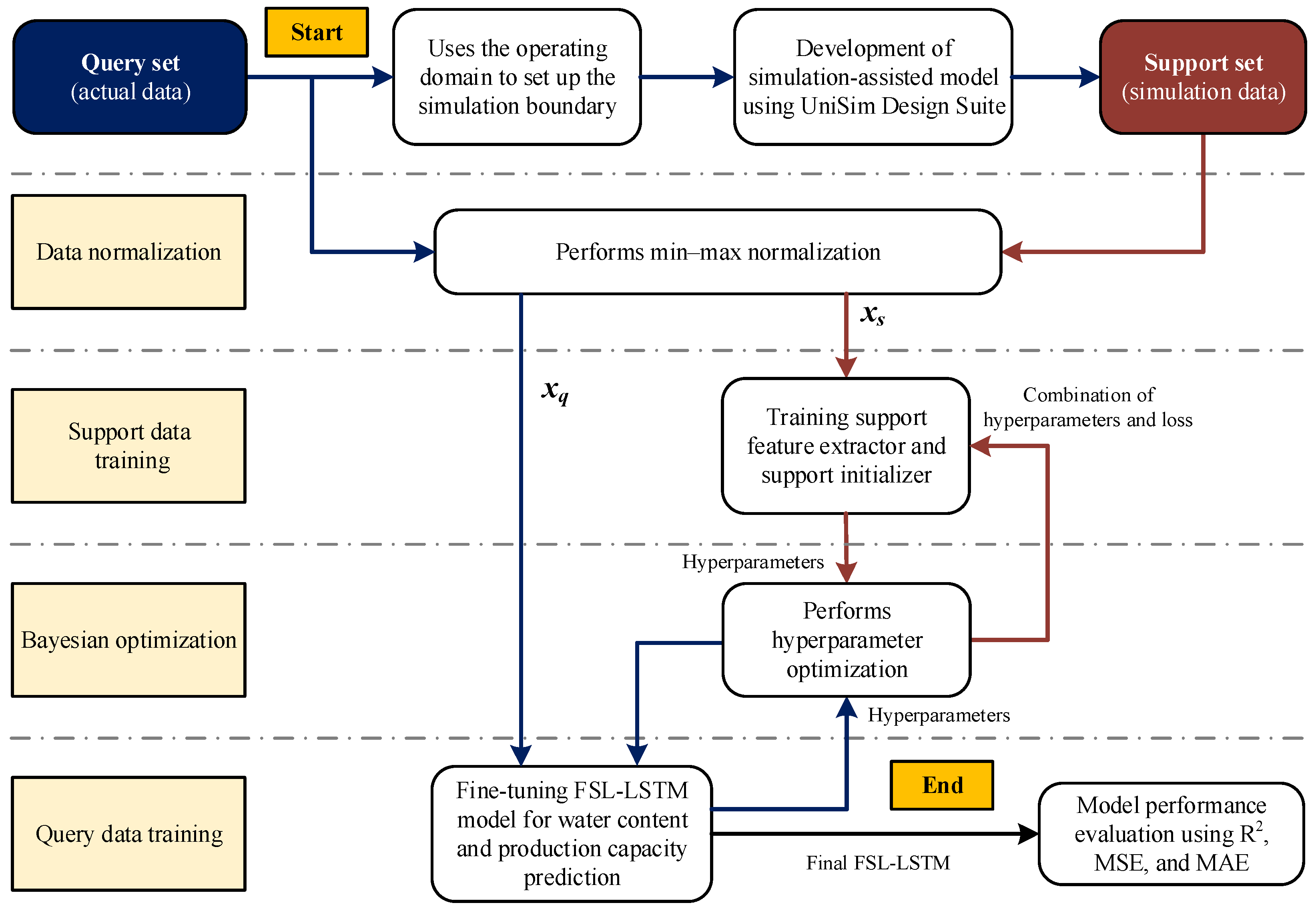
The remainder of this work is divided into the following sections: Section 2 explains the concept of modeling procedures in developing FLS-LSTM, which includes few-shot learning, LSTM architecture, and Bayesian optimization. Section 3 presents the case study utilized in this study, incorporating a system description and comparative analysis of support and query data. Section 4 shows the performance of the proposed model in predicting glycerin production and water content, the accuracy–iteration tradeoff, and the production optimization results. Finally, conclusions are drawn in Section 5.

2. Materials and Methods

2.1. Simulation-Assisted Few-Shot Learning

Few-shot learning stands as a technique enabling models to understand or infer information from a very limited amount of data [27], which is the main focus of this study. Figure 2 depicts the schematic of a simulation-assisted few-shot learning system designed to enhance the learning process by integrating simulated support data. The system comprises several key components:

• Support and query data: The model operates on two datasets, including the support data (x_s), which are excess data used to pre-train the model obtained by simulation, and the query data (x_q), which refer to the limited data used to fine-tune and evaluate the model’s generalization using actual data from the large-scale glycerin purification process.
• Deep neural network: A deep neural network, in this case, variational autoencoder (VAE), functions as a feature extractor. The VAE typically consists of two parts: an encoder that reduces the input data to a lower-dimensional space and a decoder that attempts to reconstruct the input data from this latent space [28]. The loss function of VAE can be split into two components. The first component is the reconstruction loss ($L_{rec}$). For a given datapoint $X_i$, the reconstruction loss is computed as the mean squared difference between $X_i$ and its reconstructed counterpart (${\widehat{X}}_i$), formulated as Equation (1). The particular component provides an incentive for the reconstructed output to closely replicate the original input.

  $$L_{rec}({\theta }_s,x_i)={‖X_i-{\widehat{X}}_i‖}^2$$

  (1)

  Next, the Kullback–Leibler divergence ($L_{KL}$) is calculated as Equation (2), quantifying the discrepancy between the approximate posterior distribution and the assumed prior distribution [29]. The encoder is tasked with outputting the means ($\mu$) and the logarithm of the variance ($\sigma$) of the latent dimensions, ensuring numerical stability.

  $$L_{KL}({\varphi }_s,X_i)=\frac{1}{2}{\displaystyle {\sum }_{j=1}^J({\sigma }_j{(X)}^2+{\mu }_j{(X)}^2-1-\log {\sigma }_j{(X)}^2)}$$

  (2)

  Through the aggregation of these losses across the datapoints within the dataset, the overall loss function can be calculated as Equation (3).

  $$L_{vae}({\theta }_s,{\varphi }_s;X)=\frac{1}{N}{\displaystyle {\sum }_{i=1}^N(L_{rec}({\theta }_s,X_i)+L_{KL}({\varphi }_s,X_i)})$$

  (3)

  where ${\theta }_s$ and ${\varphi }_s$ refer to the learnable parameters of the decoder and encoder networks, respectively.
• Normalization block: Within the neural network, a normalization procedure is applied to regulate the feature scaling. This can significantly help the model maintain and stabilize the training dynamics. Both input and output variables are rescaled into zero to one (a = 0, b = 1) using Equation (4).

  $$X_{rescaled}=a+\left[\frac{X-{\min }_x}{{\max }_x-{\min }_x}\right](b-a)$$

  (4)
• Support initializer and extender predictor: The initializer is used to create the initial predictor weights (W_s) based on the support data, embedding the gained knowledge into the model. This part of the model was constructed using the LSTM layer (discussed in Section 2.2) for both domains. Subsequently, the extended predictor undergoes a few-shot learning phase using the limited query data to predict the final output (y_q). In this step, partial layer freezing is applied to the initial weights to prevent overfitting and preserve previous knowledge gained from the support data while adapting to the specific query data. Only the modifying weights (W_q) are adjusted during fine-tuning using the loss gradient from the query data, where the loss is a half-mean-squared error (HMSE) calculated by Equation (5). The local learning rate of the initial weight is set to zero during the fine-tuning step.

  $$L_{HMSE}=\frac{1}{2N}{\displaystyle \sum _{i=1}^M{(y_i-{\widehat{y}}_i)}^2}$$

  (5)

  where $y_i$ is the prediction value, ${\widehat{y}}_i$ is the target value, M is the total number of responses in $y_i$, and N is the total number of observations in $y_i$. The learnable parameters of FSL-LSTM are updated using adaptive moment estimation (ADAM) algorithms [30], as shown in Equation (6).

  $$w_{t+1}=w_t-{\eta }_g{\eta }_l\frac{{\widehat{m}}_t}{\sqrt{{\widehat{v}}_t}+\epsilon }$$

  (6)

  where ${\eta }_g$ and ${\eta }_I$ are the global (hyperparameter of the model) and local learning rates of the model, $\epsilon$ is a small constant for numerical stability, and ${\widehat{m}}_t$ and ${\widehat{v}}_t$ are the bias-corrected estimates of the first and second moments calculated by Equations (7) and (8).

  $${\widehat{m}}_t=\frac{{\beta }_1\cdot m_{t-1}+(1-{\beta }_1)\cdot {\nabla }_{w}L}{(1-{\beta }_1)}$$

  (7)

  $${\widehat{v}}_t=\frac{{\beta }_2\cdot v_{t-1}+(1-{\beta }_2)\cdot {({\nabla }_{w}L)}^2}{(1-{\beta }_2)}$$

  (8)

  Finally, the gradient of the loss function with respect to the model parameters for the fine-tuning step is calculated using Equation (9). The use of the local learning rate as a binary switch in this context controls whether the specific parameters within the network are updated or not during the fine-tuning phase [31]. When the weight vector is the learnable parameter related to the support initializer and the local learning rate is 0, it implies that the gradients do not contribute to the weight update, effectively enabling selective training where certain parts of the model are kept static to retain pre-trained knowledge [32]. In contrast, for the extended predictor, local learning equal to 1 signifies that the weights are actively being fine-tuned.

  $${\nabla }_{w}L=\frac{\partial L}{\partial w}\left\{\begin{array}{c}w=w_s,{\eta }_l=0\\ w=w_q,{\eta }_l=1\end{array}\right.$$

  (9)

The proposed framework begins with using the information from the query set to set up the simulation boundary. This is followed by the development of the simulation-assisted model using the UniSim Design Suite to generate a support set (simulation data). The process continues with data normalization performed on both domains. Next, the model uses the information from x_s to train the support feature extractor and initializer, preparing the model with initial parameters that can be further refined. Bayesian optimization is applied in this step to find the best combination of hyperparameters such as the hidden node, learning rate, and regularization factor.

Once the support data training is completed and the optimal hyperparameters for the support set are identified, the fine-tuning of the FSL-LSTM model using x_q is performed. Again, Bayesian optimization is applied to find the hyperparameters for the query set. Finally, the process concludes with the final FSL-LSTM model, which is then evaluated for its performance using metrics such as the coefficient of determination (R²), mean squared error (MSE), and mean absolute error (MAE), calculated by Equations (10)–(12), respectively. These metrics provide a quantitative measure of how well the model is performing, indicating its accuracy and precision in predicting glycerin production and water content based on the limited query data. The overall framework for developing the FSL-LSTM framework is summarized in Figure 3.

$$\mathrm{MSE}=\frac{1}{n}{\displaystyle \sum _{i=1}^n{(y_i-{\stackrel{⌢}{y}}_i)}^2}$$

(10)

$$\mathrm{MAE}=\frac{1}{n}{\displaystyle \sum _{i=1}^n\left|y_i-{\stackrel{⌢}{y}}_i\right|}$$

(11)

$${\mathrm{R}}^2=1-\frac{{\displaystyle {\sum }_i{(y_i-\widehat{y})}^2}}{{\displaystyle {\sum }_i{(y_i-\overline{y})}^2}}$$

(12)

In summary, each step in the framework of FSL-LSTM plays a vital role in ensuring that the model is not only pre-trained on a broad range of simulated data but also finely tuned to real-world scenarios. This modeling approach allows for a more robust and adaptable model capable of handling complexities and limited data problems without raising concerns about domain differences.

2.2. LSTM Network Architecture

Handling complex relationships, such as the information from industrial processes, requires a network that can capture temporal dynamics and long-term dependency [28]. In recent years, LSTM has emerged as a fundamental component in the field of deep learning, especially for tasks that require processing sequential and time-series data. An LSTM network consists of a sequence of recurrent modules called LSTM cells. Every cell comes with gates, which are systems that control the flow of information inside the LSTM structure. These gates—the forget gate, input gate, and output gate—allow LSTMs to selectively remember and forget patterns over long sequences of data, as visualized in Figure 4. Inside the LSTM layer, the long-term memory is updated at the forget gate using the cell state of the previous timestep using Equation (13).

$$f_t=sigmoid(W_{xf}{X}_t+W_{cf}{h}_{t-1}+b_f)$$

(13)

Then, the input gate filters out unnecessary information, and only a significant part of the input will perform point-wise multiplication with the old state variable to create a cell candidate using Equations (14)–(16).

$$i_t=sigmoid(W_{xi}{X}_t+W_{ci}{h}_{t-1}+b_i)$$

(14)

$$g_t=tanh(W_C{X}_t+W_C{h}_{t-1}+b_c)$$

(15)

$$C_t=C_{t-1}\times f_t+i_t\times g_t$$

(16)

At the output gate, the updated cell state is used to determine the final values of the hidden state for the next layers using Equations (17) and (18).

$$o_t=sigmoid(W_{XO}{X}_t+W_{CO}{h}_{t-1}+b_o)$$

(17)

$$h_t=o_t\times tanh(C_t)$$

(18)

A state $C_t$ contains a unit of LSTM at the time $t$, and it is controlled through the forget gate $f_t$, input gate $i_t$, candidate cell $g_t$, and output gate $o_t$; $x_t$ is the vector of input variables at the time $t$, and $h_{t-1}$ is the previous value of the hidden state.

2.3. Bayesian Optimization for Hyperparameter Tuning

Bayesian optimization acts as a strategic tool in this process, seeking to fine-tune the hyperparameters by iteratively minimizing the objective function, which is used in this study for validating the MSE. Figure 5 illustrates the utilization of Bayesian optimization for tuning the hyperparameters in a glycerine purification process model. The process begins with the training model acting as an observer to evaluate the initial combination of hyperparameters for fitting the surrogate model (Gaussian process regression). The expected improvement (EI) acquisition function, calculated using Equation (19), then guides the selection of subsequent hyperparameters, aiming to maximize the expected improvement over the best current validation MSE. This is particularly useful in a few-shot learning scenario, where the model needs to generalize well from a limited amount of data. By carefully choosing where to sample next, EI helps to efficiently navigate the hyperparameter space specified in

Table 2. The search domain for hyperparameter tuning using Bayesian optimization.

Hyperparameters	Value
Number of FNN hidden layers	[1–100]
Number of LSTM hidden node	[1–5]
Number of LSTM hidden layers	[1–100]
Number of LSTM hidden node	[1–5]
Number of NARX hidden layers	[1–100]
Delay of NARX network	[1–5]
Number of RNN hidden layers	[1–100]
Delay of RNN network	[1–5]
Initial learning rate	[1 × 10−1–1 × 10−5]
L2 Regularization	[1 × 10−1–1 × 10−4]
Max training iteration	500
Optimizer	[ADAM, RMSProp, SDG]

, reducing the number of iterations needed to find an optimal set of hyperparameters compared to optimization techniques such as grid search. The process is performed iteratively until the specified iteration is reached (50 iterations), indicating that the model has potentially reached an optimum. The outcome of this process is a set of hyperparameters finely tuned to the few-shot learning task, which will be used as a final model for glycerine production and water content optimization.

$$EI(x,Q)=E_Q[\max (0,{\mu }_Q(x_{best})-f(x))]$$

(19)

where $x_{best}$ is the location of the lowest posterior mean and ${\mu }_Q\left(x_{best}\right)$ is the lowest value of the posterior mean.

3. Glycerin Purification Case Study

3.1. Process Description

Figure 6 illustrates the process flow diagram of the glycerin purification process under study. The process comprises three main units: neutralization, evaporation, and glycerin distillation. Initially, the crude glycerine feed, containing glycerin, water, fatty acids, and other impurities, is preheated in a heat exchanger. This pre-treatment step is crucial before sending the mixture to the neutralization unit. In the neutralization unit, a sodium hydroxide solution (at a ratio of 0.5 mol/mol and room temperature) is used to adjust the pH to a range of 7.0 to 9.0.

Since the water content significantly affects the purity of glycerin during production, the neutralized mixture is then forwarded to the evaporation unit. Here, the mixture undergoes drying through a water evaporation process. Since water has a much lower boiling point than glycerin, this step effectively reduces the water content. The evaporator’s temperature must be carefully adjusted according to the feed compositions to achieve the desired water content, making evaporation a critical stage in the process. The target is to reduce the water content of the mixture to below 2% before proceeding to the next stage. Subsequently, the glycerin, now with reduced water content, is sent to a distillation column for further purification. The distillation process aims to achieve a glycerin purity of 98–99%. The column used for this purpose is a five-stage structurally packed column equipped with a two-stage rectifier and a total condenser. The primary role of each unit operation included in glycerin purification is given in

Table 3. Role of each simulation unit operation in the glycerin purification process.

Operation	Equipment	Unit	Duty
Neuralization process	Gibbs reactor	S-100	A vessel that occurs in a transesterification reaction to obtain an outlet glycerin stream.
Evaporation process	Heater	H-101	Heat the mixed glycerin stream to 120 °C
	Evaporator 1	S-101	Evaporate vapor stream and liquid glycerin stream
	Cooling	C-100	Condense glycerin in the vapor stream
	Evaporator 2	S-102	Evaporate condensed glycerin and vapor of impurity
	Pump	P-101	Boost pressure
Purification process	Distillation column	D-100	Purify glycerin to the desired purity
	Condenser	C-101	Condense an alloy glycerin to distillate
	Reboiler	H-103	Heat glycerin returns to distillation and to the bottom product

.

In this study on glycerin purification, a series of input variables are identified to influence the output characteristics of the process. The glycerin and water content in the feed (X1 and X2) directly affect the quality of the output, as they determine the starting composition of the purification process. The mass flow rate of the feed (X3) and the distillation column feed rate (X5) are crucial for the throughput of the system, influencing both the production capacity (Y1) and the efficiency of the water removal (Y2). The inlet temperature of the first heat exchanger (S-101) and the bottom temperature of the distillation column (X6) are key thermal inputs that drive the separation process, while the top and bottom pressures of the distillation column (X7 and X9) and the top temperature of the side stream (X10) are indicative of the energy and material balances within the system. The relationship between these inputs and the outputs—namely, the production capacity and the remaining water content in the purified glycerin—illustrates the complex interplay of thermal and material transfer within the purification process, where the list of input and output variables used in this study is given in

Table 4. List of input and output variables used in this study.

No.	Variable Name	No.	Variable Name
X1	Glycerin content in feed, wt.%	X7	D-100 bottom pressure, bar
X2	Water content in a feed, wt.%	X8	D-100 top temperature, °C
X3	Feed mass flow rate, kg/h	X9	D-100 top pressure, bar
X4	S-101 inlet temperature, °C	X10	Top temperature of side steam D-100, °C
X5	Distillation column feed rate, kg/h	Y1	Remaining water at evaporator outlet, wt.%
X6	D-100 bottom temperature, °C	Y2	Production capacity, kg/h

.

3.2. Process Simulation Modeling

The simulation of the glycerin purification process was developed in the UniSim Design Suite R460.1 software using the nonrandom two-liquid thermodynamic and fluid model. To create comprehensive datasets, we utilized a co-simulation environment, integrating MATLAB R2023b with the UniSim Design Suite process simulator. This approach enabled us to simulate various process conditions, generating a substantial amount of data with 1000 sample points. Such a method ensures that our simulated data (support data) adequately represent the actual operational conditions (query data).

To verify that the data obtained from digital twins can represent the real system, this study carried out the Wilcoxon rank sum test [33]. The heatmaps provided in Figure 7a,b offer a comprehensive visual assessment of the Wilcoxon rank sum test results applied to the virtual data generated by the digital twins. The p-values shown in Figure 7a, which are uniformly above the 0.05 significance threshold at 1000 generated samples, suggest that the differences observed in the median values of the digital twin data and the real system data across 1000 samples are not statistically significant. The rank sum test compares the median of the two samples by considering the ranks of all observations. A higher p-value implies that the probability of observing the data under the null hypothesis (the hypothesis that there is no difference between the distributions) is high. Consistently accepted hypotheses in Figure 7b, indicated by zeros (null hypothesis), reinforce the p-value findings. This binary heatmap indicates that for every instance, the null hypothesis posits that the data from the digital twin and the real system are from the same distribution. The alignment between high p-values and the acceptance of the null hypothesis across all tested instances provides robust evidence that the digital twin is capable of producing data that statistically reflects the real behavior of the system.

During the simulation, the crude glycerin feed compositions varied. The adjustments included a range of 10–20% water content, 80–90% glycerin content, 1–2% Matter Organic Non-Glycerol (MONG) content, and an acidity content between 0.06 and 0.1%. Additionally, the feed rate of the crude glycerin was altered between 3700 kg/h and 4500 kg/h. To replicate varying operational conditions, the top temperature of the distillation column, operating at atmospheric pressure, was modified between 120 °C and 125 °C. The simulation domain is summarized in

Table 5. The parameter range on the glycerin purification process.

Name of Variable	Units	Setpoint	Range
Feed crude glycerin
Feed mass flow rate	kg/h	3000	[2500–4000]
Component
Glycerin	wt.%	88	[80–90]
Water	wt.%	10	[10–20]
Evaporator
Inlet temperature	°C	120	[120–134]
Distillation column
Feed rate	kg/h	2700	[2300–3000]
Top temperature	°C	125	[125–130]
Top pressure	bar	0.0025	[0.001–0.005]
Bottom temperature	°C	160	[155–165]
Bottom temperature	bar	0.0045	[0.002–0.007]
Return top temperature	°C	134	[130–137]

.

Upon obtaining the 1000 data samples, the whole dataset was partitioned into distinct sets for training, validation, and testing. The distribution was as follows: 80% for training, 10% for validation, and the remaining 10% for the test set. The 80% in the training set was used to train the model, while the 10% in the validation set was used to evaluate the objective performance during hyperparameter optimization. Finally, the last 10% of the testing dataset was applied to assess the performance of the final model after finishing the training and hyperparameter tuning.

The histograms in Figure 8 display a comparison of simulated and actual operational data, providing insight into the potential to broaden the operating range of the process. Areas of strong overlap between support and query data indicate close alignment, suggesting the simulation reflects the validated operational range accurately, suggesting a high degree of correlation between the simulated environment and real-world operations. The proximity of the mean values across various parameters implies that the simulation can effectively mirror the actual process, making it a valuable tool for exploring extensions to the operating domain. Densities in the histograms suggest the frequency of certain conditions in both sets of data; when simulation data are denser at the extremes, it may indicate the potential for stable operation beyond currently observed limits.

4. Result and Discussion

4.1. Water Content and Production Capacity Prediction Result

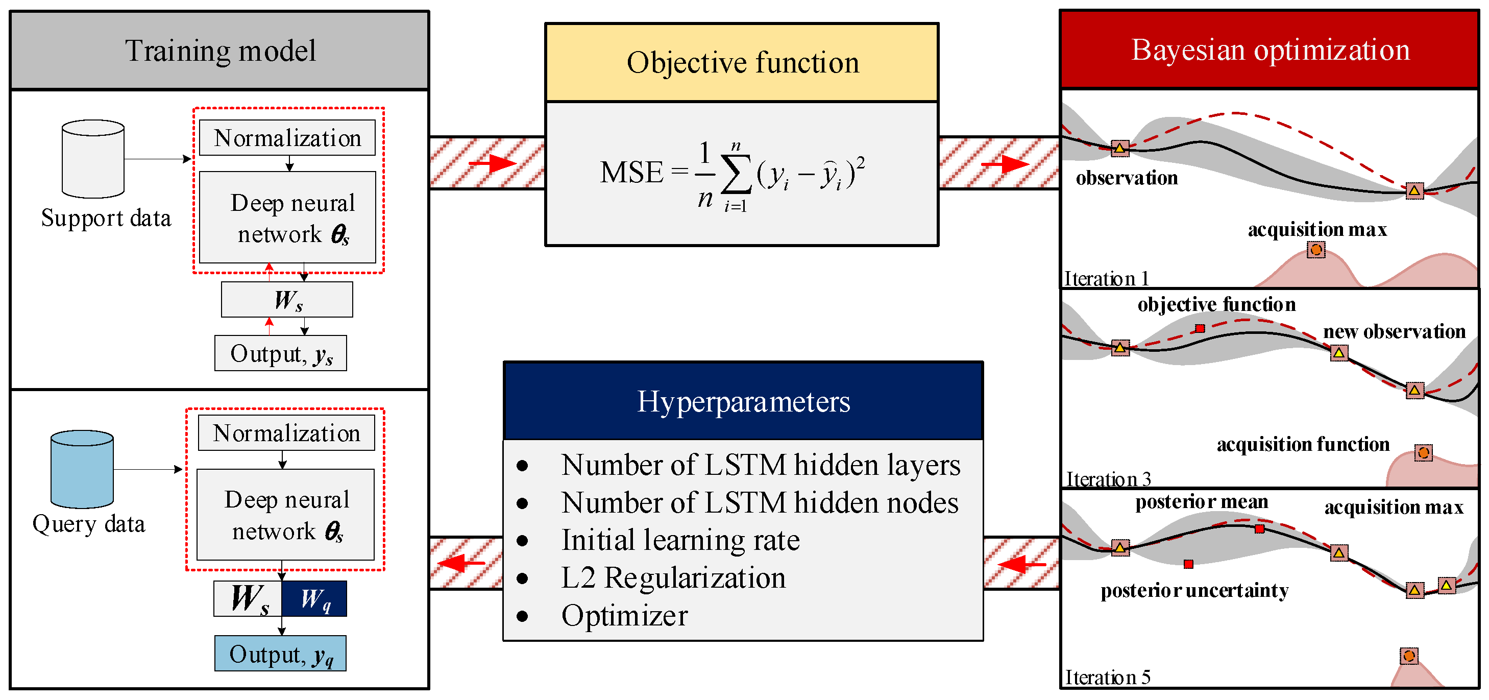
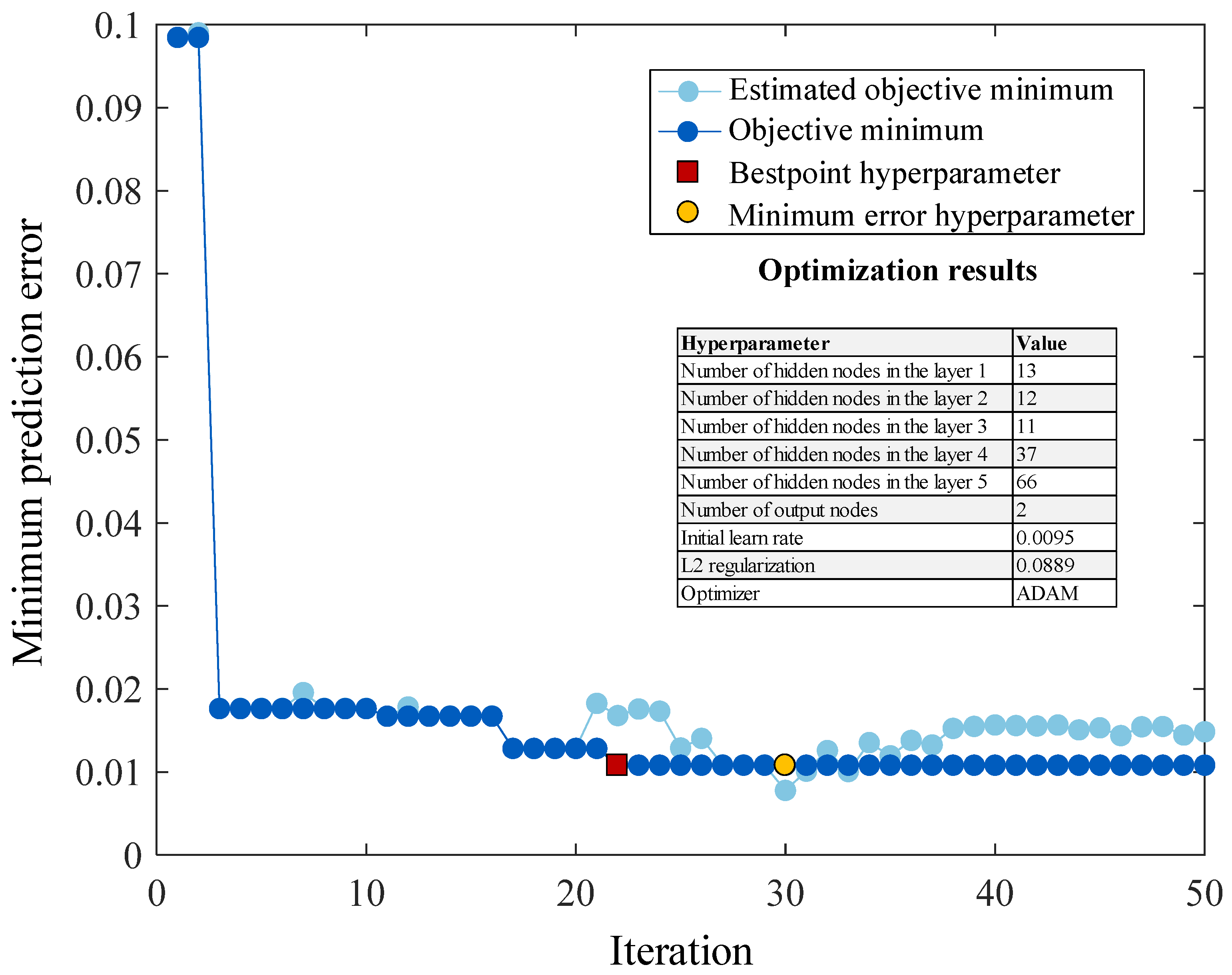
The hyperparameter optimization applied to the FSL-LSTM using nine selected hyperparameters is shown in Figure 9. These optimized hyperparameters, chosen for observation, include the number of hidden layers, the number of hidden nodes, the initial learning rate, the L2 regularization, and the optimizer. As the number of iterations increases, the prediction error steadily decreases. This ongoing reduction indicates that the optimization process is effectively identifying better hyperparameter combinations. Notably, the FSL-LSTM model, after hyperparameter optimization, exhibits a significant decrease in the minimum prediction error. This error drops from 0.1 to 0.02 as early as iteration 2 and remains stable until reaching its lowest point, 0.0149, at iteration 22. This minimum error value lies close to the estimated objective minimum line, further validating the effectiveness of the optimization approach. The best set of hyperparameters is located at 22 iterations. One essential point is that the optimal value for the learning rate is 0.0095. Furthermore, the remarkably low learning rate of 0.0095 highlights the importance of carefully adjusting the model’s pre-trained knowledge during fine-tuning. This minimal step size helps safeguard the valuable information encoded in the initial model, allowing it to serve as a strong foundation for learning task-specific details without causing a catastrophic forgetting of its general capabilities. This reflects that the pre-trained knowledge gained from the support data significantly helps the model during the training phase.

The comparative results of water content prediction focusing on the testing performance of the model are presented in

Table 6. The performance evaluation results of water content prediction using a testing set.

Method	MSE	MAE	R2
FNN	0.009	0.038	0.793
RNN	0.067	0.099	0.204
NARX	0.075	0.105	0.149
LSTM	0.009	0.043	0.801
AM-LSTM	0.004	0.051	0.918
MC-LSTM	0.004	0.037	0.849
FSL-LSTM	0.001	0.017	0.995

: the performance accuracy of the testing model of water content. The FSL-LSTM model demonstrates a notable R² value of 0.995, thereby evidencing its superior predictive accuracy compared to other traditional models: 0.793 for FNN, 0.204 for RNN, 0.149 for NARX, and 0.801 for LSTM. The result demonstrates that the FSL-LSTM provided a 24.2% improvement in R² values in the case of the LSTM with custom few-shot learning. When comparing the performance of advanced LSTM models, the AM-LSTM and MC-LSTM also show substantial predictive accuracy, with R² values of 0.918 and 0.849, respectively. The FSL-LSTM, however, surpasses the AM-LSTM with an R² value improvement of 8.3%, underscoring the significant impact of the few-shot learning approach in refining predictive performance. The FSL-LSTM model, which employs a digital twin to generate data, shows a 17.2% improvement in R² value over the MC-LSTM. This suggests that the synthetic data generated from the digital twin, when combined with real-world fine-tuning, result in a model that is not only robust but also highly precise in its predictions.

The effectiveness of the proposed model is further revealed by MAE values of 0.017, thereby surpassing the MAE values of FNN, RNN, NARX, LSTM, AM-LSTM, and MC-LSTM, which have MAE values of 0.038, 0.099, 0.105, 0.043, 0.0051, and 0.037, respectively. In comparison to traditional LSTM, incorporating few-shot learning fine-tuning with a simulation-assisted model reduced errors by 60% up to 83% when compared to other models in the study. Additionally, in the case of MSE values, the FSL-LSTM model records a minimal MSE value of 0.001, markedly lower than those recorded by FNN (0.009), RNN (0.067), NARX (0.075), LSTM (0.009), AM-LSTM (0.004), and MC-LSTM (0.004) with an error reduction of up to 98%.

Table 7. The performance evaluation result of glycerin production prediction using a testing set.

Method	MSE	MAE	R2
FNN	0.011	0.054	0.541
RNN	0.028	0.056	0.309
NARX	0.036	0.055	0.397
LSTM	0.012	0.057	0.498
AM-LSTM	0.025	0.138	0.562
MC-LSTM	0.009	0.052	0.572
FSL-LSTM	0.006	0.050	0.895

shows the comparative analysis for the glycerin production prediction using a testing dataset of glycerin production predictions. The FSL-LSTM model attains an R² value of 0.895, outstripping FNN (0.541), RNN (0.309), NARX (0.397), LSTM (0.498), AM-LSTM (0.562), and MC-LSTM (0.572), which is a 79.7% improvement in R² values compared to the traditional LSTM. Additionally, the R² performance improvement for the glycerine production prediction is higher than the improvement in water content.

In evaluating the MAE loss variable within this context, the FSL-LSTM model records an MAE of 0.050, a value that is demonstrably lower than those recorded by FNN (0.054), RNN (0.056), NARX (0.055), LSTM (0.057), AM-LSTM (0.138), and MC-LSTM (0.052). Despite the marginal disparities among the training models, the FSL-LSTM model exhibits a significantly reduced MAE value, exhibiting a 12.2% error reduction. Conclusively, the MSE evaluation of the model for production capacity further corroborates the superiority of the FSL-LSTM model. With an MSE value of 0.006, it presents a notable error reduction of 50% compared to the LSTM model.

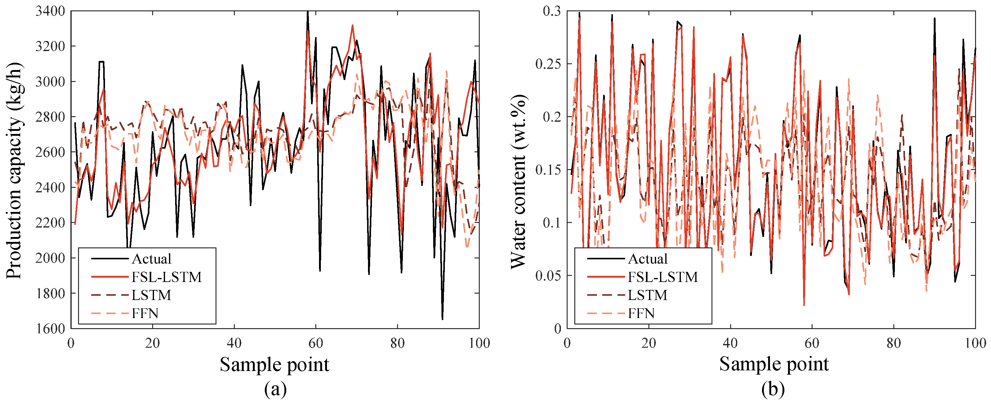
Figure 10a shows the predicted glycerin production capacity values from three different training models: the LSTM model, the FNN model, and the FSL-LSTM model, compared with the actual values (represented by a black line). Among these, the FSL-LSTM model (indicated by a red line) most accurately simulates changes in production capacity, closely aligning with the actual values. In contrast, the predictions from the LSTM model (shown in dark red) and the FNN model (depicted in orange) are less accurate, as evidenced by the divergence of their respective lines from the actual values, where the FSL-LSTM can track the abrupt process transition in changing production capacity.

Figure 10b focuses on the prediction performance of water content using FSL-LSTM. Here, the FSL-LSTM model is again notable for its accuracy, with its predictions (red line) closely mirroring the actual values. The LSTM model, while capable of capturing some characteristics of the actual data, falls short of the performance demonstrated by the FSL-LSTM model. Even in the water content prediction, where the noise in the process is relatively larger than the glycerin production prediction, the FSL-LSTM can accurately predict the water content under this scenario.

4.2. Domain-Specific Testing Result Using Unseen Data

Table 8. Robustness testing result of FSL-LSTM on extended data beyond training domain.

Output	Type	MSE	MAE	R2
Water content	Simulated	0.0004	0.012	0.992
	Actual	0.005	0.033	0.910
Glycerin production	Simulated	0.0003	0.007	0.994
	Actual	0.014	0.069	0.790

provides an overview of the robustness of the FSL-LSTM model when assessing its performance on data that extends beyond the training domain. The ‘simulated’ category denotes scenarios that have never been operated before in real operational data. In this case, the model exhibits an outstanding predictive accuracy for water content, with an R² of 0.992 and a minimal MSE of 0.0004. For glycerin production under the same conditions, the predictive strength of the proposed model is further underscored by an even higher R² of 0.994 and a low MSE value of 0.0003.

When the ‘actual’ operational data, which are not fundamental simulation knowledge from the digital twin and lie outside the training domain, are considered, the performance of FSL-LSTM is slightly decreased in the water content prediction task. The impact is more pronounced in the case of glycerin production prediction, where the R² value decreases to 0.790. This reduction is not extreme when considering the high benchmark set by the model in normal testing scenarios, where an R² of 0.895 was achieved. The decrease in R² can be attributed to the model grappling with unique operational scenarios presented by the actual data that extend beyond its trained and simulated experience. Despite this, it is important to note that the performance of the FSL-LSTM model, even with these limitations, remains higher than other methods evaluated under normal testing conditions. This suggests that while the reduction in performance is discernible, it is relatively slight, and the model maintains a degree of predictive resilience that surpasses conventional approaches.

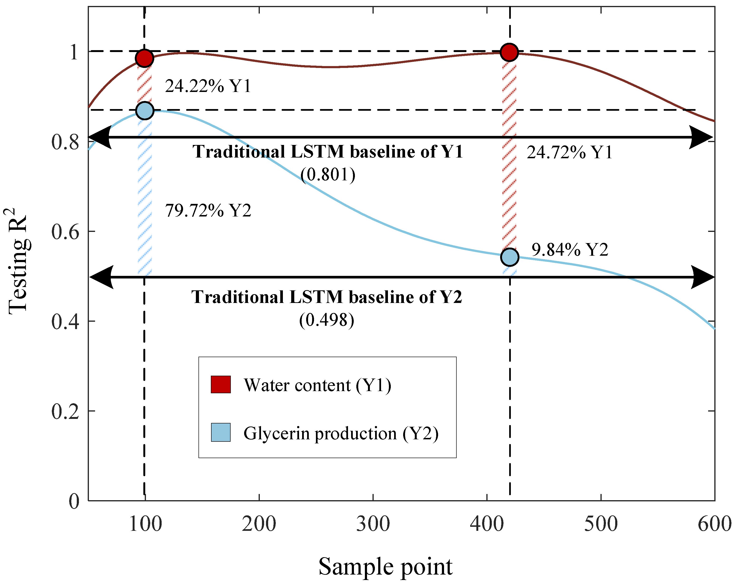
4.3. Accuracy–Iteration Tradeoff in Few-Shot Learning LSTM

Figure 11 shows the result of decreasing and increasing the number of iterations in few-shot learning techniques. The model selection of FSL-LSTM is determined by the tradeoff between accuracy improvement among two outputs. The best number of iterations is obtained at two locations on this plot, 100 (maximum testing R² of glycerin production is located) and 440 iterations (maximum testing R² of water content is located). At 100 iterations, the testing R² values of Y1 and Y2 are 0.995 and 0.895, respectively, while the traditional LSTM performances without fine-tuning using few-shot learning are 0.801 for Y1 and 0.498 for Y2. The decision on accuracy–iteration in few-shot learning is determined by the percentage of relative improvement (RI), which is calculated using Equation (20).

$$\mathrm{RI}=\left[\frac{B_{FSL-LSTM}-B_{LSTM}}{B_{LSTM}}\right]\times 100\%$$

(20)

Denoted by the $B_{FSL-LSTM}$ is the testing R² value of Y1 or Y2 from the few-shot learning, and $B_{LSTM}$ is the testing R² value of Y1 or Y2 from the traditional LSTM baseline. Calculating the RI value is an essential step in assessing the performance gains achieved by the FSL-LSTM model over the traditional LSTM baseline, which provides a quantifiable measure of improvement in predictive accuracy.

At maximum testing R² of glycerin production, this point provided a 24.22% improvement in water content prediction and a 79.72% improvement in glycerin production over the LSTM baseline. Furthermore, at 440 iterations, the R² value of testing data for Y1 is 0.999, while for Y2 it is 0.547. At this point, the few-shot learning significantly improved the performance in water content prediction by up to 24.72%. However, the large improvement in Y2 results in an overfitting problem in Y1, where the testing performance drops substantially with only a 9.84% improvement. Thus, the justification of iteration count should be made with a primary focus on glycerin production prediction performance, and in this context, 100 iterations (one datapoint per iteration) prove to be the optimal selection for few-shot learning with FSL-LSTM.

4.4. Production Optimization Results

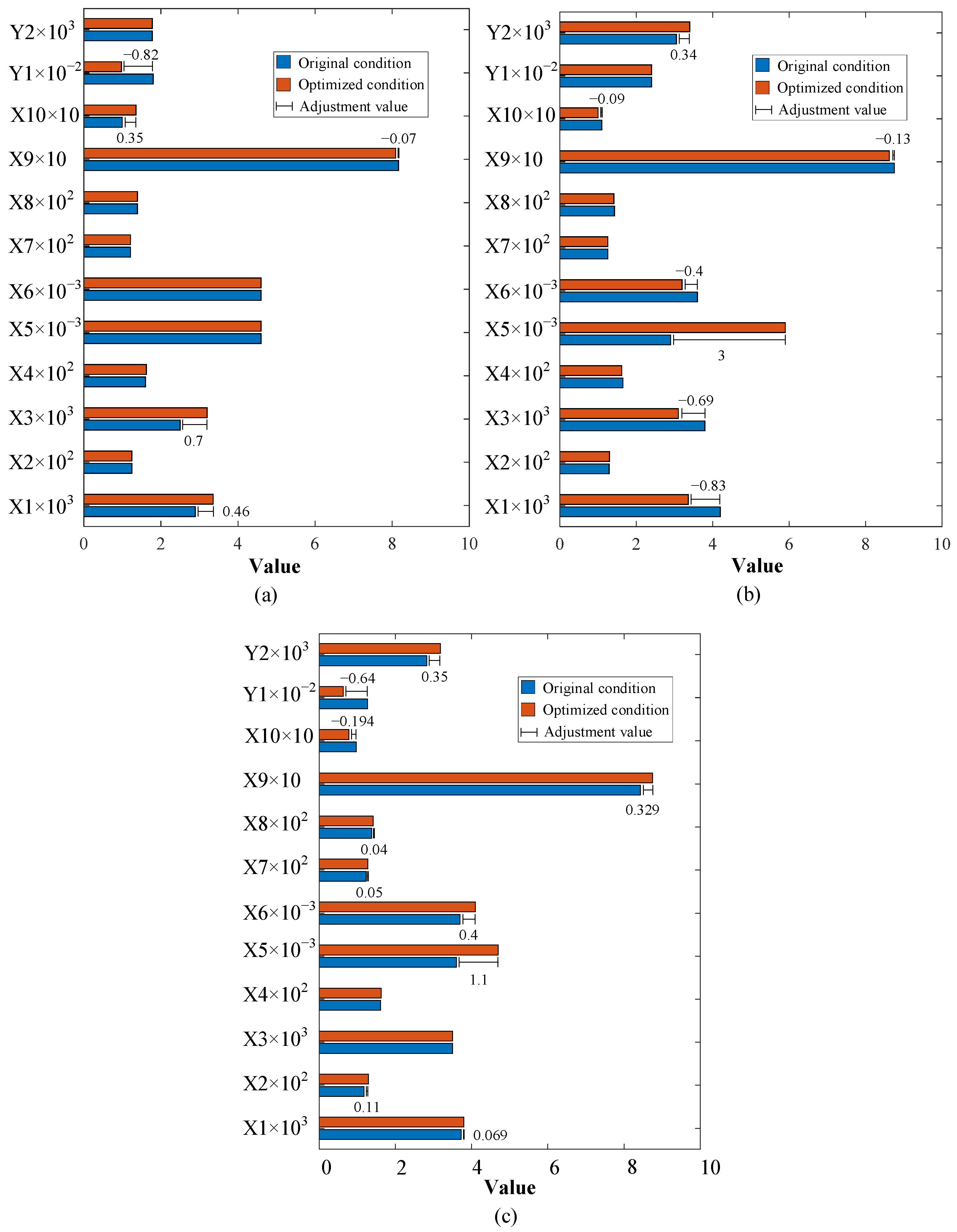
After the FSL-LSTM is finally tested for its ability to track water content and glycerin production, an operating condition adjustment is performed on the model to find the optimal condition for the glycerine purification process based on the prediction sensitivity. For example, Figure 12a shows the operational adjustment result for optimizing water content without changing glycerine production capacity. It can be seen that if X1 and X3 are increased by 0.46 and 0.7 while X9 is reduced by 0.07, the water content of the final glycerin product can be reduced by 0.35. The system manipulation of the feed composition and operational pressure enhances the separation efficiency, minimizing the need for excessive heat and mitigating the thermal stress on the distillation equipment. Operating the column under conditions that avoid extremes in temperature and pressure variations fosters process stability, lowering the risk of overpressure incidents.

In Figure 12b, there are optimization results for production maximization while the final water content remains constant. This can be performed by reducing X1, X3, X6, X9, and X10 by 0.83, 0.69, 0.4, 0.23, and 0.09, respectively, and increasing X5 by 3. The production of glycerin will be improved by 0.34. The significant gap in X5 indicates a potential underutilization of the existing distillation unit due to unused capacity within the column internals. Overall, these results illustrate the effectiveness of the FSL-LSTM model in guiding targeted operational adjustments for the glycerin purification process under limited operating data and working domains. Lowering the bottom temperature of the column implies that the energy supplied to vaporize the feed is minimized, which can both reduce the thermal degradation of heat-sensitive components such as glycerin and decrease the energy consumption of the separation process.

In aiming to optimize both glycerin production and water content, an increase in the distillation column feed rate and adjustments in temperature at strategic points of the process highlight the ability to enhance both productivity and product purity, as shown in Figure 12c. However, adjusting X1 and X3 has counteracting effects on Y1 and Y2. Increasing X1 and X3 actually leads to a reduction in Y1, as a richer glycerin feed and increased feed mass flow effectively decrease the remaining water content in the final product. Conversely, reducing X1 and X3 can lead to an increase in Y2, facilitating a more manageable load on the distillation system. Considering these counteracting effects, other operational variables become a strategic approach. According to Figure 12c, increasing X5 (by 1.1), X6 (by 0.4), and X9 (by 0.329) while reducing X10 (by 0.194) offers a path to optimize the distillation conditions for both separation efficiency (by 0.64) and production capacity (by 0.35). By boosting X5, the throughput of the distillation column is increased, directly contributing to a higher production capacity, while the precise increase in X6 and X9 enhances the vaporization dynamics and condensation dynamics, improving the separation of glycerine from water. Simultaneously, the reduction in X10 aims to optimize energy efficiency and further refine the separation process by carefully managing the thermal conditions. The adjustment ensures that the process not only meets its production goal but also improves product purity, illustrating a sophisticated balance between process efficiency, energy consumption, and product quality in the face of complex operational tradeoffs.

5. Conclusions

This study focuses on predicting and optimizing water removal in products and glycerin production capacity, under conditions of feed uncertainty and limited data. Utilizing the FSL-LSTM training model, coupled with Bayesian optimization for hyperparameter optimization, significant advancements are achieved over existing monitoring techniques. The model was trained using support data to generate a base learner, which is then applied to limited industrial data. This approach holds potential for application in other similar processes. The key contributions of this study include the following:

(1)

Through the utilization of a digital-assisted few-shot learning approach, the proposed model achieved 0.995 and 0.895 in prediction R² of glycerin production and water content, respectively. The incorporated few-shot learning provides a 24.22% improvement in water content prediction and a 79.72% improvement in glycerin production over the LSTM baseline.

(2)

A simulation model for the glycerin purification process, capable of generating data for model use and determining optimal operating conditions. Through the Bayesian optimization, the updates with a low learning rate are more cautious, leading to a smoother convergence towards the optimal parameters and true function of output variables. This can be crucial for avoiding unstable training and achieving better generalization.

References

1. Moklis, M.H.; Cheng, S.; Cross, J.S. Current and Future Trends for Crude Glycerol Upgrading to High Value-Added Products. Sustainability 2023, 15, 2979. [Google Scholar] [CrossRef]
2. Huang, H.; Jin, Q. Industrial Waste Valorization. In Green Energy to Sustainability; John Wiley & Sons Ltd.: Chichester, UK, 2020; pp. 515–537. ISBN 978-1-119-15205-7. [Google Scholar]
3. Sidhu, M.S.; Roy, M.M.; Wang, W. Glycerine Emulsions of Diesel-Biodiesel Blends and Their Performance and Emissions in a Diesel Engine. Appl. Energy 2018, 230, 148–159. [Google Scholar] [CrossRef]
4. Sallevelt, J.L.H.P.; Pozarlik, A.K.; Brem, G. Characterization of Viscous Biofuel Sprays Using Digital Imaging in the near Field Region. Appl. Energy 2015, 147, 161–175. [Google Scholar] [CrossRef]
5. Balch, R.; Schrader, S.; Ruan, R. Collection, Storage and Application of Human Knowledge in Expert System Development. Expert Syst. 2007, 24, 346–355. [Google Scholar] [CrossRef]
6. Liu, J.; Hou, G.-Y.; Shao, W.; Chen, J. A Supervised Functional Bayesian Inference Model with Transfer-Learning for Performance Enhancement of Monitoring Target Batches with Limited Data. Process Saf. Environ. Prot. 2023, 170, 670–684. [Google Scholar] [CrossRef]
7. Jan, Z.; Ahamed, F.; Mayer, W.; Patel, N.; Grossmann, G.; Stumptner, M.; Kuusk, A. Artificial Intelligence for Industry 4.0: Systematic Review of Applications, Challenges, and Opportunities. Expert Syst. Appl. 2023, 216, 119456. [Google Scholar] [CrossRef]
8. Quah, T.; Machalek, D.; Powell, K.M. Comparing Reinforcement Learning Methods for Real-Time Optimization of a Chemical Process. Processes 2020, 8, 1497. [Google Scholar] [CrossRef]
9. Park, Y.-J.; Fan, S.-K.S.; Hsu, C.-Y. A Review on Fault Detection and Process Diagnostics in Industrial Processes. Processes 2020, 8, 1123. [Google Scholar] [CrossRef]
10. Thebelt, A.; Wiebe, J.; Kronqvist, J.; Tsay, C.; Misener, R. Maximizing Information from Chemical Engineering Data Sets: Applications to Machine Learning. Chem. Eng. Sci. 2022, 252, 117469. [Google Scholar] [CrossRef]
11. Panjapornpon, C.; Bardeeniz, S.; Hussain, M.A. Improving Energy Efficiency Prediction under Aberrant Measurement Using Deep Compensation Networks: A Case Study of Petrochemical Process. Energy 2023, 263, 125837. [Google Scholar] [CrossRef]
12. Moghadasi, M.; Ozgoli, H.A.; Farhani, F. Steam Consumption Prediction of a Gas Sweetening Process with Methyldiethanolamine Solvent Using Machine Learning Approaches. Int. J. Energy Res. 2021, 45, 879–893. [Google Scholar] [CrossRef]
13. Panjapornpon, C.; Bardeeniz, S.; Hussain, M.A.; Vongvirat, K.; Chuay-ock, C. Energy Efficiency and Savings Analysis with Multirate Sampling for Petrochemical Process Using Convolutional Neural Network-Based Transfer Learning. Energy AI 2023, 14, 100258. [Google Scholar] [CrossRef]
14. Wiercioch, M.; Kirchmair, J. Dealing with a Data-Limited Regime: Combining Transfer Learning and Transformer Attention Mechanism to Increase Aqueous Solubility Prediction Performance. Artif. Intell. Life Sci. 2021, 1, 100021. [Google Scholar] [CrossRef]
15. Aghbashlo, M.; Peng, W.; Tabatabaei, M.; Kalogirou, S.A.; Soltanian, S.; Hosseinzadeh-Bandbafha, H.; Mahian, O.; Lam, S.S. Machine Learning Technology in Biodiesel Research: A Review. Prog. Energy Combust. Sci. 2021, 85, 100904. [Google Scholar] [CrossRef]
16. Han, Y.-M.; Geng, Z.-Q.; Zhu, Q.-X. Energy Optimization and Prediction of Complex Petrochemical Industries Using an Improved Artificial Neural Network Approach Integrating Data Envelopment Analysis. Energy Convers. Manag. 2016, 124, 73–83. [Google Scholar] [CrossRef]
17. Hochreiter, S.; Schmidhuber, J. Long Short-Term Memory. Neural Comput. 1997, 9, 1735–1780. [Google Scholar] [CrossRef] [PubMed]
18. Panjapornpon, C.; Chinchalongporn, P.; Bardeeniz, S.; Makkayatorn, R.; Wongpunnawat, W. Reinforcement Learning Control with Deep Deterministic Policy Gradient Algorithm for Multivariable pH Process. Processes 2022, 10, 2514. [Google Scholar] [CrossRef]
19. Ran, X.; Shan, Z.; Fang, Y.; Lin, C. An LSTM-Based Method with Attention Mechanism for Travel Time Prediction. Sensors 2019, 19, 861. [Google Scholar] [CrossRef] [PubMed]
20. Han, Y.; Du, Z.; Geng, Z.; Fan, J.; Wang, Y. Novel Long Short-Term Memory Neural Network Considering Virtual Data Generation for Production Prediction and Energy Structure Optimization of Ethylene Production Processes. Chem. Eng. Sci. 2023, 267, 118372. [Google Scholar] [CrossRef]
21. Chen, K.; Zhu, X.; Anduv, B.; Jin, X.; Du, Z. Digital Twins Model and Its Updating Method for Heating, Ventilation and Air Conditioning System Using Broad Learning System Algorithm. Energy 2022, 251, 124040. [Google Scholar] [CrossRef]
22. Bardeeniz, S.; Panjapornpon, C.; Fongsamut, C.; Ngaotrakanwiwat, P.; Azlan Hussain, M. Digital Twin-Aided Transfer Learning for Energy Efficiency Optimization of Thermal Spray Dryers: Leveraging Shared Drying Characteristics across Chemicals with Limited Data. Appl. Therm. Eng. 2024, 242, 122431. [Google Scholar] [CrossRef]
23. Geng, Z.; Li, H.; Zhu, Q.; Han, Y. Production Prediction and Energy-Saving Model Based on Extreme Learning Machine Integrated ISM-AHP: Application in Complex Chemical Processes. Energy 2018, 160, 898–909. [Google Scholar] [CrossRef]
24. Han, Y.; Fan, C.; Xu, M.; Geng, Z.; Zhong, Y. Production Capacity Analysis and Energy Saving of Complex Chemical Processes Using LSTM Based on Attention Mechanism. Appl. Therm. Eng. 2019, 160, 114072. [Google Scholar] [CrossRef]
25. Han, Y.; Wu, H.; Jia, M.; Geng, Z.; Zhong, Y. Production Capacity Analysis and Energy Optimization of Complex Petrochemical Industries Using Novel Extreme Learning Machine Integrating Affinity Propagation. Energy Convers. Manag. 2019, 180, 240–249. [Google Scholar] [CrossRef]
26. Geng, Z.; Zhang, Y.; Li, C.; Han, Y.; Cui, Y.; Yu, B. Energy Optimization and Prediction Modeling of Petrochemical Industries: An Improved Convolutional Neural Network Based on Cross-Feature. Energy 2020, 194, 116851. [Google Scholar] [CrossRef]
27. Yin, H.; Ou, Z.; Fu, J.; Cai, Y.; Chen, S.; Meng, A. A Novel Transfer Learning Approach for Wind Power Prediction Based on a Serio-Parallel Deep Learning Architecture. Energy 2021, 234, 121271. [Google Scholar] [CrossRef]
28. Agarwal, P.; Gonzalez, J.I.M.; Elkamel, A.; Budman, H. Hierarchical Deep LSTM for Fault Detection and Diagnosis for a Chemical Process. Processes 2022, 10, 2557. [Google Scholar] [CrossRef]
29. Laubscher, R.; Rousseau, P. An Integrated Approach to Predict Scalar Fields of a Simulated Turbulent Jet Diffusion Flame Using Multiple Fully Connected Variational Autoencoders and MLP Networks. Appl. Soft Comput. 2021, 101, 107074. [Google Scholar] [CrossRef]
30. Varshney, R.P.; Sharma, D.K. Optimizing Time-Series Forecasting Using Stacked Deep Learning Framework with Enhanced Adaptive Moment Estimation and Error Correction. Expert Syst. Appl. 2024, 249, 123487. [Google Scholar] [CrossRef]
31. Cheng, C.-S.; Ho, Y.; Chiu, T.-C. End-to-End Control Chart Pattern Classification Using a 1D Convolutional Neural Network and Transfer Learning. Processes 2021, 9, 1484. [Google Scholar] [CrossRef]
32. Montalbo, F.J.P. Truncating a Densely Connected Convolutional Neural Network with Partial Layer Freezing and Feature Fusion for Diagnosing COVID-19 from Chest X-Rays. MethodsX 2021, 8, 101408. [Google Scholar] [CrossRef] [PubMed]
33. Dao, P.B. On Wilcoxon Rank Sum Test for Condition Monitoring and Fault Detection of Wind Turbines. Appl. Energy 2022, 318, 119209. [Google Scholar] [CrossRef]
Figure 1. Data characteristics and challenges commonly found in chemical operations.
Processes 12 00661 g001
Figure 2. The network training procedure of FSL-LSTM.
Processes 12 00661 g002
Figure 3. The overall data processing framework for model development.
Processes 12 00661 g003
Figure 4. The architecture and gating mechanism of the LSTM network.
Processes 12 00661 g004
Figure 5. Framework for hyperparameter tuning using Bayesian optimization.
Processes 12 00661 g005
Figure 6. Process flow diagram of the glycerin purification process.
Processes 12 00661 g006
Figure 7. Heatmap of (a) p-value and (b) accepted hypothesis for digital twin data generation.
Processes 12 00661 g007
Figure 8. The domain comparison between support data (simulation) and query data (actual).
Processes 12 00661 g008
Figure 9. The hyperparameter tuning results using Bayesian optimization.
Processes 12 00661 g009
Figure 10. Prediction performance for (a) production capacity; and (b) water content.
Processes 12 00661 g010
Figure 11. The tradeoff between accuracy improvement and the number of iterations used in few-shot learning.
Processes 12 00661 g011
Figure 12. FSL-LSTM guided optimization results for (a) water content, (b) glycerin production, and (c) water content and glycerin production.
Processes 12 00661 g012