
Thermodynamically Efficient, Low-Emission Gas-to-Wire for Carbon Dioxide-Rich Natural Gas: Exhaust Gas Recycle and Rankine Cycle Intensifications

Abstract
:
1. Introduction
1.1. Low-Emission, CO2-Rich Natural Gas Combined Cycle Power Plants
1.2. Exhaust Gas Recycle
1.3. Thermodynamic Analysis of Processes
1.4. The Present Work
2. Methods
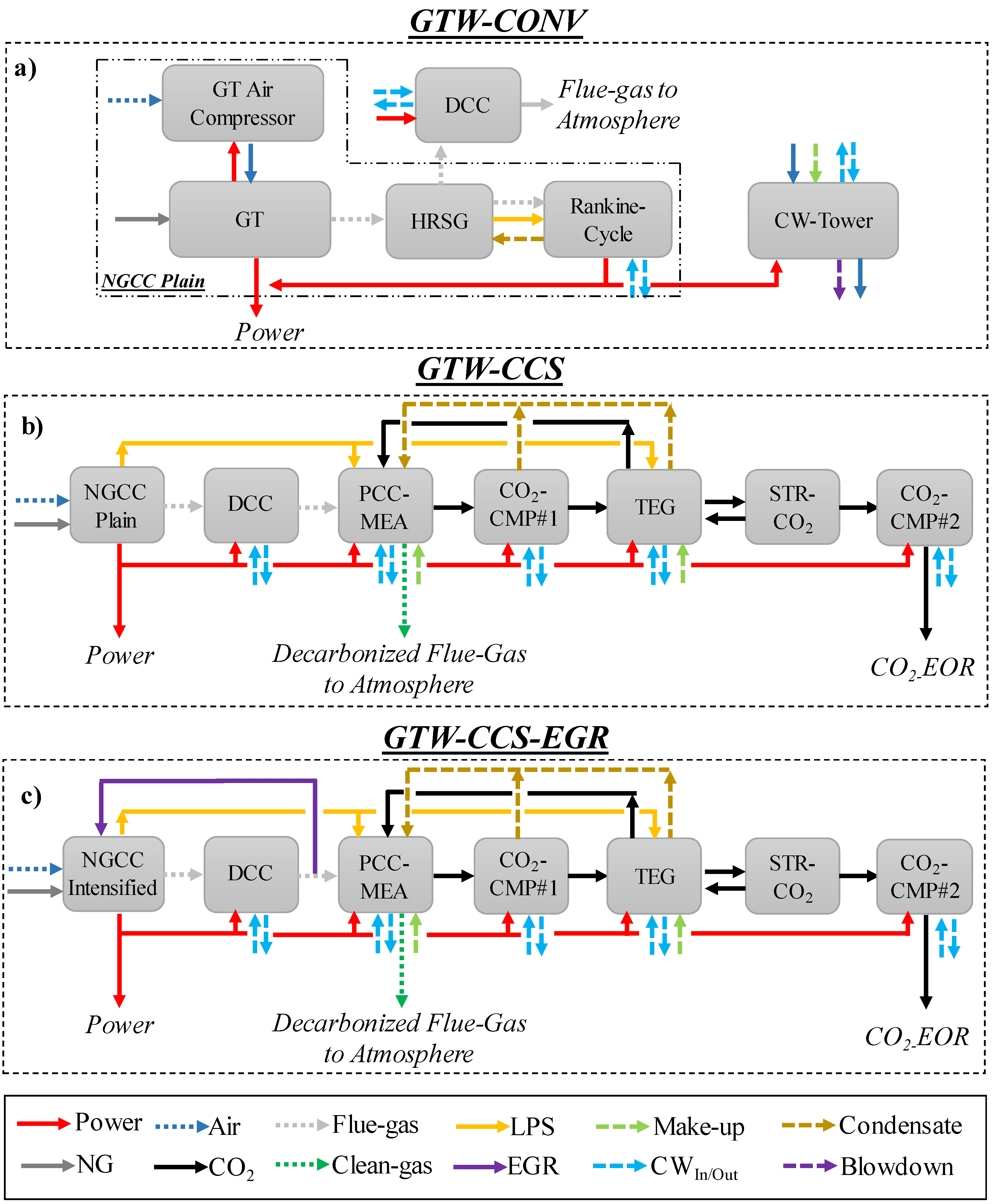
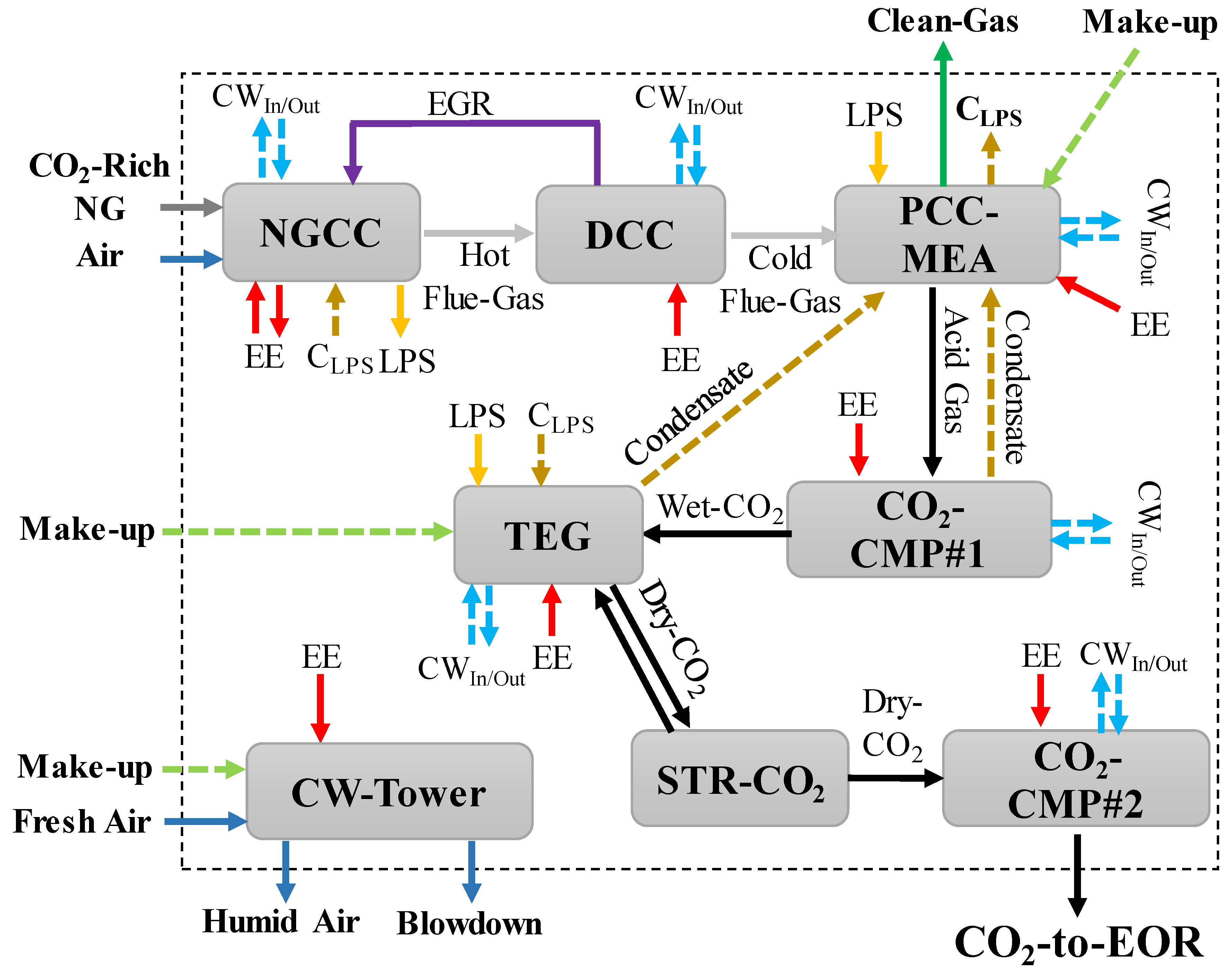
2.1. GTW-CONV, GTW-CCS, and GTW-CCS-EGR
2.2. Sub-Systems
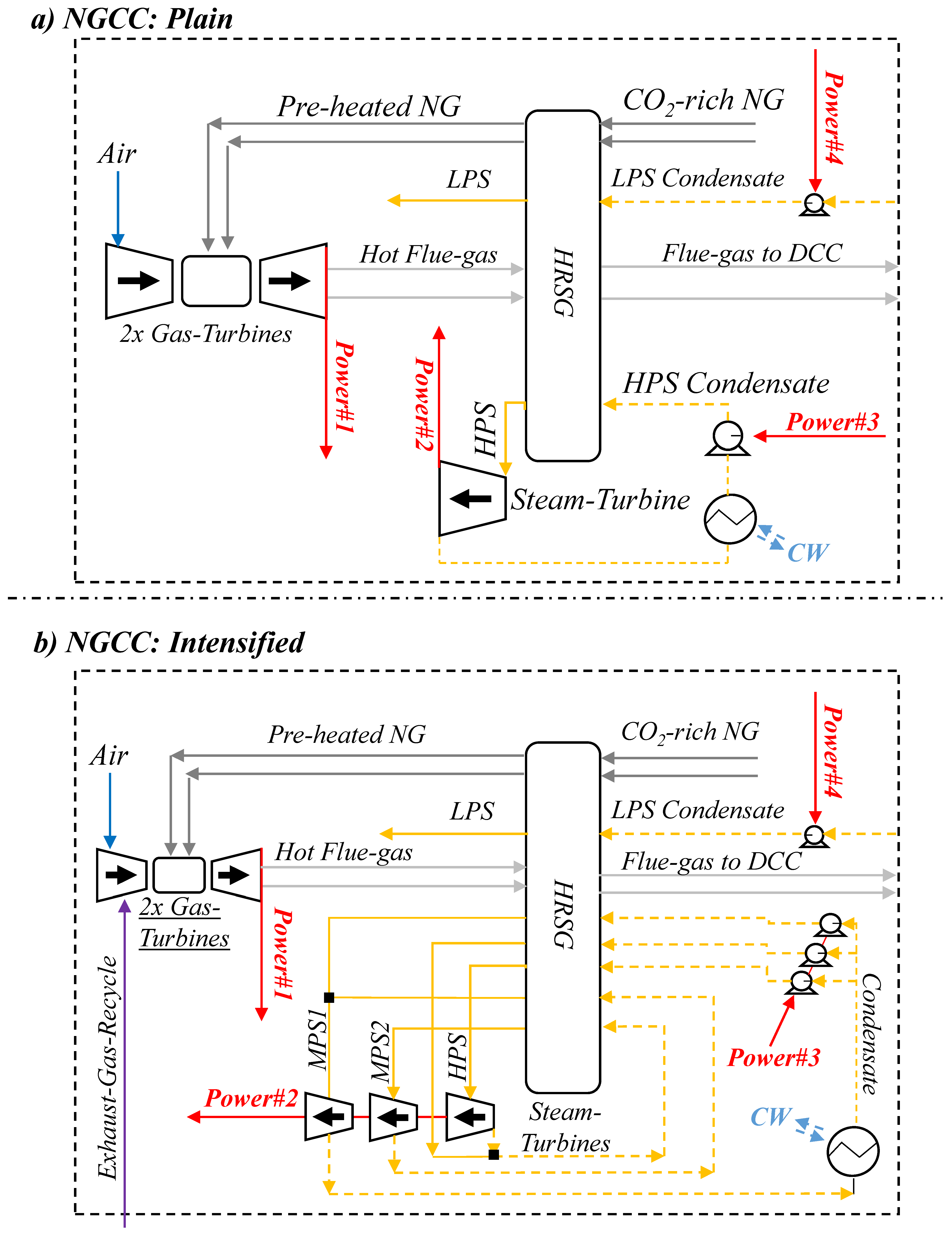
2.2.1. NGCC
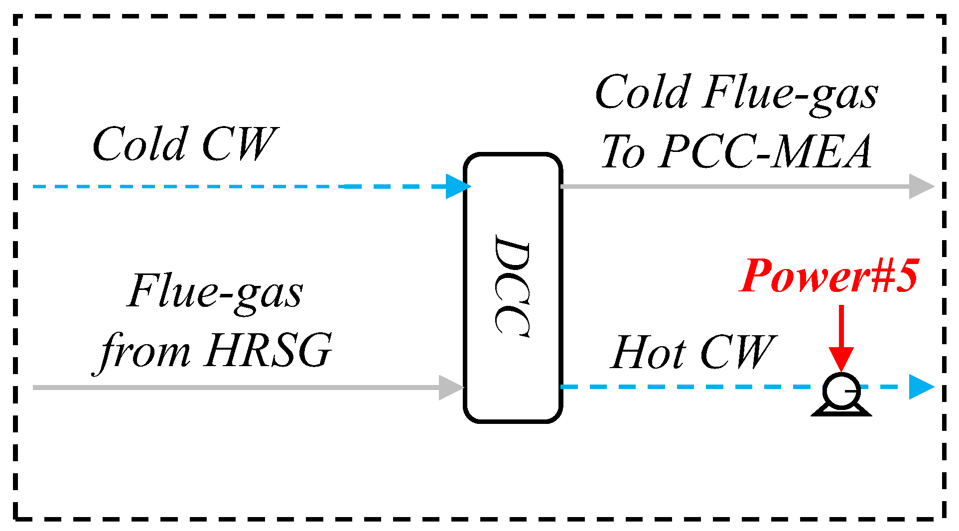
2.2.2. Direct Contact Column
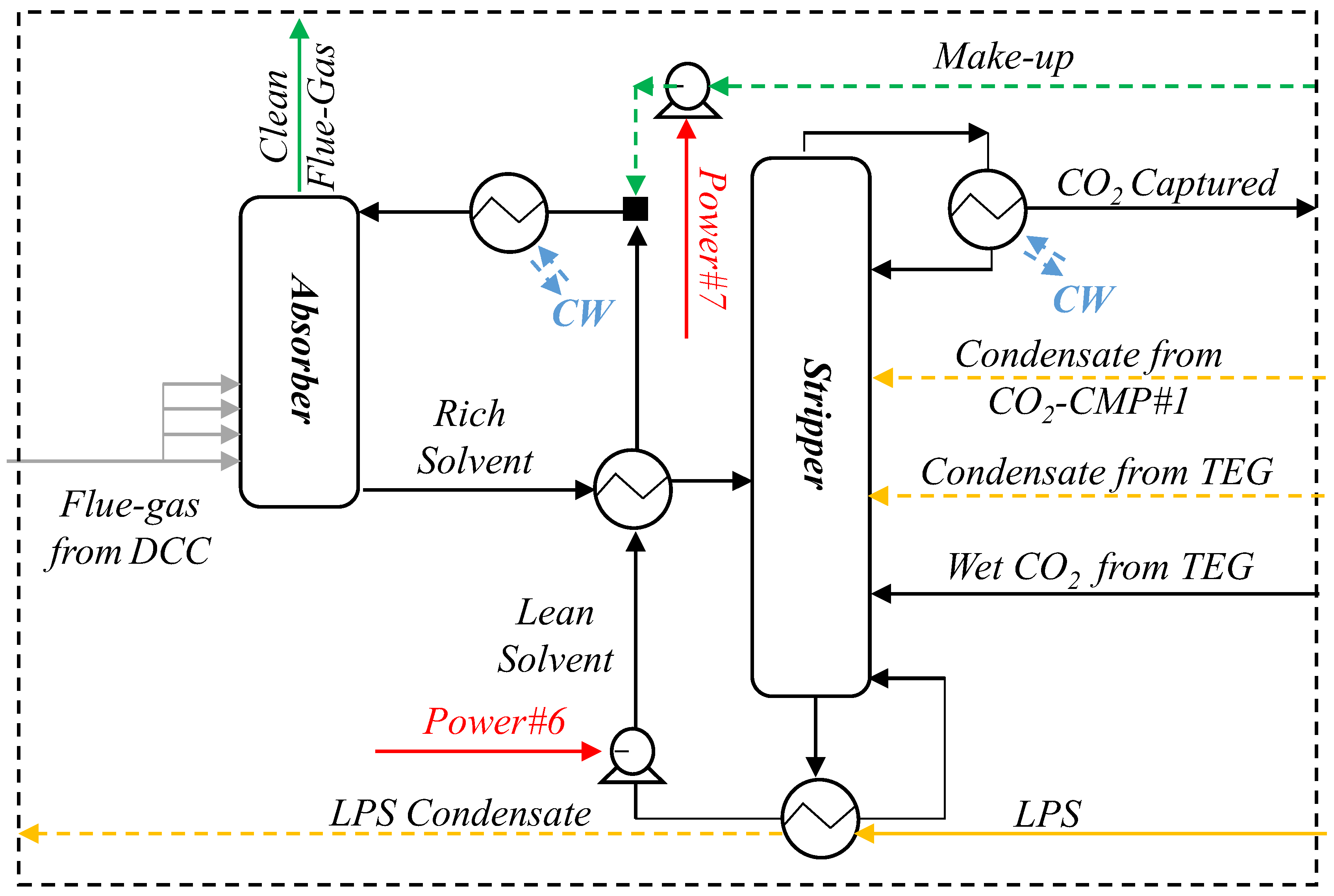
2.2.3. PCC-MEA
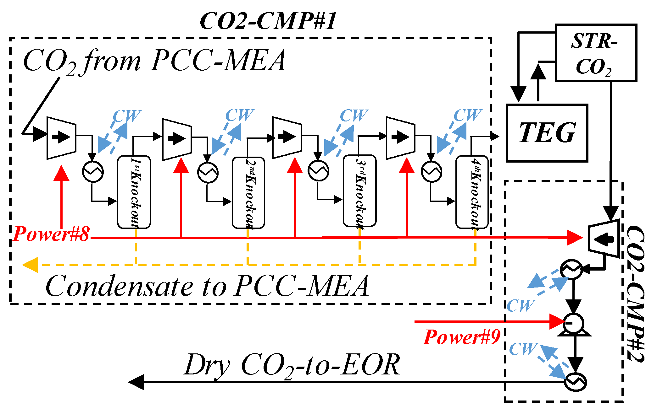
2.2.4. CO2 Compression (CO2-CMP)
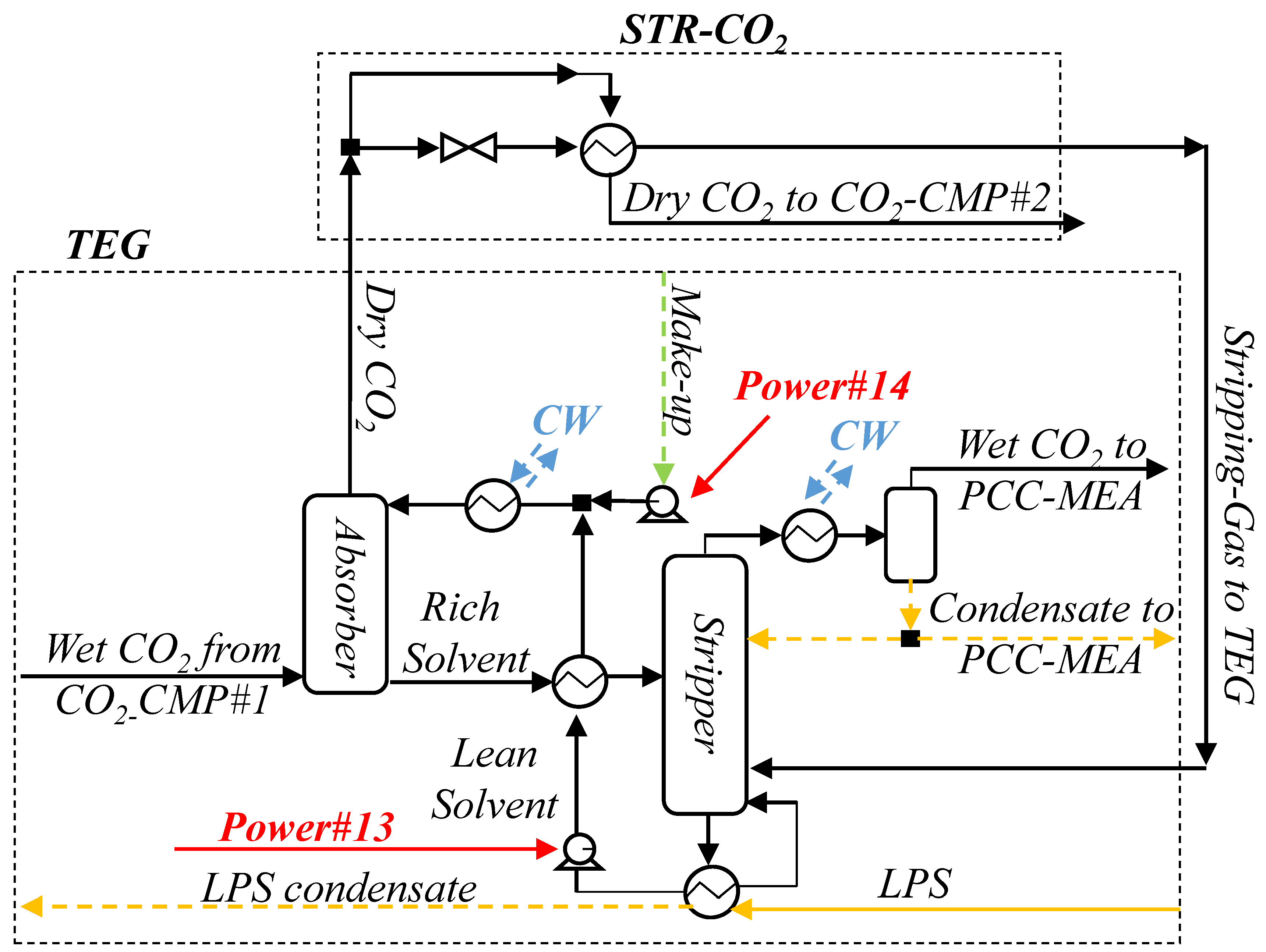
2.2.5. TEG Dehydration Unit (TEG) and Stripping CO2 Unit (STR-CO2)
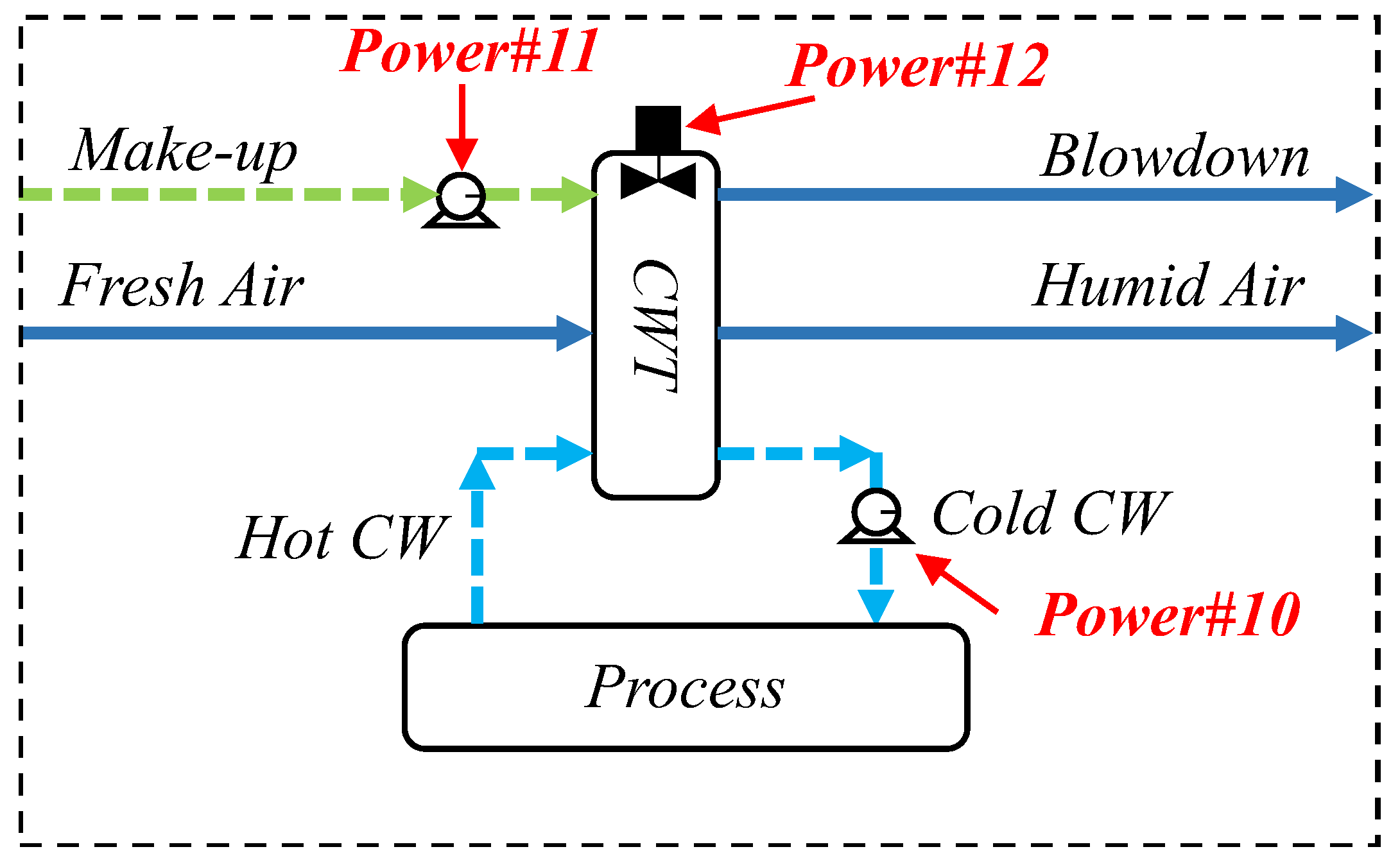
2.2.6. Cooling Water Tower
2.3. Economic Analysis
2.4. Multi-Criteria Sustainability Analysis
2.5. Thermodynamic Analysis of Processes
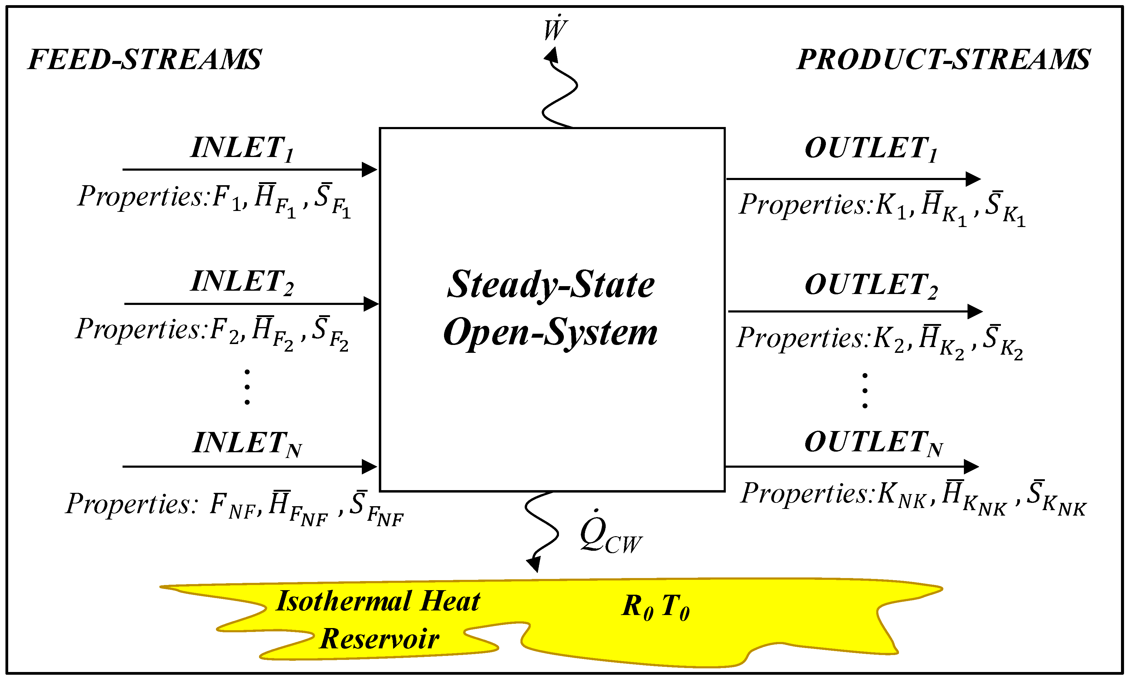
2.5.1. Maximum Work
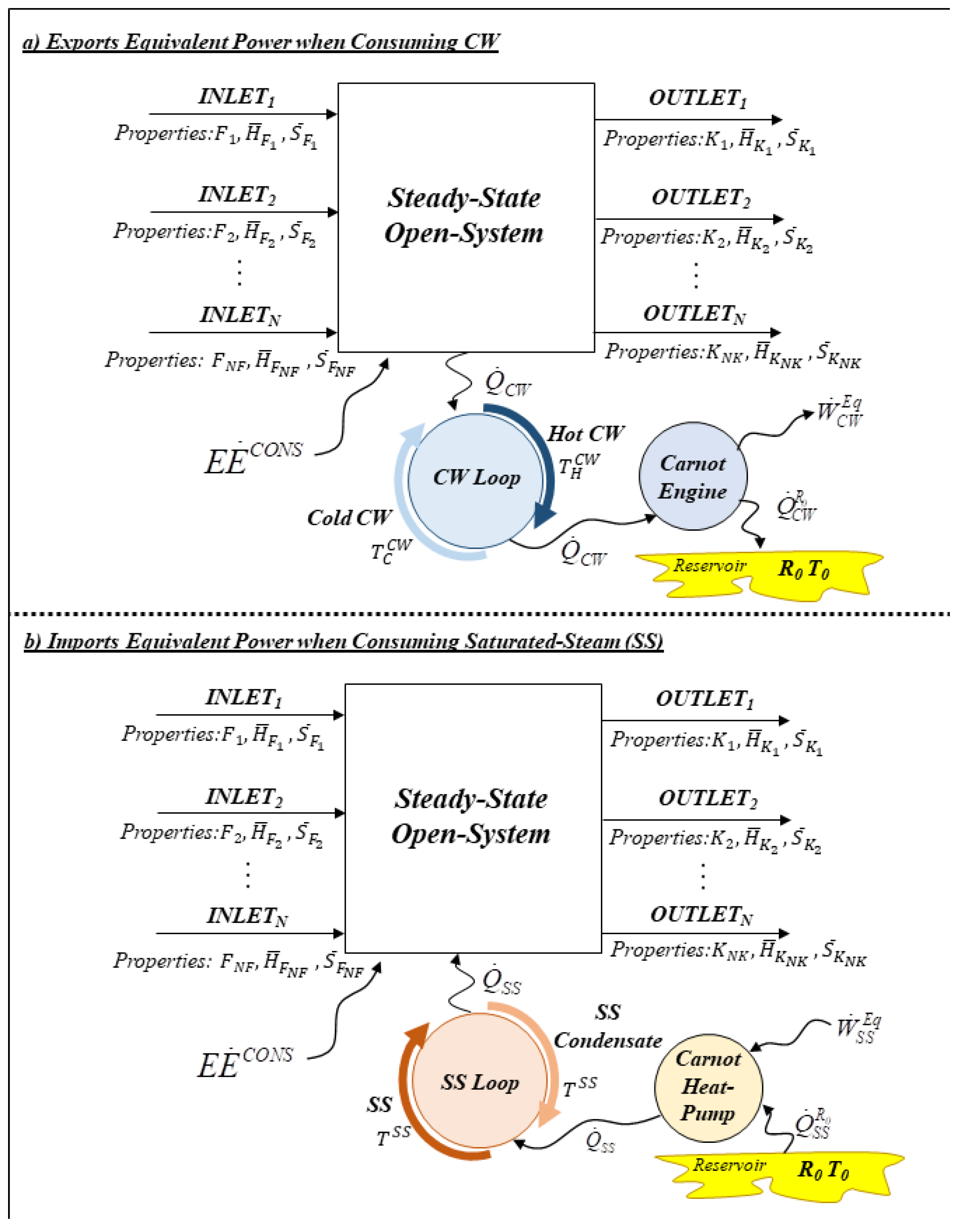
2.5.2. Equivalent Power
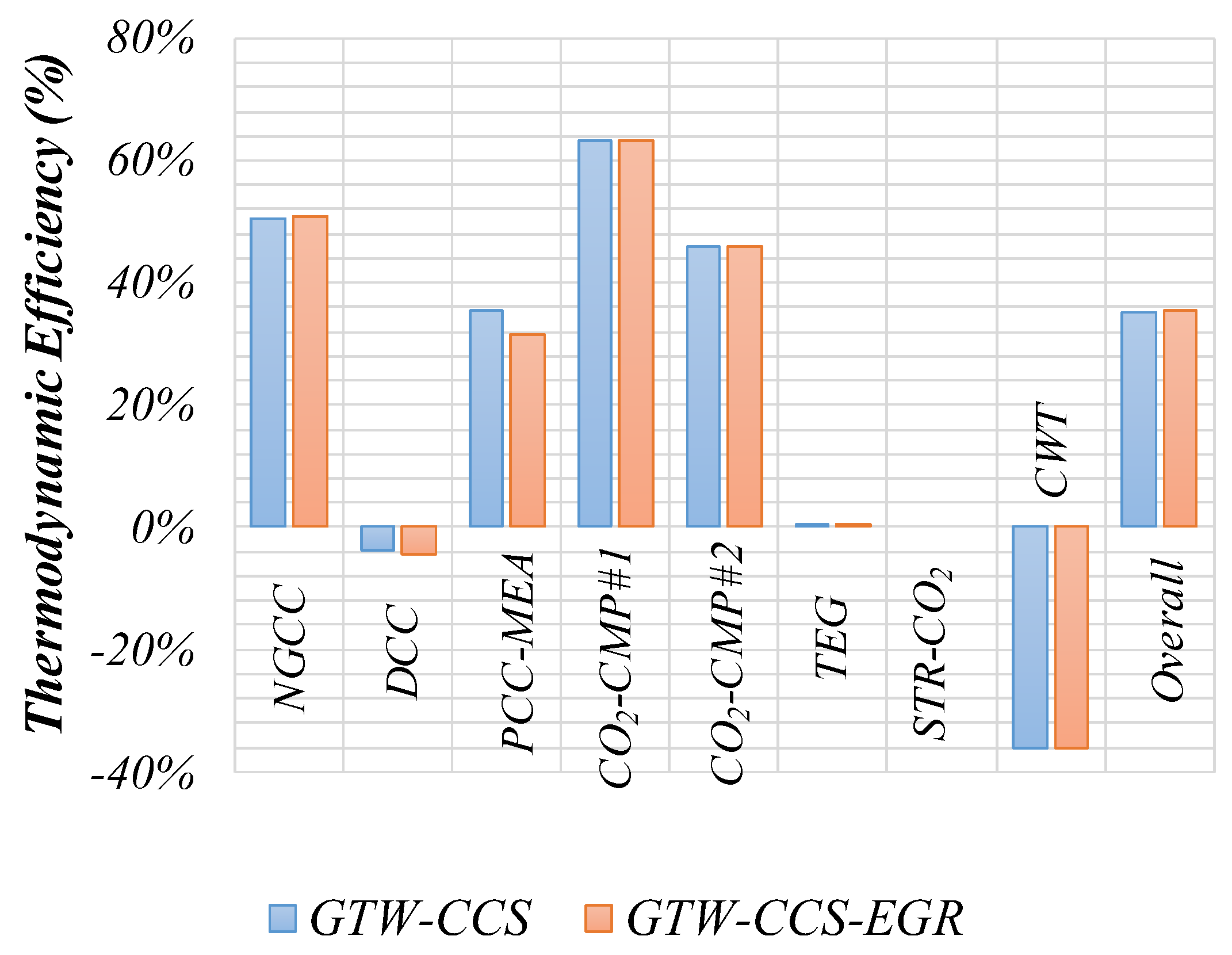
2.5.3. Thermodynamic Efficiency
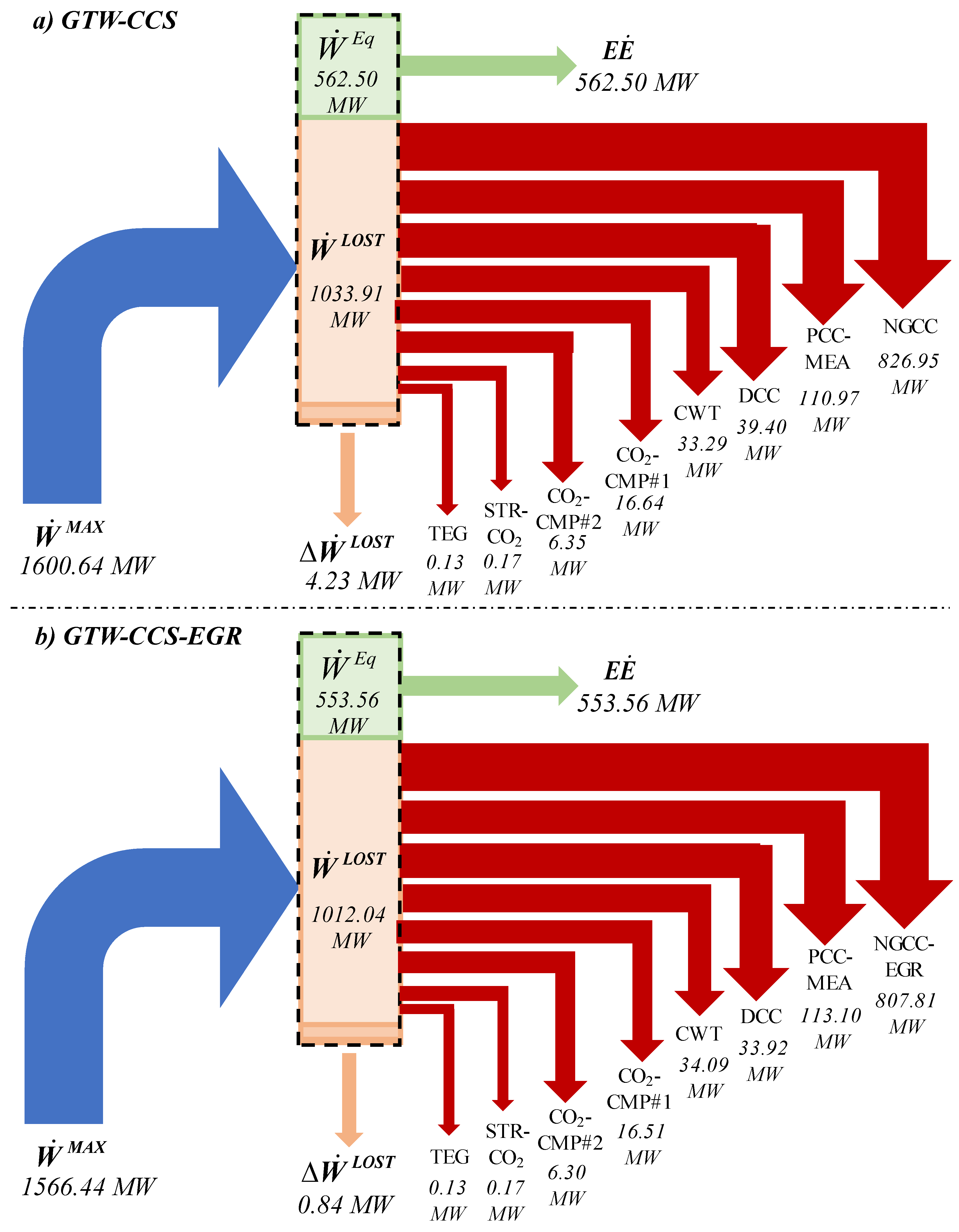
2.5.4. Lost Work
3. Results and Discussion
3.1. Technical Results
3.2. Multi-Criteria Sustainability Analysis Results
3.3. Thermodynamic Analysis Results
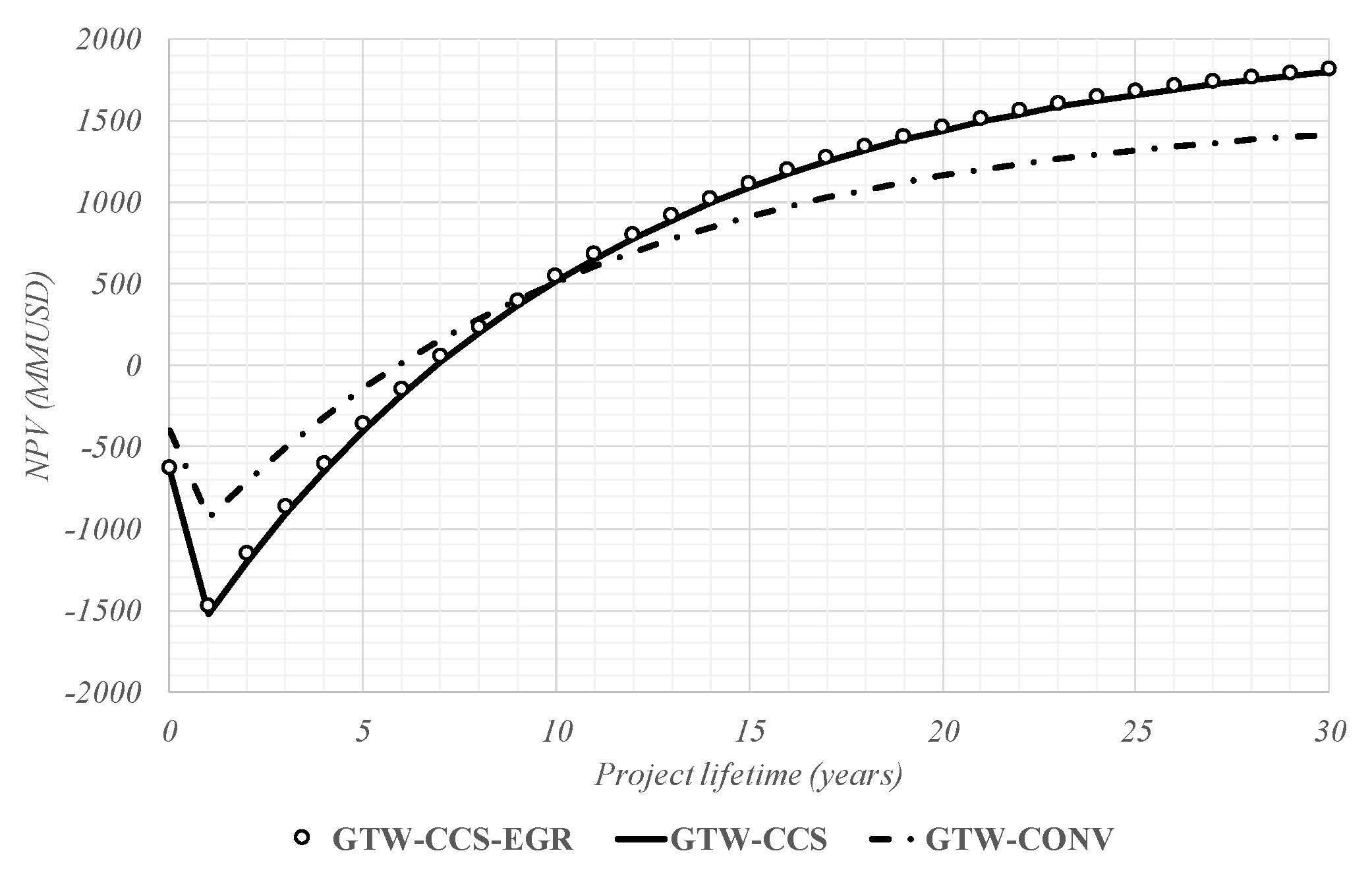
3.4. Economic Analysis
4. Conclusions
5. Suggestions for Future Work
Author Contributions
Funding
Data Availability Statement
Conflicts of Interest
Abbreviations
Nomenclature
| AP, GAP | Net and gross annual profits (MMUSD/y) |
| COL, COM | Costs of labor and of manufacturing (MMUSD/y) |
| CBM | Bare module costs (MMUSD) |
| CF | Capacity factor (MW, m2, or m3) |
| Isobaric heat capacity of water (J/mol.K) | |
| CEPCI | Chemical Engineering Plant Cost Index |
| CRM | Cost of raw materials (MMUSD/y) |
| CUT, DEPR | Cost of utilities and depreciation (MMUSD/y) |
| DPBP | Discounted Payback Time (y) |
| Electricity (MW) | |
| Fn | nth Feed stream flow rate (kmol/s) |
| FCI | Fixed Capital Investment (MMUSD) |
| Molar enthalpy (MJ/kmol) | |
| HR | Heat Ratio (kJ/kgCO2) |
| ITR, i | Income tax rate, annual interest rate (%) |
| NEQ | Number of equipment items |
| NF, NK | Numbers of feed streams and product streams |
| NPV | Net present value (MMUSD) |
| Kn | nth product stream flow rate (kmol/s) |
| Heat duty (MW) | |
| REV | Revenues (MMUSD/y) |
| Molar entropy (MJ/kmol.K) | |
| T | Absolute temperature (K) |
| Power (MW) | |
| η | Thermodynamic efficiency (%) |
References
- Kotagodahetti, R.; Hewage, K.; Perera, P.; Sadiq, R. Technology and Policy Options for Decarbonizing the Natural Gas Industry: A Critical Review. Gas Sci. Eng. 2023, 114, 204981. [Google Scholar] [CrossRef]
- United Nations Framework Convention on Climate Change (UNFCCC). Kyoto Protocol to the UNFCCC. Available online: https://unfccc.int/resource/docs/convkp/kpeng.pdf (accessed on 13 February 2024).
- Ellerman, A.D.; Buchner, B.K. The European Union Emissions Trading Scheme: Origins, Allocation, and Early Results. Rev. Environ. Econ. Policy 2007, 1, 66–87. [Google Scholar] [CrossRef]
- United Nations Framework Convention on Climate Change (UNFCCC). Paris Agreement. Available online: https://unfccc.int/sites/default/files/english_paris_agreement.pdf (accessed on 13 February 2024).
- Budinis, S.; Krevor, S.; Dowell, N.M.; Brandon, N.; Hawkes, A. An Assessment of CCS Costs, Barriers and Potential. Energy Strateg. Rev. 2018, 22, 61–81. [Google Scholar] [CrossRef]
- Guo, J.-X.; Huang, C.; Wang, J.-L.; Meng, X.-Y. Integrated Operation for the Planning of CO2 Capture Path in CCS–EOR Project. J. Pet. Sci. Eng. 2020, 186, 106720. [Google Scholar] [CrossRef]
- Rao, A.D. Natural Gas-Fired Combined Cycle (NGCC) Systems. In Combined Cycle Systems for Near-Zero Emission Power Generation; Elsevier: Amsterdam, The Netherlands, 2012; pp. 103–128. ISBN 978-0-85709-013-3. [Google Scholar]
- Hekmatmehr, H.; Esmaeili, A.; Pourmahdi, M.; Atashrouz, S.; Abedi, A.; Ali Abuswer, M.; Nedeljkovic, D.; Latifi, M.; Farag, S.; Mohaddespour, A. Carbon Capture Technologies: A Review on Technology Readiness Level. Fuel 2024, 363, 130898. [Google Scholar] [CrossRef]
- Carapellucci, R.; Giordano, L.; Vaccarelli, M. Study of a Natural Gas Combined Cycle with Multi-Stage Membrane Systems for CO2 Post-Combustion Capture. Energy Procedia 2015, 81, 412–421. [Google Scholar] [CrossRef]
- Khan, B.A.; Ullah, A.; Saleem, M.W.; Khan, A.N.; Faiq, M.; Haris, M. Energy Minimization in Piperazine Promoted MDEA-Based CO2 Capture Process. Sustainability 2020, 12, 8524. [Google Scholar] [CrossRef]
- Ab Rahim, A.H.; Yunus, N.M.; Bustam, M.A. Ionic Liquids Hybridization for Carbon Dioxide Capture: A Review. Molecules 2023, 28, 7091. [Google Scholar] [CrossRef] [PubMed]
- Grasa, G.S.; Abanades, J.C. CO2 Capture Capacity of CaO in Long Series of Carbonation/Calcination Cycles. Ind. Eng. Chem. Res. 2006, 45, 8846–8851. [Google Scholar] [CrossRef]
- Theo, W.L.; Lim, J.S.; Hashim, H.; Mustaffa, A.A.; Ho, W.S. Review of Pre-Combustion Capture and Ionic Liquid in Carbon Capture and Storage. Appl. Energy 2016, 183, 1633–1663. [Google Scholar] [CrossRef]
- Darabkhani, H.G.; Varasteh, H.; Bazooyar, B. Oxyturbine Power Cycles and Gas-CCS Technologies. In Carbon Capture Technologies for Gas-Turbine-Based Power Plants; Darabkhani, H.G., Varasteh, H., Eds.; Elsevier: Amsterdam, The Netherlands, 2023; pp. 39–74. ISBN 978-0-12-818868-2. [Google Scholar]
- Davoodi, S.; Al-Shargabi, M.; Wood, D.A.; Rukavishnikov, V.S.; Minaev, K.M. Review of Technological Progress in Carbon Dioxide Capture, Storage, and Utilization. Gas Sci. Eng. 2023, 117, 205070. [Google Scholar] [CrossRef]
- Wang, M.; Lawal, A.; Stephenson, P.; Sidders, J.; Ramshaw, C. Post-Combustion CO2 Capture with Chemical Absorption: A State-of-the-Art Review. Chem. Eng. Res. Des. 2011, 89, 1609–1624. [Google Scholar] [CrossRef]
- Plaza, J.M.; Van Wagener, D.; Rochelle, G.T. Modeling CO2 Capture with Aqueous Monoethanolamine. Int. J. Greenh. Gas Control 2010, 4, 161–166. [Google Scholar] [CrossRef]
- Valenti, G.; Bonalumi, D.; Macchi, E. Energy and Exergy Analyses for the Carbon Capture with the Chilled Ammonia Process (CAP). Energy Procedia 2009, 1, 1059–1066. [Google Scholar] [CrossRef]
- Peeters, A.N.M.; Faaij, A.P.C.; Turkenburg, W.C. Techno-Economic Analysis of Natural Gas Combined Cycles with Post-Combustion CO2 Absorption, Including a Detailed Evaluation of the Development Potential. Int. J. Greenh. Gas Control 2007, 1, 396–417. [Google Scholar] [CrossRef]
- Tait, P.; Buschle, B.; Ausner, I.; Valluri, P.; Wehrli, M.; Lucquiaud, M. A Pilot-Scale Study of Dynamic Response Scenarios for the Flexible Operation of Post-Combustion CO2 Capture. Int. J. Greenh. Gas Control 2016, 48, 216–233. [Google Scholar] [CrossRef]
- Schach, M.-O.; Schneider, R.; Schramm, H.; Repke, J.-U. Techno-Economic Analysis of Postcombustion Processes for the Capture of Carbon Dioxide from Power Plant Flue Gas. Ind. Eng. Chem. Res. 2010, 49, 2363–2370. [Google Scholar] [CrossRef]
- Luo, X.; Wang, M. Optimal Operation of MEA-Based Post-Combustion Carbon Capture for Natural Gas Combined Cycle Power Plants under Different Market Conditions. Int. J. Greenh. Gas Control 2016, 48, 312–320. [Google Scholar] [CrossRef]
- Bao, J.; Zhang, L.; Song, C.; Zhang, N.; Guo, M.; Zhang, X. Reduction of Efficiency Penalty for a Natural Gas Combined Cycle Power Plant with Post-Combustion CO2 Capture: Integration of Liquid Natural Gas Cold Energy. Energy Convers. Manag. 2019, 198, 111852. [Google Scholar] [CrossRef]
- Cormos, C.-C. Assessment of Chemical Absorption/Adsorption for Post-Combustion CO2 Capture from Natural Gas Combined Cycle (NGCC) Power Plants. Appl. Therm. Eng. 2015, 82, 120–128. [Google Scholar] [CrossRef]
- Garcia, S.; Fernandez, E.S.; Stewart, A.J.; Maroto-Valer, M.M. Process Integration of Post-Combustion CO2 Capture with Li4SiO4/Li2CO3 Looping in a NGCC Plant. Energy Procedia 2017, 114, 2611–2617. [Google Scholar] [CrossRef]
- Zhang, W.; Sun, C.; Snape, C.E.; Sun, X.; Liu, H. Cyclic Performance Evaluation of a Polyethylenimine/Silica Adsorbent with Steam Regeneration Using Simulated NGCC Flue Gas and Actual Flue Gas of a Gas-Fired Boiler in a Bubbling Fluidized Bed Reactor. Int. J. Greenh. Gas Control 2020, 95, 102975. [Google Scholar] [CrossRef]
- Roussanaly, S.; Aasen, A.; Anantharaman, R.; Danielsen, B.; Jakobsen, J.; Heme-De-Lacotte, L.; Neji, G.; Sødal, A.; Wahl, P.E.; Vrana, T.K.; et al. Offshore Power Generation with Carbon Capture and Storage to Decarbonise Mainland Electricity and Offshore Oil and Gas Installations: A Techno-Economic Analysis. Appl. Energy 2019, 233–234, 478–494. [Google Scholar] [CrossRef]
- Brito, T.L.F.; Galvão, C.; Fonseca, A.F.; Costa, H.K.M.; Moutinho dos Santos, E. A Review of Gas-to-Wire (GtW) Projects Worldwide: State-of-Art and Developments. Energy Policy 2022, 163, 112859. [Google Scholar] [CrossRef]
- Flórez-Orrego, D.; Albuquerque, C.; da Silva, J.A.M.; Freire, R.L.A.; de Oliveira Junior, S. Optimal Design of Power Hubs for Offshore Petroleum Platforms. Energy 2021, 235, 121353. [Google Scholar] [CrossRef]
- Orisaremi, K.K.; Chan, F.T.S.; Chung, N.S.H. Potential Reductions in Global Gas Flaring for Determining the Optimal Sizing of Gas-to-Wire (GTW) Process: An Inverse DEA Approach. J. Nat. Gas Sci. Eng. 2021, 93, 103995. [Google Scholar] [CrossRef]
- Jokar, S.M.; Wood, D.A.; Sinehbaghizadeh, S.; Parvasi, P.; Javanmardi, J. Transformation of Associated Natural Gas into Valuable Products to Avoid Gas Wastage in the Form of Flaring. J. Nat. Gas Sci. Eng. 2021, 94, 104078. [Google Scholar] [CrossRef]
- Henningsen, S. Air Pollution from Large Two-Stroke Diesel Engines and Technologies to Control It. In Handbook of Air Pollution from Internal Combustion Engines; Sher, E.B.T.-H., Ed.; Elsevier: San Diego, CA, USA, 1998; pp. 477–534. ISBN 978-0-12-639855-7. [Google Scholar]
- Okubo, M.; Kuwahara, T. Principle and Design of Emission Control Systems. In New Technologies for Emission Control in Marine Diesel Engines; Okubo, M., Kuwahara, T.B.T.-N.T., Eds.; Elsevier: Amsterdam, The Netherlands, 2020; pp. 53–143. ISBN 978-0-12-812307-2. [Google Scholar]
- Alcaráz-Calderon, A.M.; González-Díaz, M.O.; Mendez, Á.; González-Santaló, J.M.; González-Díaz, A. Natural Gas Combined Cycle with Exhaust Gas Recirculation and CO2 Capture at Part-Load Operation. J. Energy Inst. 2019, 92, 370–381. [Google Scholar] [CrossRef]
- Hachem, J.; Schuhler, T.; Orhon, D.; Cuif-Sjostrand, M.; Zoughaib, A.; Molière, M. Exhaust Gas Recirculation Applied to Single-Shaft Gas Turbines: An Energy and Exergy Approach. Energy 2022, 238, 121656. [Google Scholar] [CrossRef]
- Ali, U.; Agbonghae, E.O.; Hughes, K.J.; Ingham, D.B.; Ma, L.; Pourkashanian, M. Techno-Economic Process Design of a Commercial-Scale Amine-Based CO2 Capture System for Natural Gas Combined Cycle Power Plant with Exhaust Gas Recirculation. Appl. Therm. Eng. 2016, 103, 747–758. [Google Scholar] [CrossRef]
- Lee, W.-S.; Kang, J.-H.; Lee, J.-C.; Lee, C.-H. Enhancement of Energy Efficiency by Exhaust Gas Recirculation with Oxygen-Rich Combustion in a Natural Gas Combined Cycle with a Carbon Capture Process. Energy 2020, 200, 117586. [Google Scholar] [CrossRef]
- Nanadegani, F.S.; Sunden, B. Review of Exergy and Energy Analysis of Fuel Cells. Int. J. Hydrogen Energy 2023, 48, 32875–32942. [Google Scholar] [CrossRef]
- Nie, X.; Xue, J.; Zhao, L.; Deng, S.; Xiong, H. New Insight of Thermodynamic Cycle in Thermoelectric Power Generation Analyses: Literature Review and Perspectives. Energy 2024, 292, 130553. [Google Scholar] [CrossRef]
- Geuzebroek, F.H.; Schneiders, L.H.J.M.; Kraaijveld, G.J.C.; Feron, P.H.M. Exergy Analysis of Alkanolamine-Based CO2 Removal Unit with AspenPlus. Energy 2004, 29, 1241–1248. [Google Scholar] [CrossRef]
- Gülen, S.C.; Smith, R.W. Second Law Efficiency of the Rankine Bottoming Cycle of a Combined Cycle Power Plant. J. Eng. Gas Turbines Power 2010, 132, 011801. [Google Scholar] [CrossRef]
- Brigagão, G.V.; Arinelli, L.D.O.; de Medeiros, J.L.; Araújo, O.d.Q.F. Low-Pressure Supersonic Separator with Finishing Adsorption: Higher Exergy Efficiency in Air Pre-Purification for Cryogenic Fractionation. Sep. Purif. Technol. 2020, 248, 116969. [Google Scholar] [CrossRef]
- Cruz, M.D.A.; de Araújo, O.Q.F.; de Medeiros, J.L. Exergy Comparison of Single-Shaft and Multiple-Paralleled Compressor Schemes in Offshore Processing of CO2-Rich Natural Gas. J. Nat. Gas Sci. Eng. 2020, 81, 103390. [Google Scholar] [CrossRef]
- Wiesberg, I.L.; Brigagão, G.V.; Araújo, O.D.Q.F.; de Medeiros, J.L. Carbon Dioxide Management via Exergy-Based Sustainability Assessment: Carbon Capture and Storage versus Conversion to Methanol. Renew. Sustain. Energy Rev. 2019, 112, 720–732. [Google Scholar] [CrossRef]
- Milão, R.D.F.D.; Carminati, H.B.; de Araújo, O.Q.F.; de Medeiros, J.L. Thermodynamic, Financial and Resource Assessments of a Large-Scale Sugarcane-Biorefinery: Prelude of Full Bioenergy Carbon Capture and Storage Scenario. Renew. Sustain. Energy Rev. 2019, 113, 109251. [Google Scholar] [CrossRef]
- Talebizadehsardari, P.; Ehyaei, M.A.; Ahmadi, A.; Jamali, D.H.; Shirmohammadi, R.; Eyvazian, A.; Ghasemi, A.; Rosen, M.A. Energy, Exergy, Economic, Exergoeconomic, and Exergoenvironmental (5E) Analyses of a Triple Cycle with Carbon Capture. J. CO2 Util. 2020, 41, 101258. [Google Scholar] [CrossRef]
- Amrollahi, Z.; Ertesvåg, I.S.; Bolland, O. Optimized Process Configurations of Post-Combustion CO2 Capture for Natural-Gas-Fired Power Plant—Exergy Analysis. Int. J. Greenh. Gas Control 2011, 5, 1393–1405. [Google Scholar] [CrossRef]
- Minutillo, M.; Lubrano Lavadera, A.; Jannelli, E. Assessment of Design and Operating Parameters for a Small Compressed Air Energy Storage System Integrated with a Stand-Alone Renewable Power Plant. J. Energy Storag. 2015, 4, 135–144. [Google Scholar] [CrossRef]
- Souza, I.V.A.F.; Ellis, G.S.; Ferreira, A.A.; Guzzo, J.V.P.; Díaz, R.A.; Albuquerque, A.L.S.; Amrani, A. Geochemical Characterization of Natural Gases in the Pre-Salt Section of the Santos Basin (Brazil) Focused on Hydrocarbons and Volatile Organic Sulfur Compounds. Mar. Pet. Geol. 2022, 144, 105763. [Google Scholar] [CrossRef]
- General Electric (GE). GE Gas&Power—Gas Turbines 9F. Available online: https://www.ge.com/gas-power/products/gas-turbines/9f (accessed on 13 February 2024).
- Turton, R. Analysis, Synthesis, and Design of Chemical Processes; Prentice-Hall International Series in Engineering; Prentice Hall: Hoboken, NJ, USA, 2012; ISBN 9780132618120. [Google Scholar]
- Chemical Engineering (CE). The Chemical Engineering Plant Cost Index. Available online: https://www.chemengonline.com/Assets/File/CEPCI_2002.pdf (accessed on 13 February 2024).
- Carminati, H.B.; Milão, R.D.F.D.; de Medeiros, J.L.; de Araújo, O.Q.F. Bioenergy and Full Carbon Dioxide Sinking in Sugarcane-Biorefinery with Post-Combustion Capture and Storage: Techno-Economic Feasibility. Appl. Energy 2019, 254, 113633. [Google Scholar] [CrossRef]
- U.S. Energy Information Administration (EIA). Natural Gas Henry Hub Spot Price: Average of 2022. Available online: https://www.eia.gov/dnav/ng/hist/rngwhhdm.htm (accessed on 13 February 2024).
- U.S. Energy Information Administration (EIA). Independent Statistics and Analysis. Electricity and Natural Gas Data Browser: Average of 2022. Available online: https://www.eia.gov/electricity/data/browser/#/topic/7?agg=2,0,1&geo=g&freq=M (accessed on 13 February 2024).
- Thorne, R.J.; Sundseth, K.; Bouman, E.; Czarnowska, L.; Mathisen, A.; Skagestad, R.; Stanek, W.; Pacyna, J.M.; Pacyna, E.G. Technical and Environmental Viability of a European CO2 EOR System. Int. J. Greenh. Gas Control 2020, 92, 102857. [Google Scholar] [CrossRef]
- Liptak, B. Optimization of Cooling Towers. Available online: https://www.controlglobal.com/manage/optimization/article/11304737/optimization-of-cooling-towers (accessed on 13 February 2024).
- Ruiz-Mercado, G.J.; Smith, R.L.; Gonzalez, M.A. Sustainability Indicators for Chemical Processes: I. Taxonomy. Ind. Eng. Chem. Res. 2012, 51, 2309–2328. [Google Scholar] [CrossRef]
- Aspentech. 2024. Aspen Technology Inc. Available online: www.aspentech.com/en/about-aspentech (accessed on 1 March 2024).
- Mcampbell, J. Gas Conditioning and Processing. J. Chem. Inf. Model. 2013, 53, 1689–1699. [Google Scholar]
- Kim, S. Maximum Allowable Fluid Velocity and Concern on Piping Stability of ITER Tokamak Cooling Water System. Fusion Eng. Des. 2021, 162, 112049. [Google Scholar] [CrossRef]


| (a) | ||
| Item | Description | Assumptions |
| A1 | NG-to-onshore Compressor | Compression RatioStage = 1.6; Stages = 4; TIntercooler = 40 °C; PInlet = 30 bar; POutlet = 200 bar; TOutlet = 40 °C [43] |
| A2 | Molecular Sieve Temperature Swing Adsorption | PInlet = 75 bar; Dehydration Target: H2O = 1 ppm-mol; Adsorption Cycle = 12 h; Regeneration Cycle = 4 h; MassAdsorbent = 50,000 kg/Vessel; Vessels = 2; DensityAdsorbent = 800 kg/m3; WaterAdsorbed = 0.1 kgWater/kgAdsorbent [42]; |
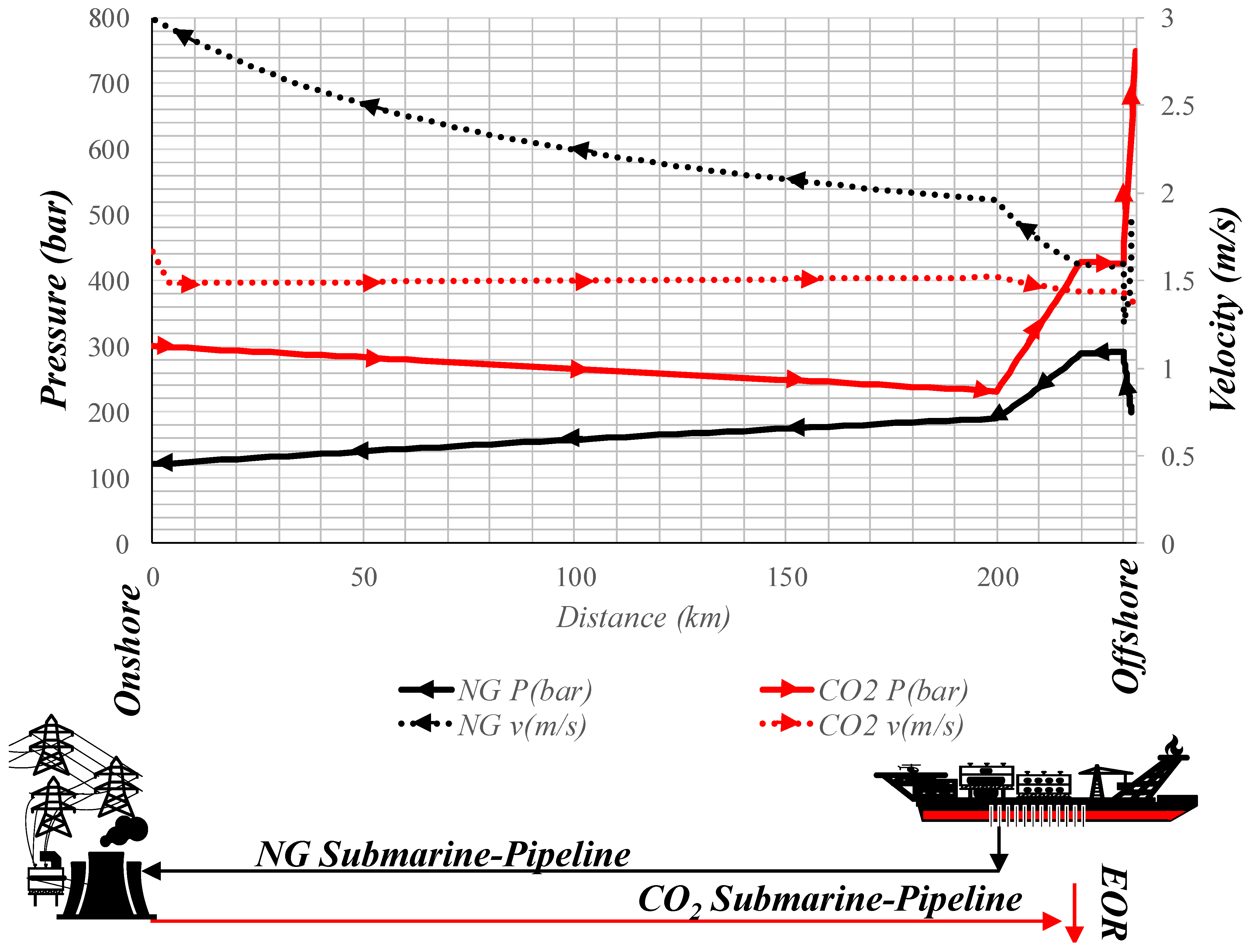
| A3 | NG Downcomer | PInlet = 200 bar; Flexible Pipes = 2; Inner Diameter = 12″; Length = 2000 m; Inclination = −100%; Average TExternal = 15 °C [45]. |
| A4 | NG Pipeline Rig-to-Shore | Inner Diameter = 16″; Max Velocity = 3 m/s; POutlet ≥ 70 bar; Segment-1: Length = 10 km; Inclination = +0.1%; Average TExternal = 5 °C; Segment-2: Length = 20 km; Inclination = +10%; Average TExternal = 10 °C; Segment-3: Length = 200 km; Inclination = +0.1%; Average TExternal = 20 °C [45]. |
| (b) | ||
| Item | Description | Assumptions |
| A5 | Thermodynamic Modeling | Base Model: PR-EOS; PCC-MEA: HYSYS Acid–Gas Package; Pipelines: Beggs and Brill + PR-EOS [45]; CW + Rankine Cycle: HYSYS ASME Steam Table; TEG unit: Glycol Package. |
| A6 | Treated CO2-Rich NG | 6.5 MMm3,Std/d; T = 40 °C; P = 18.5 bar; CO2 = 44% mol, CH4 = 50% mol, C2H6 = 3% mol, C3H8 = 2% mol, C4H10 = 1% mol, H2O = 1 ppm-mol [49]. |
| A7 | CW | TInlet = 35 °C; TOutlet = 55 °C; PInlet = 4 bar; POutlet = 3.5 bar [43]. |
| A8 | Adiabatic Efficiencies | ηPumps = 75%; ηSteam Turbine = 85%; η Compressors = 75%; η CWT Blower = 95%; Gas Turbine: ηAir Compressor = 87%; ηExpander = 90% [42]. |
| A9 | Heat Exchangers | ΔP = 0.5 bar; Thermal Approaches: ΔTGas-CW = 5 °C, ΔTGas-Gas = 10 °C, ΔTLiq-Liq = 5 °C [43]. |
| A10 | Steam Streams HPS, MPS1, MPS2, LPS (saturated) | GTW-CONV and GTW-CCS: PHPS = 45 bar; THPS = 545 °C; PLPS = 3 bar; TLPS = 135 °C; GTW-CCS-EGR: PHPS = 90 bar, THPS = 535 °C; PMPS1 = 21 bar, TMPS1 = 535 °C; PMPS2 = 3.8 bar, TMPS2 = 343 °C; PLPS = 4.7 bar, TLPS = 150 °C [45]. |
| A11 | HRSG | ΔTApproach = 50 °C; ΔPFlue Gas = 0.025 bar; ΔPSteam = 0.050 bar [45]. |
| A12 | Rankine Cycle | GTW-CONV and GTW-CCS: PHPS = 45 bar; POutlet = 0.25 bar; QualityOutlet = 95.1%; GTW-CCS-EGR: PHPS = 90 bar; PMPS1 = 21 bar; PMPS2 = 3.8 bar; POutlet = 0.16 bar; QualityOutlet = 99.1% [45]. |
| A13 | Air | T = 25 °C; P = 1 atm; N2 = 76.6% mol; O2 = 20.6% mol; H2O = 1.9% mol; Ar = 0.9% mol. |
| A14 | Gas Turbine (2 Gas Turbines) | GE9F.05; Air = 170.3 t/h; NG = 3.252 MMsm3/d; PInlet = 18 bar; TOUT = 640 °C [50]; GTW-CONV and GTW-CCS: Air = 14.2 kg/kgNG; GTW-CCS-EGR: Air = 6.5 kg/kgNG. |
| A15 | DCC | 4-Staged Tray Column; PTop = 1 bar; 36 °C [42] |
| A16 | PCC-MEA | Solvent: MEA = 29.9% w/w; H2O = 70.1% w/w; Heating Utility: LPS [45]; Absorber: 40-Staged, TSolvent Inlet = 36 °C; Stripper: 20-Staged, PCondenser = 1 bar, PReboiler = 1.3 bar, TSolvent Inlet = 90 °C, TCondenser = 40 °C, TReboiler = 110 °C. |
| A17 | CO2 Compression | Compression RatioStage = 2.7; Stages = 5; TIntercooler = 40 °C [43]. |
| A18 | TEG Unit | Lean TEG: TEG = 98.5% w/w; Absorber: PTop = 46.4 bar, TTEG Inlet = 40 °C; Stripper: PCondenser = 1 bar, TTEG Inlet = 75 °C, TCondenser = 40 °C, TReboiler = 140 °C; Absorber = 20-Staged; Stripper = 10-Staged; Dry-CO2:154 ppm-mol H2O. |
| A19 | CO2-to-EOR | P = 300 bar; T = 40 °C; CO2GTW-CCS = 99.6% mol; CO2GTW-CCS-EGR = 99.99% mol. |
| A20 | CW Tower | Blowdown = Evaporation; WaterMake-up: P = 1.013 bar, T = 30 °C; ∆PBlower = 2 kPa [45]. |
| A21 | Steam | Priority: LPS; Surplus: HPS/MPS1/MPS2. |
| A22 | EGR | Flue GasRecycle = 53.23%; AirInlet: Stoichiometric. |
| A23 | CO2 Pipeline Shore-to-Field | PInlet = 300 bar; POutlet ≥ 750 bar; Inner Diameter = 13″; Max Velocity = 3 m/s; Segment-1: Length = 200 km; Inclination = −0.1%; Average TExternal = 20 °C; Segment-2: Length = 20 km; Inclination = −10%; Average TExternal = 10 °C; Segment-3: Length = 10 km; Inclination = −0.1%; Average TExternal = 5 °C; Segment 4: Length = 3 km; Inclination = −100%; Average TExternal = 30 °C [45]. |
| System | Tributaries | Description |
|---|---|---|
| Gas Turbines | Power#1 | Power#1GTW-CCS > Power#1GTW-CCS-EGR |
| Steam Turbines | Power#2 | Power#2GTW-CONV > Power#2GTW-CCS-EGR > Power#2GTW-CCS |
| HPS condensate pump | Power#3 | Power#3GTW-CONV > Power#3GTW-CCS-EGR > Power#3GTW-CCS |
| LPS condensate pump | Power#4 | Power#4GTW-CCS > Power#4GTW-CCS-EGR |
| DCC pump | Power#5 | Power#5GTW-CONV = Power#5GTW-CCS = Power#5GTW-CCS-EGR |
| PCC-MEA recirculation pump | Power#6 | Power#6GTW-CCS > Power#6GTW-CCS-EGR |
| PCC-MEA make-up pump | Power#7 | Power#7GTW-CCS > Power#7GTW-CCS-EGR |
| CO2 Compressors | Power#8 | Power#8GTW-CCS > Power#8GTW-CCS-EGR |
| CO2-to-EOR pump | Power#9 | Power#9GTW-CCS ≈ Power#9GTW-CCS-EGR |
| CW Tower pump | Power#10 | Power#10GTW-CONV < Power#10GTW-CCS < Power#10GTW-CCS-EGR |
| CW Tower make-up pump | Power#11 | Power#11 GTW-CONV < Power#11GTW-CCS < Power#1 GTW-CCS-EGR |
| CW Tower blower | Power#12 | Power#1 GTW-CONV < Power#12GTW-CCS < Power#6GTW-CCS-EGR |
| TEG pump | Power#13 | - |
| TEG make-up pump | Power#14 | - |
| CW Tower GTW-CONV | PowerCWTGTW-CONV | Power#10 + Power#11 + Power#12 |
| CW Tower GTW-CCS | PowerCWTGTW-CCS | Power#10 + Power#11 + Power#12 |
| CW Tower GTW-CCS-EGR | PowerCWTGTW-CCS-EGR | Power#10 + Power#11 + Power#12 |
| PCC-MEA | PowerPCC-MEA | Power#6 + Power#7 |
| CO2-CMP | PowerCO2-CMP | Power#8 + Power#9 |
| GTW-CONV | PowerGTW-CONV | Power#1 + Power#2 − Power#3 − Power#5 − PowerCWTGTW-CONV |
| GTW-CCS | PowerGTW-CCS | Power#1 + Power#2 − Power#3-Power#4 − Power#5 − PowerPCC-MEA − Power#CO2-CMP − PowerCWTGTW-CCS |
| GTW-CCS-EGR | PowerGTW-CCS-EGR | Power#1 + Power#2 − Power#3 − Power#4 − Power#5 − PowerPCC-MEA − Power#CO2-CMP − PowerCWTGTW-CCS-EGR − Power#13 − Power#14 |
| Item | Parameter | Assumption |
|---|---|---|
| E1 | Operation lifetime (y) | 30 |
| E2 | Construction time (y) | 2 (40%/60%) |
| E3 | Operation (h/y) | 8400 |
| E4 | i (%) | 10 |
| E5 | DEPR (%FCI) | 10 |
| E6 | ITR (%) | 34 |
| E7 | NG price (USD/MMBTU) [54] | 2.82 |
| E8 | Electricity price (USD/kWh) [55] | 0.1026 |
| E11 | Labor cost (USD/y.operator) [51] | 89,100 |
| E12 | EOR yield (bblOil/tCO2) [56] | 1.5 |
| E13 | MEA Price (USD/kg) | 2 |
| E14 | Water Make-up Price (USD/m3) [45] | 0.0003 |
| E15 | FCI CW Tower (USD/GPM) [57] | 40 |
| E16 | Molecular Sieve (USD/kg) | 1.0 |
| E17 | NG Downcomer | 4 MMUSD/km |
| E18 | NG Pipeline (Segment 1) [53] | 4 MMUSD/km |
| E19 | NG Pipeline (Segment 2) [53] | 4 MMUSD/km |
| E20 | NG Pipeline (Segment 3) [53] | 3 MMUSD/km |
| E21 | CO2 Pipeline (Segment 1) [53] | 2 MMUSD/km |
| E22 | CO2 Pipeline (Segment 2) [53] | 3 MMUSD/km |
| E23 | CO2 Pipeline (Segment 3) [53] | 3 MMUSD/km |
| E24 | CO2 Pipeline (Segment 4) [53] | 3 MMUSD/km |
| Symbol | Definition | Unit | Best Case | Worst Case |
|---|---|---|---|---|
| Economic | ||||
| NPV | Net Present Value | USD | 0% interest | NPV = 0 |
| DPBP | Discounted Payback Periodfor NPV = 0 | y | DPBP = 3 | DPBP = 30 |
| TR | Turnover Ratio (Revenues/FCI) | USD/USD | TR = 4 | TR = 0 |
| COM | Cost of Manufacture | USD/y | COM = 0 | COM = Revenues |
| CRMv | Cost of Raw Material per Power Exported (Hourly) | USD/kWh | CRMv = 0 | Revenues/Power Exported |
| Environmental | ||||
| HS | No. of Hazardous Substance Inputs | - | HS = 0 | All inputs hazardous |
| HSs | Hazardous Substances Consumption per Power Exported | kg/kWh | HSs = 0 | All inputs hazardous |
| CI | CO2 Emitted per Power Exported | kg/kWh | CI = 0 | 100% CO2 emitted |
| CIv | CO2 Emitted per Revenues | kg/USD | CIv = 0 | 100% CO2 emitted |
| Material | ||||
| Mcp | Mass Input | kg | Equals MassOutput | 40 * MassOutput |
| MI | Mass Consumption per Power Exported | kg/kWh | 1 | 40 |
| WI | Water Consumption per Power Exported | m3/kWh | 0 | MI = WI |
| WIv | Water Consumption per Revenues | m3/USD | 0 | 1.55 |
| Energy | ||||
| Eff | Power Produced per Energy Input | kW/kW | 1 | 0 |
| Ecp | Energy Consumption | kW | 0 | Power Produced |
| ER | Power Demand per Power Exported | kW/kW | 0 | 1 |
| EU | Energy Required by Utilities | kW | 0 | 10% of Power Exported |
| Case | GTW-CONV | GTW-CCS | GTW-CCS-EGR | ||||
|---|---|---|---|---|---|---|---|
| Stream | NG Feed | Flue Gas | Clean Flue Gas | CO2-to-EOR | Flue Gas to PCC-MEA | Clean Flue Gas | CO2-to-EOR |
| T (°C) | 40 | 40 | 55 | 40 | 36.5 | 62.9 | 40 |
| P (bar) | 18.5 | 1 atm | 1 atm | 300 | 1.05 | 1 atm | 300 |
| Flow rate (kmol/h) | 11,459.8 | 181,869.1 | 176,135.0 | 11,623.3 | 79,530.5 | 78,143.2 | 11,496.1 |
| CH4 (% mol) | 50 | 0 | 0 | 0 | 0 | 0 | 0 |
| C2+ (% mol) | 6 | 0 | 0 | 0 | 0 | 0 | 0 |
| CO2 (% mol) | 44 | 7.21 | 0.59 | 99.64 | 15.80 | 1.37 | 99.95 |
| H2O (% mol) | ≈0 | 5.89 | 13.98 | 0.33 | 6.08 | 20.0 | 0.03 |
| N2 (% mol) | 0 | 74.36 | 73.86 | 0.03 | 77.22 | 78.6 | 0.02 |
| O2 (% mol) | 0 | 11.65 | 11.57 | 0 | 0 | 0 | 0 |
| H2 (% mol) | 0 | 0 | 0 | 0 | 0 | 0 | 0 |
| Ar (% mol) | 0 | 0.89 | 0 | 0 | 0.90 | 0 | 0 |
| Consumption/Production | ||||
|---|---|---|---|---|
| GTW-CONV | GTW-CCS | GTW-CCS-EGR | ||
| Tributaries | Power (MW) | |||
| Gas Turbine | Power#1 | 628.00 | 628.00 | 604.91 |
| Steam Turbines | Power#2 | 245.89 | 8.86 | 23.36 |
| HPS Condensate Pump | Power#3 | 1.44 | 0.05 | 0.26 |
| LPS Condensate Pump | Power#4 | - | 0.03 | 0.01 |
| DCC Pump | Power#5 | 1.40 | 1.40 | 1.40 |
| PCC-MEA Recirculation Pump | Power#6 | - | 0.56 | 0.53 |
| PCC-MEA Make-up Pump | Power#7 | - | 0.03 | 0.02 |
| CO2 Compressors | Power#8 | - | 58.70 | 58.64 |
| CO2-to-EOR Pump | Power#9 | - | 4.80 | 4.81 |
| CW Tower Pump | Power#10 | 3.81 | 4.35 | 4.45 |
| CW Tower Make-up Pump | Power#11 | 0.23 | 0.25 | 0.29 |
| CW Tower Fan | Power#12 | 3.63 | 4.19 | 4.28 |
| TEG Recirculation Pump | Power#13 | - | 0.01 | 0.01 |
| TEG Make-up Pump | Power#14 | - | 0.01 | 0.01 |
| Power Generated | 873.89 | 636.86 | 628.27 | |
| Power Demand | 10.51 | 74.38 | 74.71 | |
| Net Power Exported | 863.38 | 562.48 | 553.56 | |
| Utilities (t/h) | ||||
| LPS | - | 1278.2 | 1260.45 | |
| CW | 35,424.0 | 41,715.9 | 42,679.0 | |
| GTW-CCS | GTW-CCS-EGR | ||||
|---|---|---|---|---|---|
| Absorbers | Strippers | Absorbers | Strippers | ||
| Total Gas (Absorbers) or Liquid (Strippers) Inlet Flow rate | MMm3,Std/d | 99.3 | 1.6 | 45.1 | 2.00 |
| t/h | 5099.1 | 6048.0 | 2389.1 | 5816.36 | |
| kmol/h | 174,934.5 | 245,909.2 | 79,530.5 | 236,621.88 | |
| StagesTheoretical | 40 | 20 | 36 | 20 | |
| Columns | 14 | 7 | 7 | 7 | |
| Gas or Liquid Flow rate per Column (t/h) | 348.8 | 864.0 | 359.4 | 830.9 | |
| Gas or Liquid Flow rate per Column (kmol/h) | 12,495.3 | 35,129.9 | 11,361.5 | 33,803.1 | |
| Gas or Liquid Inlet % molCO2 | 7.21% | 6.22% | 15.80% | 6.36% | |
| GasOutlet % molCO2 | 0.59% | 92.62% | 1.37% | 92.63% | |
| GasOutlet T (°C) | 56 | 40 | 63 | 40 | |
| LiquidOutlet T (°C) | 52.02 | 110.82 | 61.44 | 110.78 | |
| Capture Ratio (kgSolvent/kgCO2) | 10.4 | 10.0 | |||
| Heat Ratio (kJ/molCO2) | 241.3 | 233.2 | |||
| Reboiler Duty (MW) | 776.4 | 749.3 | |||
| Total GasOutlet from Strippers (kmol/h) | 12,506.3 | 12,486.9 | |||
| Total CO2Outlet from Strippers (t/h) | 509.7 | 508.9 | |||
| CO2 Capture Efficiency (% mol/mol) | 91.93% | 91.91% | |||
| Packing (Stage Equivalent Height) | MELLAPAK 250X (0.6096m/stage) | ||||
| Packing Height (m) + Spacing (m) [60] | 24.4 + 3 | 12.2 + 3 | 22 + 3 | 12.2 + 3 | |
| Columns Height (m)/Diameter (m) | 27.4/6.1 | 15.2/3.3 | 25/5.9 | 15.2/3.4 | |
| TEG Results | GTW-CCS | GTW-CCS-EGR | |||
|---|---|---|---|---|---|
| Absorber | Stripper | Absorber | Stripper | ||
| Total Gas (Absorbers) or Liquid (Strippers) Inlet Flow rate | Actual_m3/d | 4921.0 | 3.9 | 4885.8 | 3.8 |
| t/h | 513.4 | 2.9 | 509.7 | 2.9 | |
| kmol/h | 11,689.0 | 52.4 | 11,605.0 | 51.2 | |
| TEGInlet (%w/w) | 98.5 | 73.1 | 98.5 | 72.7 | |
| TEGOutlet (%w/w) | 73.1 | 98.5 | 72.7 | 98.5 | |
| StagesTheoretical | 20 | 10 | 20 | 10 | |
| Columns | 1 | 1 | 1 | 1 | |
| Wet CO2 (ppm-mol H2O) | 1370.0 | - | 1369.4 | - | |
| Dry CO2 (ppm-mol H2O) | 148.2 | - | 154.0 | - | |
| GasOutlet T (°C) | 41.8 | 40.0 | 41.7 | 40.0 | |
| LiquidOutlet T (°C) | 40.4 | 140.0 | 40.3 | 140.0 | |
| Dry CO2 (kmol/h) | 11,649.4 | 11,566.5 | |||
| Dry CO2 to Reboiler (kmol/h) | 71.44 | 70.4 | |||
| Reboiler Duty (MW) | 0.593 | 0.590 | |||
| Packing (Stage Equivalent Height) | MELLAPAK 250X (0.6096 m/stage) | ||||
| Packing Height (m) | 12.2 | 18.7 | 12.2 | 18.7 | |
| Extra Height (m) [60] | 3.0 | 3.0 | 3.0 | 3.0 | |
| Column Height (m) | 15.2 | 21.7 | 15.2 | 21.7 | |
| Diameter (m) | 5.7 | 5.4 | 5.7 | 5.4 | |
| Unit | Streams of HRSG | Type | Flow Rate (kmol/h) | Enthalpy (kJ/kmol) | Entropy (kJ/kmol.K) | Viscosity (cP) | Thermal Conductivity (W/m.K) |
|---|---|---|---|---|---|---|---|
| HRSG | Hot Flue gas | Input | 180,738.1 | −65,989.0 | 197.2 | 0.0390 | 0.0629 |
| CO2-Rich NG | Input | 11,459.9 | −216,542.8 | 162.8 | 0.0138 | 0.0272 | |
| LPS Condensate | Input | 71,061.5 | −276,785.2 | 30.1 | 0.2051 | 0.6879 | |
| HPS Condensate | Input | 2800.0 | −283,666.9 | 10.5 | 0.6393 | 0.6327 | |
| MPS1 to reheat | Input | 3200.0 | −229,848.0 | 125.8 | 0.0231 | 0.0526 | |
| MPS1 Condensate | Input | 400.0 | −283,834.0 | 10.3 | 0.6486 | 0.6318 | |
| MPS2 Condensate | Input | 400.0 | −283,878.6 | 10.3 | 0.6514 | 0.6315 | |
| Cold Flue gas | Output | 180,738.1 | −82,746.9 | 175.9 | 0.0222 | 0.0322 | |
| Hot CO2-Rich NG | Output | 11,459.9 | −213,940.3 | 170.6 | 0.0161 | 0.0337 | |
| LPS | Output | 71,061.5 | −237,809.1 | 126.0 | 0.0133 | 0.0272 | |
| HPS | Output | 2800.0 | −224,314.7 | 122.0 | 0.0308 | 0.0806 | |
| MPS1 reheated | Output | 3200.0 | −223,048.8 | 135.3 | 0.0300 | 0.0737 | |
| MPS1 | Output | 400.0 | −234,428.4 | 117.9 | 0.0181 | 0.0420 | |
| MPS2 | Output | 400.0 | −229,956.7 | 139.6 | 0.0225 | 0.0487 | |
| First and Second Laws Verification for HRSG | Unit | ||||||
| (1) Total Entropy Input Rate | kJ/K.h | 40,089,973.7 | |||||
| (2) Total Entropy Output Rate | kJ/K.h | 43,570,121.7 | |||||
| Entropy Creation Rate: (2) − (1) | kJ/K.h | +3,480,147.9 (+8.8%) | |||||
| (3) Total Enthalpy Input Rate | kJ/h | −35,833,920,242.3 | |||||
| (4) Total Enthalpy Output Rate | kJ/h | −35,833,921,391.9 | |||||
| (5) Total Heat Absorbed | kJ/h | 0.0 | |||||
| (6) Total Power Exported | kJ/h | 0.0 | |||||
| First Law Residue: (3) + (5) − (4) − (6) | kJ/h | +1149.6 (+0.0000032%) | |||||
| System | (MW) | (MW) | (MW) | (MW) | (MW) | % | (MW) | (MW) | Divergence (%) |
|---|---|---|---|---|---|---|---|---|---|
| GTW-CCS | |||||||||
| NGCC | 1672.31 | 1.27 | 207.27 | 636.82 | 845.36 | 50.6 | 826.95 | 826.96 | 0.001 |
| DCC | 38.00 | − | − | −1.40 | −1.40 | −3.7 | 39.40 | 39.37 | 0.08 |
| PCC-MEA | −61.31 | −35.26 | 206.93 | 0.61 | 172.28 | 35.6 | 110.97 | 110.26 | 0.64 |
| CO2-CMP#1 | −28.63 | −4.19 | − | 49.46 | 45.27 | 63.2 | 16.64 | 16.60 | 0.23 |
| CO2-CMP#1 | −5.40 | −2.76 | − | 14.51 | 11.76 | 46.0 | 6.35 | 6.33 | 0.38 |
| TEG | −0.00008 | −0.03 | 0.16 | 0.0036 | 0.13 | 0.06 | 0.13 | 0.13 | 0.58 |
| STR-CO2 | 0.1701 | − | − | − | 0 | 0 | 0.17 | 0.17 | 0.03 |
| CWT | 24.48 | − | − | −8.81 | −8.81 | −36.0 | 33.29 | 33.27 | 0.06 |
| Sum Crosscheck | 1639.62 | − | − | − | − | − | 1033.91 | 1033.09 | 0.08 |
| Overall System | 1600.64 | − | − | 562.50 | 562.50 | 35.14 | 1038.14 | 1030.89 | 0.70 |
| GTW-CCS-EGR | |||||||||
| NGCC-EGR | 1642.90 | 2.61 | 204.41 | 628.07 | 835.09 | 50.8 | 807.81 | 805.67 | 0.26 |
| DCC | 32.52 | − | − | −1.40 | −1.40 | −4.3 | 33.92 | 33.96 | 0.10 |
| PCC-MEA | −52.09 | −35.88 | 200.51 | 0.56 | 165.19 | 31.5 | 113.10 | 112.92 | 0.16 |
| CO2-CMP#1 | −28.40 | −4.16 | − | 49.08 | 44.92 | 63.2 | 16.51 | 16.48 | 0.20 |
| CO2-CMP#2 | −5.36 | −2.74 | − | 14.40 | 11.66 | 46.0 | 6.30 | 6.30 | 0.03 |
| TEG | −0.0001 | −0.03 | 0.16 | 0.004 | 0.13 | 0.04 | 0.13 | 0.13 | 0.59 |
| STR-CO2 | 0.1699 | − | − | − | 0 | 0 | 0.17 | 0.17 | 0.00 |
| CWT | 25.06 | − | − | −9.03 | −9.03 | −36.0 | 34.09 | 33.89 | 0.60 |
| Sum Crosscheck | 1614.62 | − | − | − | − | − | 1012.04 | 1009.52 | 0.25 |
| Overall System | 1566.44 | − | − | 553.56 | 553.56 | 35.34 | 1012.88 | 1013.90 | 0.10 |
| Onshore FCI Items (MMUSD) | GTW-CONV | GTW-CCS | GTW-CCS-EGR | |
|---|---|---|---|---|
| NGCC | 153.05 | 135.15 | 139.84 | |
| DCC | 16.40 | 16.40 | 16.40 | |
| PCC-MEA | - | 113.99 | 49.74 | |
| CO2-CMP | - | 27.53 | 27.52 | |
| TEG + STR-CO2 | - | 6.64 | 6.64 | |
| CW Tower | 8.24 | 9.39 | 9.58 | |
| Onshore Total FCI (MMUSD) | 177.69 | 309.10 | 249.71 | |
| Offshore FCI Items (MMUSD) | Pipelines | 720.00 | 1210.00 | 1210.00 |
| NG Downcomer | 16.00 | 16.00 | 16.00 | |
| NG Dehydration | 18.66 | 18.66 | 18.66 | |
| NG Compression | 57.68 | 57.68 | 57.68 | |
| Offshore Total FCI (MMUSD) | 990.02 | 1611.44 | 1552.04 | |
| DEPR (MMUSD/y) | 99.00 | 161.14 | 155.20 | |
| COM (MMUSD/y) | 364.02 | 475.88 | 465.20 | |
| Revenues (MMUSD/y) | Power Exported | 731.49 | 469.18 | 461.47 |
| CO2-to-EOR | - | 514.58 | 509.85 | |
| GAP (MMUSD/y) | 367.47 | 507.87 | 506.12 | |
| AP (MMUSD/y) | 276.19 | 346.73 | 386.81 | |
| NPV (MMUSD) | 1416.53 | 1798.28 | 1827.40 | |
| Payback Time (y) | 5.90 | 6.90 | 6.68 | |
Disclaimer/Publisher’s Note: The statements, opinions and data contained in all publications are solely those of the individual author(s) and contributor(s) and not of MDPI and/or the editor(s). MDPI and/or the editor(s) disclaim responsibility for any injury to people or property resulting from any ideas, methods, instructions or products referred to in the content. |
© 2024 by the authors. Licensee MDPI, Basel, Switzerland. This article is an open access article distributed under the terms and conditions of the Creative Commons Attribution (CC BY) license (https://creativecommons.org/licenses/by/4.0/).
Share and Cite
Poblete, I.B.S.; de Medeiros, J.L.; Araújo, O.d.Q.F. Thermodynamically Efficient, Low-Emission Gas-to-Wire for Carbon Dioxide-Rich Natural Gas: Exhaust Gas Recycle and Rankine Cycle Intensifications. Processes 2024, 12, 639. https://doi.org/10.3390/pr12040639
Poblete IBS, de Medeiros JL, Araújo OdQF. Thermodynamically Efficient, Low-Emission Gas-to-Wire for Carbon Dioxide-Rich Natural Gas: Exhaust Gas Recycle and Rankine Cycle Intensifications. Processes. 2024; 12(4):639. https://doi.org/10.3390/pr12040639
Chicago/Turabian StylePoblete, Israel Bernardo S., José Luiz de Medeiros, and Ofélia de Queiroz F. Araújo. 2024. "Thermodynamically Efficient, Low-Emission Gas-to-Wire for Carbon Dioxide-Rich Natural Gas: Exhaust Gas Recycle and Rankine Cycle Intensifications" Processes 12, no. 4: 639. https://doi.org/10.3390/pr12040639