Using Neural Networks as a Data-Driven Model to Predict the Behavior of External Gear Pumps

Abstract

This study presents a method for predicting the volume flow output of external gear pumps using neural networks. Based on operational measurements across the entire energy chain, the neural network learns to map the internal leakage of the pumps in use and consequently to predict the output volume flow over the entire operating range of the underlying dosing process. As a consequence, the previously used volumetric flow sensors become obsolete within the application itself. The model approach optimizes the higher-level dosing system in order to meet the constantly growing demands of industrial applications. We first describe the mode of operation of the pumps in use and focus on the internal leakage of external gear pumps, as these primarily determine the losses of the system. The structure of the test bench and the data processing for the neural network are discussed, as well as the architecture of the neural network. An error flow rate of approximately 1% can be achieved with the presented approach considering the entire operating range of the pumps, which until now could only be realized with multiple computationally intensive CFD simulations. The results are put into perspective by a hyperparameter study of possible neural architectures. The biggest obstacle considering the industrial scaling of this solution is the data generation process itself for various operating points. To date, an individual dataset is required for each pump because the neural architectures used are difficult to transfer, due to the tolerances of the manufactured pumps.

1. Introduction

Artificial intelligence has the potential to extract information from data and thereby to improve a variety of technical applications. The key technology can be seen as targeted processing of complex data structures. Information can be filtered out from large amounts of data in order to make future decisions based on the patterns learned. The use of machine learning methods to solve technical problems is therefore increasingly becoming a necessity for many industrial applications in order to meet the constantly growing demands industrial solutions imply. The increasing need for digitalization often requires high-precision sensors, especially within the context of fluid machineries, to monitor and to control the underlying systems. However, it is often not possible or not profitable to install these precise sensors in the application due to economic requirements or a lack of available mounting space. This study addresses this issue within the context of external gear pumps, using neural networks. In this publication, a data-driven model variant based on neural networks is presented, which learns the behavior of the used pumps and makes the expensive volume flow sensor within the application of external gear pumps obsolete. Accordingly, the study meets the requirements of Industry 4.0, the highly competitive demands of the branch and the requirements of the digitalization for industrial pump applications. The current variants for modeling such systems break down their behavior as a function of the operation parameters. They can be roughly divided into two categories. The so-called lumped-parameter models describe internal leakage based on laminar flows. Using CFD simulations, turbulence can also be included within the model. Most of the conventional modeling variants aim to understand the behavior of the pumps to optimize the design parameters of the underlying positive displacement machines. Accordingly, based on these studies, the efficiency of the pumps should be optimized or maintained over the entire operating range. Unlike conventional modeling variants, the presented approach does not aim to study the behavior of the pump in order to minimize the internal leakage. The focus thus lies not on improving the pump’s behavior, but rather on optimizing the higher-level dosing process. However, conventional pump models do not yet allow the implementation within a running application, as they are either too computationally intensive or too inaccurate.

The use of neural networks in the context of pump applications has already been discussed several times in the literature—among other things in the context of electrohydrodynamic pumps [1], for operation detection [2] and for monitoring pump systems [3,4]. In this paper, however, the modeling of the pump is used to make predictions about the behavior of external gear pumps and to control the pumps based on these predictions. This study aims to model the pumps using neural networks and to map the pump curve fields over the entire operating range. All effects that influence the pump behavior are estimated using the data-driven approach with neural networks. The study does not aim to analyze individual physical phenomena to improve the design of the machine on this basis. Instead, the data-driven model allows a direct control of the pump based on the predictions of the neural network, to detect errors during the pumping process, or even to directly replace the expensive sensors for monitoring and eventually controlling their behavior within the application. In detail, the main focus here is to predict the volume flow of the pumps to improve a higher-level dosing process. For this purpose, various operating points are measured to build a dataset, which allows a neural network to understand the complex leakage pattern and predict the pump flow rate. The neural network performs a regression task to correctly calculate the flow rate of the pumps over the entire operating range, including varying rotational frequencies, changing hydraulic resistances of the powered system, and within a wide range of temperatures.

In the following sections, we will describe the effects that occur during the application and have a significant influence on the output flow of external gear pumps. The goal is to show which aspects are relevant for the modeling and which influences must be considered. It is essential to have this basic understanding to grasp the technical challenges of the proposed approach and the neural network to be trained. The paper then discusses the setup of the test rig and the validation of the results.

1.1. Design and Function of External Gear Pumps

The basic design and the intended application classify displacement pumps into different classes. The most common designs include externally and internally geared pumps. These can be of either straight or helical-toothed designs. Due to their tremendously slim and robust structure, they are among the most frequently used components in materials handling technology, with a total market share of approximately 11% [5].

The operating principle of these displacement machines is quite simple to understand. With intermeshing gear wheels, the fluid to be transported is displaced and conveyed by a rotary motion. Therefore, these types of pumps require very few components to function. Figure 1 shows the operating principle of external gear pumps. The gears rotate in opposite directions and transport the fluid mass within the drive chamber to the pump outlet. The spaces between the teeth transport fluid from the suction side to the delivery side. The intermeshing of the gears results in an almost form-fitting displacement. The actual displacement takes place in the center between the two gear wheels. The pump generates the system flow and the leakage inside the pump flows in the opposite direction. The interlocking physically separates the suction chamber from the delivery side and initializes the delivery of the fluid mass [6].

At first glance, the mode of operation suggests an ideal displacement machine. The system gains power through the energy fed into the motor, which typically drives only one gear in the external gear pumps. However, the mechanism cannot transfer the consumed power to the hydraulic domain without losses. Depending on the operating conditions, the occurring pressure, and the tooth geometry, leakage currents occur, which can be nonlinear and heavily depend on the material properties. In addition to the geometric design of the gears, moving components always require backlash for rotation. Therefore, displacement machines are always described and rated in terms of their efficiency. In Figure 2, the entire operational process of an external gear pump is illustrated.

The electric motor absorbs electrical energy in the form of current and voltage and converts it into mechanical power. The shaft of the driven gear transmits the necessary torque. The rotating gear wheels cause the desired displacement, and additionally, possible adiabatic compression occurs. The geometry of the gears primarily determines the mechanical–hydraulic efficiency. The gear meshing allows the transformation to the hydraulic domain. Finally, the volumetric flow and operating differential pressure can be accessed.

Transformation losses occur throughout the entire operational process described above. The motor heats up and friction builds up on the bearings and in the housing shaft. Furthermore, within the hydraulic domain, the gap geometries significantly determine the level of leakage losses [7]. The micro-dynamic and chemical effects of the material system, the effects of magnetic and electrical interactions and the heat input due to resulting system friction are neglected or considered to be stationary.

In view of the DIN ISO 4391 [8] and DIN ISO 4409 [9] standards for hydraulic pumps, the definition of the overall efficiency ${\eta }_{total}$ is as described below:

$${\eta }_{total}={\eta }_{el,mech}\cdot {\eta }_{mech, hyd}=\frac{P_{hyd}}{P_{el}}$$

(1)

In Equation (1), $P_{hyd}$ is the hydraulic power delivered and $P_{el}$ is the electric power applied for the pumping operation. A detailed model of a gear pump must aim at describing the losses in the system in a comprehensible way and to break down the efficiency of the machines based on physical laws. With the aid of these physically based model variants, the behavior of the pumps can then be simulated. The investigation of the flow processes of external gear pumps includes the description of the gap flows within the pumps and the modeling of the unique pulsation pattern [10,11,12,13].

1.2. Definition of the Maximal Theoretical Pump Flow Rate

The first step is to determine the displacement volume of an external gear pump per rotation. The geometries of the gears require a head clearance so that the gears can rotate. Although the gear meshes with the corresponding tooth space and thus also displaces volume, it is not possible to displace the entire volume in the tooth spaces due to the geometric structure of the gears themselves. In [14], H. Tian describes the working cycle of the gears using a two-dimensional morphological approach. The meshing process is expressed in a layered pulsation pattern, which is primarily defined by the rotational frequency $n$ and the number of teeth $z$ of the gears.

The pulsation pattern of the driven gear is synchronized with that of the second rotating gear, resulting in the typical pulsation of an external gear pump. This pulsation pattern not only directly influences the generated volumetric flow but also manifests itself in a pulsating pressure. However, given high rotational frequencies of about 4000 rpm and a total of more than 10 teeth, these pulsation patterns quickly become negligible. Instead, we can determine a mean displacement, which defines the theoretical maximum displacement volume per rotation of an external gear pump [15]:

$${\mathrm{V}}_{\mathrm{t}\mathrm{h}\mathrm{e}\mathrm{o}}={\mathrm{m}}^2\mathsf{\pi }\mathrm{b}\left(2\mathrm{z}+\left(1+\frac{\mathrm{Z}}{{\mathrm{Z}}^{\prime }}\right)\cdot \left(1-\frac{{\mathsf{\pi }}^2}{48}{\mathrm{c}\mathrm{o}\mathrm{s}}^2\mathsf{\alpha }\right)\right)$$

(2)

In this equation, the coefficient $V_{theo}$ represents the theoretical displacement volume of the pump, which can be calculated considering the modulus $m$, the gear width $b$, the number of teeth (first gear) $z$, the number of teeth (second gear) $z^{\prime }$, the pressure angle of the involute gear $\mathsf{\alpha }$ and the rotating frequency $n$. However, the theoretical flow rate can also be measured based on ISO standard 4359 [16]:

$${\mathrm{V}}_{\mathrm{t}\mathrm{h}\mathrm{e}\mathrm{o}}={\mathrm{V}}_{\mathrm{I}\mathrm{S}\mathrm{O}4359}=\frac{1}{\mathrm{k}}\sum _{i=1}^k\left(\frac{{\mathrm{Q}}_{\mathrm{i}}}{{\mathrm{n}}_{\mathrm{i}}} \right) where \Delta {\mathrm{p}}_{\mathrm{i}}<{\mathrm{p}}_{critical}$$

(3)

Multiple volume flows with a maximum pressure under the critical counter pressure of ${\mathrm{p}}_{critical}$ must be measured. The stroke volume is then calculated using the rotational frequency, as the rotational frequencies $n$ and the volumetric flow rate $Q$ have a linear dependency based on $V_{theo}$. It should be noted that the so-called drag flow rate $Q_d$ is included in this variant. The drag flow rate represents a linear distribution from zero to height $h$ of a gap. The velocity $v$ is defined over the gap height $h$ and the width $b$ from the upper part of the fluid film element concerning the lower part and is calculated using the well-known relationship given below [17].

$$Q_d=\frac{v\cdot b\cdot h}{2}$$

(4)

Since this drag volume flow also occurs during the rotation of the gears, the measurements contain an averaging of this drag volume flow. Therefore, this value for the theoretical displacement volume can be slightly bigger. If the system has a small hydraulic resistance, the pump will always produce the ideal flow rate. However, when pressure occurs, the flow rate decreases. Therefore, the output of the pump can be formulated as follows:

$$Q_{output}=Q_{theo}-\sum Q_{loss}=V_{theo}\cdot n-\sum Q_{loss}$$

(5)

1.3. Definition and Categorization of the Leakage Losses

The internal leakage and the hydraulic resistance of the pump fundamentally describe the losses within the hydraulic domain. Besides the so-called lumped-parameter (0D) models, more complex 1D model variants also invoke the subdivision of geometries into control volumes to describe the internal leakages [18]. The inlet and the outlet chamber of the pumps, including the teeth spaces, are subdivided into fixed volumes, which are connected via the gaps within the pumps.

Consequently, differential equations represent the flows between these control volumes and model the pump behavior. For this purpose, the leakage losses are subdivided via the geometry of the pump and the leakage flows. Here, the radial head, the gear face, the bearing gap, and the meshing process are to be mentioned. Figure 3 illustrates the subdivision of the gap currents using the example of an external pump with two interlocking gears.

Since the gaps are thin with a height of about 10–30 μm, the assumption of laminar drag flow is mostly correct. These model variants are based on the physical law according to the Hagen–Poiseuille equation, which describes laminar flow within long tubes. The cross sections are mostly rectangles. The width $b$, the height $h$ and the length $L$ of the cross section form the volume flow $Q_{loss}$ with the differential pressure $\Delta p$ that the pump generates [17].

$$Q_{loss}=\frac{b\cdot h^3}{12\cdot \eta \cdot L}\cdot \Delta p$$

(6)

Depending on the pumped fluid, the corresponding dynamic viscosity $\eta$ must be applied as a function of temperature. This model simplification is still primarily used to simulate external gear pumps. If a high resistance occurs in the system outside of the pump and a large fluid mass flows through the gaps of the pump in the opposite pump flow direction, this approach reaches its limit [19,20,21,22]. Furthermore, most gaps within the pump are short distances and not long, thin pipes. Users also need to know the exact gap dimensions of all pumps, as this model variant requires precise measurements. In an industrial context, this circumstance represents an expensive 100% quality inspection. For this reason, these model variants are not well suited within an industrial context.

1.4. Effect of Operating Conditions on the Gap Geometries

Each pipe network is fully characterized by flow components with and without vortices. At low velocities, usually called laminar flow, no vortices occur and the streamlines are fully straight. The laminar portion of the flow is linearly related to the differential pressure. However, when vortices occur (e.g., in turbulent flows), the linear equation must be extended by a quadratic term. Therefore, the volume flow rate in complex pipe network flows represents a second-degree polynomial function [23]:

$$\Delta p={\zeta }_{lam}\cdot Q_{loss}+{\zeta }_{turb}\cdot {Q_{loss}}^2$$

(7)

In this equation, the coefficient ${\zeta }_{lam}$ represents the laminar proportion and the coefficient ${\zeta }_{turb}$ symbolizes the turbulent or vortex proportion of the flow. It is reasonable to assume that any leakage flow of the pump represents a complex pipe network flow that has laminar and turbulent components. Therefore, a parabolic function symbolizes any losses of a pump. This assumption is valid, supposing the geometries of the gaps remain constant and the material properties of the fluids do not change over the operating range of the respective use case.

In a real applicational scenario, this model extension is still an inadequate solution. If the pump operates at a higher rotational frequency, forces occur in the system. The gears shift towards the inside of the drive chamber, which changes the cross-sectional geometries of the gaps. As soon as the gap height varies, the hydraulic resistance of the pump changes. The physical law according to Hagen–Poiseuille suggests that a leakage flow $Q_{loss}\propto h^3$. For this reason, various approaches in the literature calculate or estimate the bearing position of the externally toothed gears during operation. The calculation of cross-sectional areas relies on this estimation [24,25,26,27].

The fluids used for pumping can vary depending on the application. In addition to a Newtonian fluid, whose viscosity only changes with temperature and the existing pressure, structurally viscous or shear-thickening materials can also be used within the pumping process. In this case, the material properties change due to the degree of the shear force. Such forces are caused by the rotation of the gears and occur within the drive chamber and bearings. In this case, the viscosity of the conveyed substance cannot be represented as a pure function of temperature.

With varying temperature rates, expansions of the building material additionally occur, e.g., depending on the expansion coefficient ${\alpha }_m$, the head diameter $d_{head}$ of the gear varies as the installed metal expands at an increased temperature $\Delta T$ [28].

$$\Delta l={\alpha }_m\cdot d_{head}\cdot \Delta T$$

(8)

Considering small gap heights of 10–30 μm, even small absolute expansions of few micrometers can influence the cross sections and significantly change the hydraulic resistance. CFD simulations are the preferred method for accurately reproducing the behavior of external gear pumps and realistically modeling the effects of leakage formation for this very reason. Given the cited references, the error rate of three-dimensional CFD simulations is within a range of 1–3% [29,30,31,32]. The mean percentage error (MAPE) is used as a metric:

$$MAPE=\frac{1}{m}\sum _{i=1}^m\left|\frac{Y_i-{\widehat{Y}}_i}{Y_i}\right|,$$

(9)

where $Y_i$ is the target value and ${\widehat{Y}}_i$ is the predicted value of the model. The set $m$ contains the number of operating points for the predictions. The results of the CFD simulations show that it is possible to model all physical phenomena of the flow formations and precisely map the behavior of the pumps. However, instead of relying on complex and computationally intensive numerical simulations or inadequate analytical model variants, a neural network is utilized within our approach to represent the flow patterns of the pumps.

2. Experimental Setup

In the test setup used within this study, the external gear pumps drive a closed hydraulic circuit, as shown in Figure 4. The placement of sensors on the inlet and outlet of the pump unit allows us to measure the volume flow, temperature, suction and delivery pressure. Because the pressure in the pipe system drops over a longer distance, the pressure sensor is located on the delivery side directly at the pump outlet. In addition, drain valves and a vent are implemented in the test setup to compensate for unwanted pressure buildup that could affect the measurement. As also shown in Figure 4, a tank containing 5 L provides the fluid solution for the closed system. We designed the mounting frame such that the vibrations of the experimental pumps on the aluminum profiles are minimized.

The tank is connected to an external heat exchanger, ensuring that the fluid is not only given the desired temperature but also that this temperature is maintained during the measurements. The test stand fits into a climatic cabinet, which serves a dual purpose. It maintains the target temperature and protects the measurement from external temperature influences. A fabric-reinforced PVC hose with an inner diameter of 8 mm conveys the fluid mass in the closed system.

Table 1. Experimental setup—devices.

Equipment	Specification
validation pump	Scherzinger Pumpen—SDU 2876 (Supply systems for urea–water solution up to 60 L/h)
ultrasound flow meter	Sonotec—SONOFLOW IL.52 Range: (30; 3000) mL (water 23 °C ± 2 K) Accuracy: ±1% Range: (0; 30) mL (water 23 °C ± 2 K) Accuracy: ±0.3 mL/min
pressure sensor (outlet)	STS Sensors—ATM/T Range: (0; 10) bar Accuracy ± 0.5%
pressure sensor (inlet)	IFM Electronic—PT5494 Range: (−1; 10) bar Accuracy ± 0.5%
thermometer	PT100 Range: (−30; 300) °C Accuracy ± 0.15 °C + 0.002 T

gives a summary of the experimental setup to allow for reproducible measurements.

The pumped medium is a urea–water solution, popularly known as AdBlue. The manufacturer BASF specifies a target urea concentration of 32.5%, with a tolerance of between 31.8% and 33.2%. In Figure 5, the densities and viscosities of the used urea–water solution are given as a function of temperature [33,34].

3. Setup and Design of the Neural Network

The regression task of the neural network aims to predict the behavior of the pump. The network structure interpolates the pump curve and covers the characteristics over the entire operating range. The so-called universal approximation theorem states that a continuous function can be well approximated arbitrarily by using a neural network, provided that the network structure is designed for the complexity of the function in question. Consequently, the focus of this study lies on the design of the architecture and the validation of the underlying dataset [35].

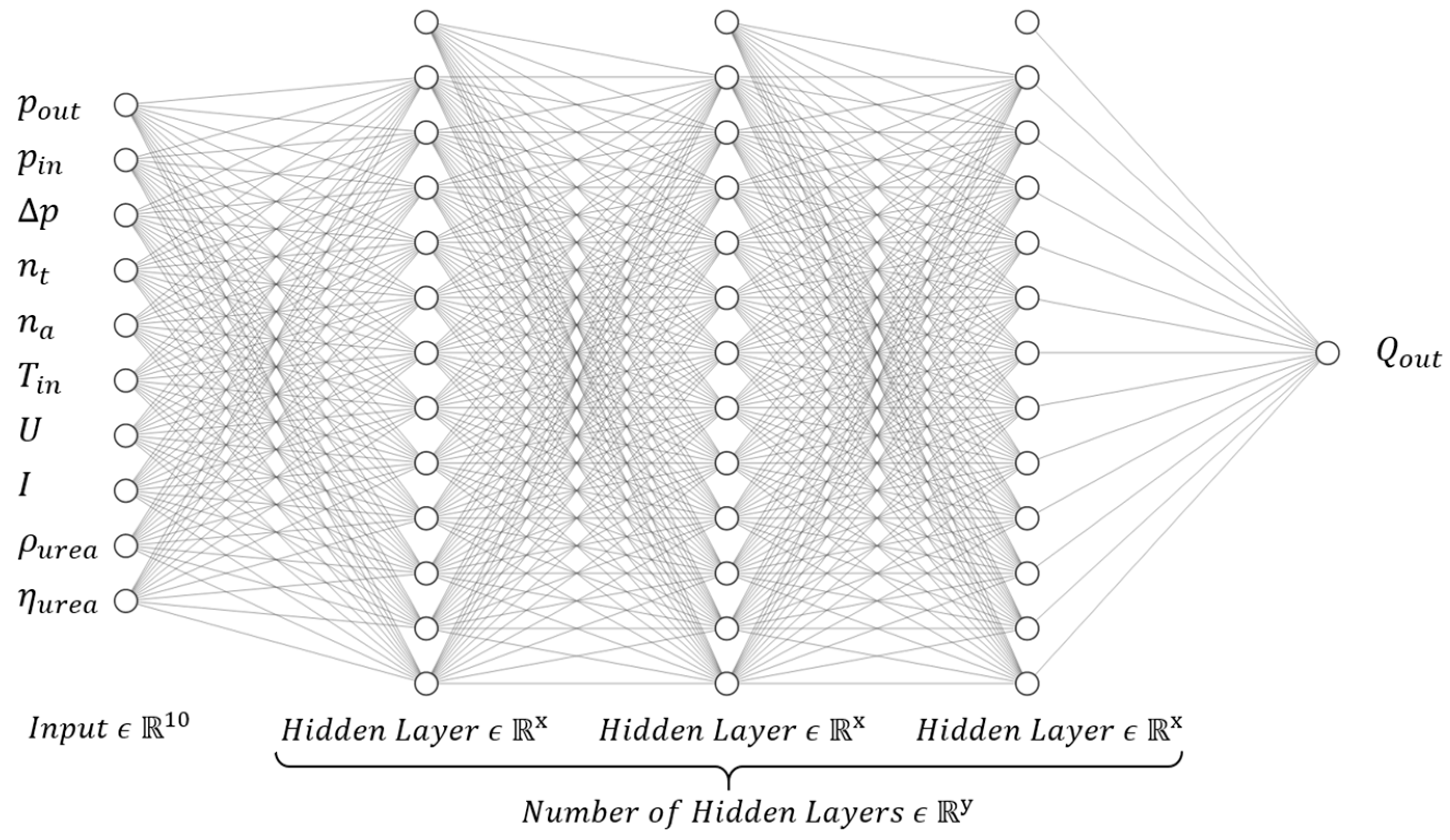
3.1. The Structure and Architecture of the Trained Neural Networks

The programmed networks are based on the TensorFlow 2.14.0 library and were created using the Python programming language. The architecture of the fast-forward neural networks is chosen as follows.

As visualized in Figure 6, all operating parameters of the entire energy chain can be fed into the neural network. Only the torque on the drive gear is not included as an input parameter for this application, as the test rig does not provide this measured variable. The number of perceptrons is fixed to the value $x$, which must be determined as part of a hyperparameter study. All hidden layers simply have the same number of perceptrons in our analysis. Furthermore, the number $y$ of hidden layers must be determined. The aim is to check how small the neural network can be in the application while still being able to predict the volumetric flow $Q_{out}$ of the pump properly. Since computing power is a limited resource on microcontrollers, where the neural network shall be operated later, such neural networks must be sparse and small, so that they can actually be placed into the application.

The hyperbolic tangent (tanh) activation function is chosen, as we expect a smoother interpolation of the characteristic pump curve.

$$tanh(x)=\frac{e^x-e^{-x}}{e^x+e^{-x}}$$

(10)

In our considerations, the neural network receives only one type of activation function. We do not mix activation functions within the hidden layers because we want to keep the network structure as simple as possible. The input variables are normalized using the standard normalizer from the scikit-learn library to improve the regression of the neural network. The input variables are normalized for each input individually using the mean value and the standard deviation of the training dataset.

The mean squared error (MSE), which is one of the most commonly used functions for neural networks, is used to calculate the error within the adaptive moment estimation (Adam) backpropagation training algorithm. We add L1 regularization with a regularization parameter $\lambda =0.001$ for each hidden layer to counteract overfitting of the weight vectors ${\theta }_j$ within the set of trainable parameters $k$ [36].

$$Loss\left(\theta \right)=\frac{1}{m}\sum _{i=1}^m{(Y_i-{\widehat{Y}}_i)}^2+\frac{\lambda }{m}\sum _{j=1}^k\left|{\theta }_j\right|$$

(11)

The mean absolute percentage error (MAPE) is primarily used as a metric. As this specific error function reacts more sensitive to very small values, the mean absolute error (MAE) is also specified as a metric.

$$MAE=\frac{1}{m}\sum _{i=1}^m\left|Y_i-{\widehat{Y}}_i\right|$$

(12)

The control of the electrical motor driving the gear pump is based on an open or closed loop. Depending on the type of control, the voltage and current are not available at all rotational frequencies, as these parameters can be fixed to a specific value depending on the underlying control system architecture. We therefore recommend case differentiation as per

Table 2. Case differentiation: inputs used for neural networks.

Scenario/Use Case	Input Parameters
Approximation of the volumetric flow rate based on the whole energetic chain	$p_{out}$—outlet pressure $p_{in}$—inlet pressure $\Delta p$—pressure difference over the inlet and outlet $n_t$—target rotational frequency $n_a$—actual rotational frequency $T_{in}$—inlet Temperature $U$—electrical voltage $I$—electrical current ${\rho }_u$—density of urea–water solution ${\eta }_u$—dynamic viscosity of urea–water solution
Approximation of the volumetric flow rate based on the hydraulic domain	$p_{out}$—outlet pressure $p_{in}$—inlet pressure $\Delta p$—pressure difference over the inlet and outlet $n_t$—target rotational frequency $n_a$—actual rotational frequency $T_{in}$—inlet temperature

.

We can determine the relationships and relevant input parameters by comparing the networks. Furthermore, the second use case has another advantage. The interpolated pump characteristic curve can be easily visualized with this model variant, as the input parameters are unrelated.

Typically, neural networks are considered black-box models, which provide users with little or no insight into the mode of action. However, this variant makes it possible to visualize the regression of the pump characteristic curve over the relevant operating range. This means that we can plot the regression and easily validate the results from a human perspective.

3.2. Key Features of the Dataset

The specifications of the pumps being used limit the range of the chosen input parameters. The maximum differential pressure does not exceed 9 bar, as the technical specification of the used pumps suggests. The rotation frequency spectrum covers a range of about 200 to 4000 rotations per minute. A temperature range of 5–50 °C is selected as this easily exceeds the typical operation range of the underlying conceived industrial application. The low volumetric flow does not exceed a value of 10 mL/min. A total of six pumps from one production lot are used to demonstrate the functionality of the network architectures. The pumps all have different gap dimensions, leading to heavily varying pump characteristics within the same series. Within an applicational scenario, the pump always works against the hydraulic resistance of the system. Therefore, accurate estimation of the theoretical volume flow $Q_{theo}$ is only possible at low rotational frequencies. We take care to include more than 10 operating points for each pump curve so that the network learns to approximate the curve correctly. Therefore, at least 10 different valve positions are approached per pump curve.

To validate the network, we divide the dataset into 80% for training and 20% for testing with a random seed per pump. The neural network should learn to interpolate the pump characteristic curves. Consequently, the training of the neural network only succeeds if the pump curve fields are interpolated over the entire operating range of the pumps. For this reason, we ensure that the testing dataset contains pump curves that are not present in the training dataset. Therefore, the dataset contains operational points which are not included in the training dataset. This approach makes it possible to differentiate the datasets significantly from each other and thus to fully test the functionality of the neural networks. A total of 15,333 operating points were measured for all 6 pumps.

4. Results

This chapter is divided into several sections, which contain polynomial regressions, the hyperparameter study, the validation of the neural networks and the cross-validation across the used pumps.

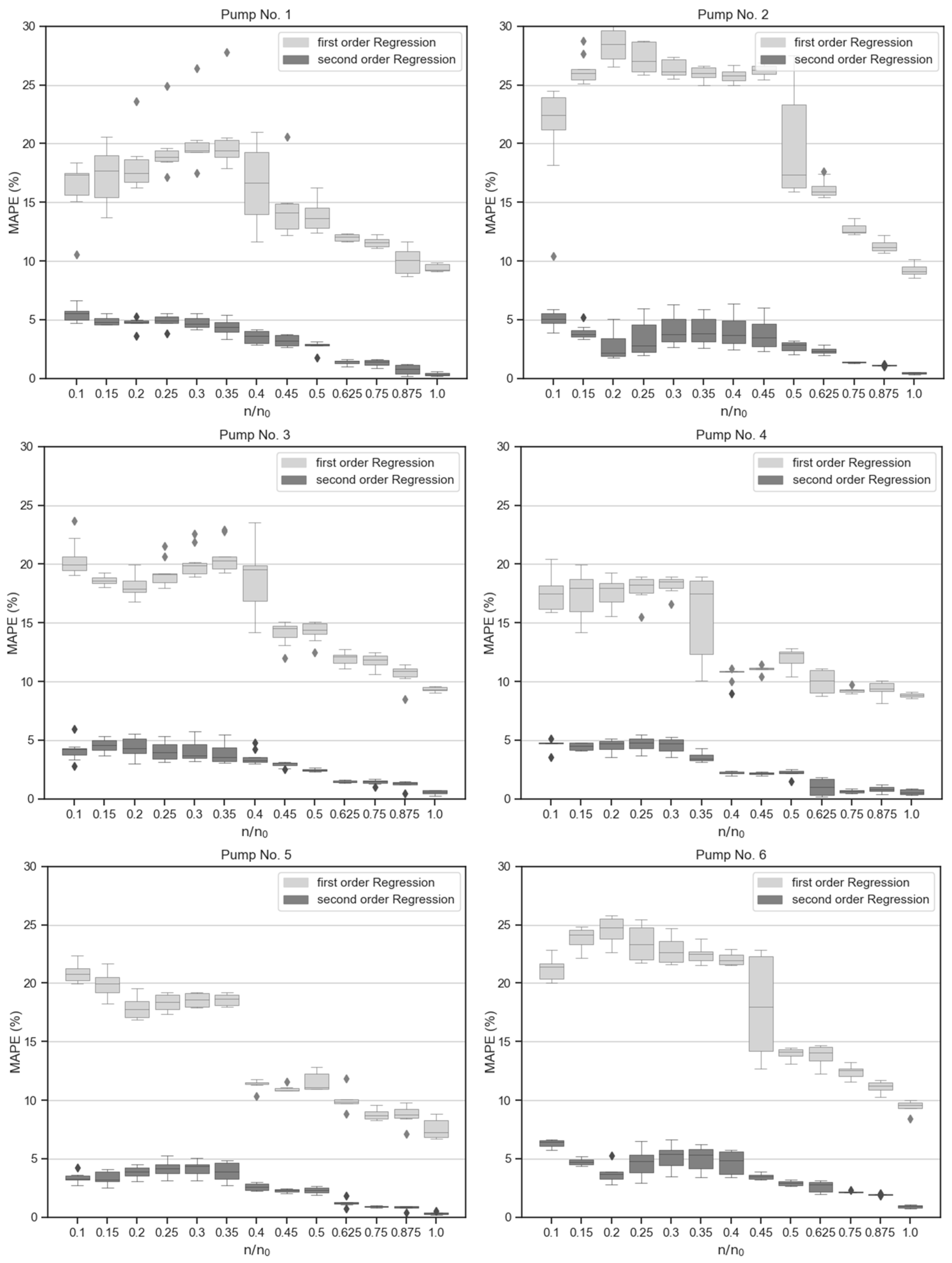
4.1. Benchmarking: First- and Second-Order Polynomial Regression

The presented model is based on our new generated dataset. For this reason, the first section contains the results of conventional polynomial regressions. The linear regression reflects the lumped parameter model, as the volume flow $Q_{out}$ is proportional to the differential pressure $\Delta p$ at a given rotational frequency $n$. The hydraulic resistance $R_{hyd}$ is therefore determined for each individual pump characteristic curve using a linear regression.

$$Q_{out}(\Delta p)=Q_{theo}-\frac{\Delta p}{R_{hyd}}=V_{theo}\cdot n-\frac{\Delta p}{R_{hyd}}$$

(13)

The second-degree polynomial regression represents the flow characteristics of complex pipe networks, which reflect turbulent and laminar flow components. The quadratic formula for the pressure formation in complex pipe networks forms the basis for this approach. However, the target variable (volumetric flow) must represent a function of the input variable (differential pressure). Therefore, the quadratic formula is solved analytically:

$$Q_{out}(\Delta p)=Q_{theo}-\left(\frac{-{\zeta }_{lam}\pm \sqrt{{{\zeta }_{lam}}^2-4\cdot {\zeta }_{turb}\cdot (-\Delta p)}}{2\cdot {\zeta }_{turb}}\right)$$

(14)

The presented regression variants fit the pump characteristic curves individually. This benchmark approach does not represent a multidimensional regression task. We fit the individual pump characteristics of the rotational frequencies and temperatures separately within this benchmark test. A multidimensional regression model, as the neural network consequently represents, can only be created when the hyperparameters of the regressions, i.e., the hydraulic resistance $R_{hyd}$ and the parameters of the quadradic term ${\zeta }_{lam}$ and ${\zeta }_{turb}$, are interpolated over the rotational frequencies and temperatures.

This benchmark approach only intends to enable a comparison. The neural network, however, learns to approximate the pump characteristics field over the entire range of rotational frequencies and temperatures (See

Table 3. Validation of the first- and second-order polynomial regression.

Pump	MAPE (%)		MAE (mL/min)
	First Order	Second Order	First Order	Second Order
1	15.44	3.27	51.36	9.68
2	21.29	3.01	53.92	8.92
3	16.00	2.99	52.29	9.76
4	13.50	2.85	48.15	8.88
5	14.09	2.56	44.89	8.28
6	18.41	3.72	53.85	12.39
Total Average	16.46	3.07	50.74	9.65

).

In total, the first- and second-order regressions achieve a total MAPE of 16.46% and 3.07%. The second-order regressions achieve the same accuracy as the cited CFD simulations indicate, as the volumetric vortices are also taken into account in this approach. Appendix A contains the exact analysis of the MAPE and MAE over the rotational frequencies as a boxplot diagram for all six pumps.

4.2. Hyperparameter Study: Finding the Right Neural Architecture

The results of conventional regression show that it makes perfect sense to solve the regression task using neuronal networks. However, the following questions arise. Which network size should be selected, how much can the network be reduced in size, and does an enlargement of the architecture benefit the regression? For this reason, the hyperparameter study incrementally increases the number $x$ of perceptrons and the number $y$ of hidden layers. The networks are trained over 2000 epochs. The whole energetic chain is used for the approximation of the volumetric flow rate. No early stopping is applied. The following Figure 7 contains only the end results of the training process.

Even neuronal networks with six neurons produce better results than the conventional regression variants. In principle, networks with more neurons per layer achieve better results, regardless of the number of hidden layers. However, the architectures converge at an MAPE of about 0.8–1%. This result corresponds to the accuracy of the dataset, as the sensors in use have an accuracy of 0.5–1.0% Appendix B contains the hyperparameter studies of the other five pumps. These show very similar results.

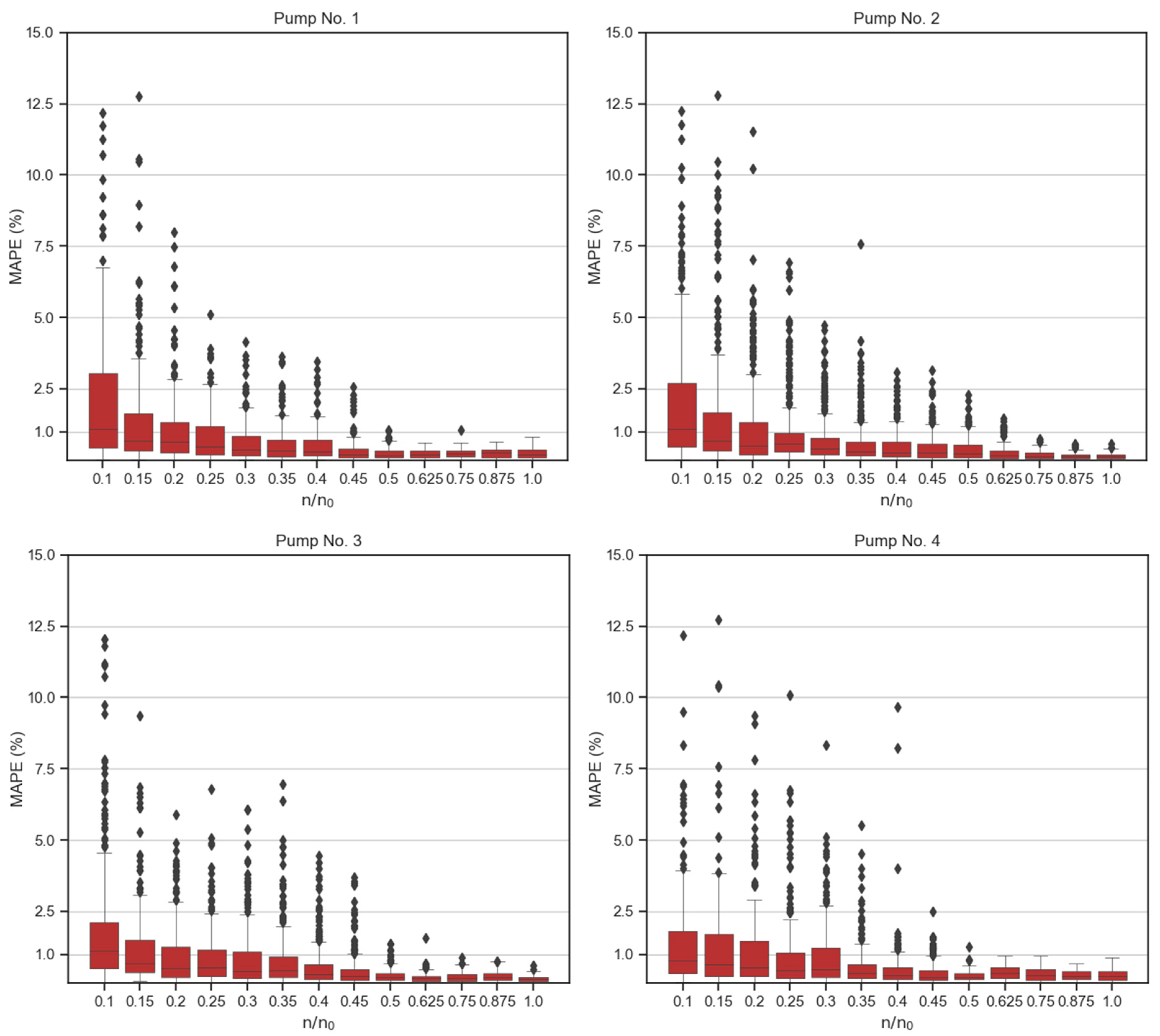
4.3. Evaluation of the Neural Network

We choose an ideal network size of 64 perceptrons with six hidden layers each for further processes, even though we could use a smaller network. This architecture corresponds to a total number of 21,569 trainable parameters, which nevertheless corresponds to a very small network in the domain of machine learning. The validation of the network over the entire training epochs can be seen in Figure 8.

The results of the test dataset do not differ significantly from those of the training dataset. This shows that the neural network does indeed learn to interpolate the pump characteristics correctly and that no overfitting occurs. The neural network eventually has almost the same accuracy of the sensors used to collect the dataset. It should be noted that the network shows a fluctuation of approximately ±1% over the entire training. Again, this error can be explained by the accuracy of the underlying dataset.

Because of the different control loops mentioned above, it is necessary to check whether the network can also predict the behavior of the pump based on the differential pressure alone.

Table 4. Case differentiation: validation of the best results of the test dataset over the epochs.

Pump	MAPE (%)		MAE (mL/min)
	Use Case 1	Use Case 2	Use Case 1	Use Case 2
1	0.83	0.97	1.31	1.56
2	0.93	0.96	1.11	1.12
3	0.83	0.86	1.21	1.22
4	0.93	0.96	1.57	1.61
5	0.75	0.70	1.09	1.17
6	0.82	0.77	1.31	1.16
Total Average	0.85	0.87	1.27	1.31

Use case 1—approximation of the volumetric flow rate based on the whole energetic chain, use case 2—approximation of the volumetric flow rate based on the hydraulic domain.

compares the two scenarios in a summarized form.

The neural networks can already predict the behavior of the pumps very well based on the rotational frequency, temperature, and differential pressure alone. Although there is a known correlation between the electrical current and the volumetric flow rate in the control of the pumps, the results show that it is not necessary to include the electrical current or voltage in the algorithm.

The visualization of the approximation from the trained neural network provides valid insights. Figure 9a shows the characteristic curve field of pump 1 at a temperature of 20 °C. The dotted black lines represent the predicted pump curves where no operating points were measured. Notice the extreme points at the edges of the axes. The network appears to have approximation problems here.

The theoretical flow rates, which represent the intersection points with the x-axis, are not optimally approximated at higher rotational frequencies. However, this error is negligible, as the pump can never reach the theoretical volume flow at higher rotational frequencies, as the inflows and outflows of the pump alone create hydraulic resistance. At higher rotational frequencies, the neural network does not succeed in accurately mapping the pump curve. The distance between the pump characteristics is formed via the rotational frequency $n$. The difference $\Delta n$ is too large, which is why the network has difficulties. The operating points are not optimally selected either, which results in fluctuating and wavy approximated pump curves.

A further conspicuous feature occurs at the extreme points on the y-axis. The maximum differential pressure of the pump is not reproduced correctly either. As the dataset contains operating points of $Q>10 \mathrm{m}\mathrm{L}∕\mathrm{m}\mathrm{i}\mathrm{n}$, the neural network is also only valid for this range. In particular, the temperature deviations shown in Figure 9b, which include the changes in the leakage gap and the changes in the material properties, appear to be correctly mapped by the network. Appendix C contains the pump curve fields of the other remaining pumps.

Figure 10 compares the conventional regression variants and the results of the trained neural network. The MAPE and MAE are displayed over the entire rotational frequency range. The varying differential pressures and the temperature spectrum cause the scatter within the box-plot diagram. At low rotational frequencies, the network appears to have more outliers, which are visualized as black dots within the box plot. These specific outliers are very small volume flow values, which stand out in particular due to the metric of the percentage error. The superiority of the neural network becomes extremely clear with higher rotational frequencies in particular.

Appendix D contains the visualization of the MAPE and the MAE over the rotational frequencies for the remaining pumps.

Although the results show that neural networks are suitable for modeling the behavior of pumps, there are still some weaknesses in this approach. It is indeed possible to map the characteristic curve fields of the pumps. However, an individual dataset is required for each pump because the neural architectures used are difficult to transfer due to mechanical tolerances of the manufactured pumps. The following cross-validation makes this instance clear within

Table 5. Cross-validation: validation of the neural network using multiple pump datasets.

Validation on Pump	Dataset	MAPE (%)		MAE (mL/min)
		Training	Testing	Training	Testing
1	2, 3, 4, 5, 6	2.24	10.91	2.64	12.69
2	1, 3, 4, 5, 6	1.71	37.33	2.56	34.69
3	1, 2, 4, 5, 6	1.89	9.46	2.12	14.59
4	1, 2, 3, 5, 6	3.73	15.95	3.08	27.45
5	1, 2, 3, 4, 6	2.44	9.24	2.83	13.02
6	1, 2, 3, 4, 5	2.41	2.59	19.01	25.58

Training dataset contains the operation points of five pumps; testing dataset contains the remaining pump to validate the regression task for new unknown pumps.

. Here, a meta-network is first trained with the data from five test pumps and is then validated using the remaining sixth pump. The architecture of the network remains the same with six hidden layers and 64 perceptrons for each layer. The validation method makes it possible to verify whether the network learns to interpolate between the pump characteristics.

The previous accuracy cannot be achieved within this experiment. This circumstance is not surprising, as the neural network does not receive any information about the variations of the gap geometries within the pumps. Therefore, the neural network does not receive any knowledge about how it must interpolate between the pump characteristic curves.

5. Conclusions

In this study, we introduce an alternative data-driven model based on neural networks to precisely predict the behavior of the used external gear pumps. The presented methods include the entire rotational frequency range, a large temperature spectrum, and various hydraulic resistances. Based on the presented results, the following conclusions were drawn.

• The differential pressure from the suction to the delivery side of the pump, the rotational frequency, and the fluid temperature alone make it possible to predict the flow rate of the used external geared pumps. Adding the measurements of the current and voltage as input to the neural network shows only negligible improvements in the accuracy of the network, as it already produces very precise predictions based on the differential pressure, temperature and rotational frequencies.
• Even neural networks with just six perceptrons are more accurate than conventional physically based regression variants. Very sparse neural networks with only a few hidden layers can generate an average flow rate accuracy of less than 1%.
• The accuracy of the sensors limits the quality of the regression. The neural networks are not more accurate than the underlying dataset dictates.
• As soon as the pump characteristic curves within the dataset are too far apart, i.e., the rotational frequencies of the pumps are too far apart within the dataset, the neural network has difficulties in generalizing the pump characteristic curves. These instabilities only get noticeable at higher rotational frequencies within the presented approach.

6. Discussion

The networks are difficult to use in the context of a transfer task. This result confirms the common impression of neuronal networks, as meta-learning is still a well-recognized research field. The accuracy suffers when the behavior of several pumps is approximated simultaneously, as the neural networks have no understanding of the gap geometries and cannot distinguish well between the pumps. This fact is probably reinforced when different pump types and varying fluid systems are taken into account. Since this study solves an industrial production problem, the impact of this circumstance on the scalability of the solution must be highlighted. However, this circumstance does not limit the architecture of our presented approach itself, but rather points to the need for the acquisition of new data in case of scalability to new pump designs. It is therefore primarily of economic relevance for the users. It is precisely this circumstance that generates further research interest and indicates possible potential for further studies.

The first optimization option is to investigate the extent to which it is possible to generate the same results using fewer data points. Furthermore, the transferability of the network across different production tolerances must be analyzed. However, it should be noted that the effects of different manufacturing tolerances are very significant in the case of the used external gear pump presented here, as the used pumps have very small gaps. In the case of other pump systems, whether the presented approach is still valid and whether the neural networks make equally good predictions in these cases must be checked. The chosen approach allows users to visualize the regression of the networks and to get a good understanding of the approximation. This circumstance is rather rare in the field of neural networks and therefore worth mentioning. Finally, varying pump designs and several fluid systems must be included within further studies to analyze and overcome challenges. Combining conventional modeling approaches with the presented data-driven model represents another promising field of interest for further research.

References

1. Mao, Z.; Peng, Y.; Hu, C.; Ding, R.; Yamada, Y.; Maeda, S. Soft computing-based predictive modeling of flexible electrohydrodynamic pumps. Biomim. Intell. Robot. 2023, 3, 100114. [Google Scholar] [CrossRef]
2. Ma, L.; Meng, Q.; Pan, S.; Liebman, A. PUMPNET: A deep learning approach to pump operation detection. Energy Inform. 2021, 4, 1. [Google Scholar] [CrossRef]
3. Ma, H.; Gaisser, L.; Riedelbauch, S. Monitoring Pumping Units by Convolutional Neural Networks for Operating Point Estimations. Energies 2023, 6, 4392. [Google Scholar] [CrossRef]
4. Wang, W.; Pei, J.; Yuan, S.; Gan, X.; Tingyun, Y. Artificial neural network for the performance improvement of a centrifugal pump. IOP Conf. Ser. Earth Environ. Sci. 2019, 240, 032024. [Google Scholar] [CrossRef]
5. VDMA Pumpen + Systeme VDMA Kompressoren, Druckluft- und Vakuumtechnik. Pumpen und Kompressoren für den Weltmarkt 2020 mit Druckluft- und Vakuumtechnik; VDMA Verlag GmbH: Frankfurt am Main, France; Available online: https://vdma-verlag.com/home/pumps-and-compressors_DE.html#modal-cookiewarning (accessed on 30 October 2023).
6. Bauer, G.; Niebergall, M. Ölhydraulik: Grundlagen, Bauelemente, Anwendungen, 12th ed.; Springer Fachmedien Wiesbaden GmbH: Wiesbaden, Germany, 2019; pp. 83–100. [Google Scholar]
7. Rapp, C. Hydraulik für Ingenieure und Naturwissenschaftler: Ein Kurs mit Experimenten und Open-Source Codes, 2nd ed.; Springer Fachmedien Wiesbaden GmbH: Wiesbaden, Germany, 2021; pp. 165–172. [Google Scholar]
8. DIN ISO 4391; Hydraulic Fluid Power; Pumps, Motors and Integral Transmissions; Parameter Definitions and Letter Symbols. ISO: Geneva, Switzerland, 1994.
9. DIN ISO 4409; Hydraulic Fluid Power—Positive-Displacement Pumps, Motors and Integral Transmissions—Methods of Testing and Presenting Basic Steady State Performance. ISO: Geneva, Switzerland, 2019.
10. Antoniak, P.; Stryczek, J. Visualization study of the flow processes and phenomena in the external gear pump. Arch. Civ. Mech. Eng. 2018, 18, 1103–1115. [Google Scholar] [CrossRef]
11. Huang, K.J.; Lian, W.C. Kinematic flowrate characteristics of external spur gear pumps using an exact closed solution. Mech. Mach. Theory 2009, 44, 1121–1131. [Google Scholar] [CrossRef]
12. Zhao, X.; Vacca, A. Theoretical Investigation into the Ripple Source of External Gear Pumps. Energies 2019, 12, 535. [Google Scholar] [CrossRef]
13. Vacca, A.; Devendran, R.S. Theoretical analysis for variable delivery flow external gear machines based on asymmetric gears. Mech. Mach. Theory 2017, 108, 123–141. [Google Scholar] [CrossRef]
14. Tian, H. Dynamic Pressure Simulation of an External Gear Pump with Relief Chamber Using a Morphological Approach. IEEE Access 2018, 6, 77509–77518. [Google Scholar] [CrossRef]
15. Wilhelmsmeyer, T. Zahnradpumpen in der Elastomertechnik. Ph.D. Thesis, Faculty of Mechanical Engineering (University Paderborn), Paderborn, Germany, 16 February 2006. [Google Scholar]
16. ISO 4359; Flow Measurement Structures Rectangular, Trapezoidal and U-Shaped Flumes. ISO: Geneva, Switzerland, 2022.
17. Mucchi, E.; DÈlia, G.; Dalpiaz, G. Simulation of the running in process in external gear pumps and experimental verification. Meccanica 2012, 47, 621–637. [Google Scholar] [CrossRef]
18. Rundo, M. Models for Flow Rate Simulation in Gear Pumps: A Review. Energies 2017, 10, 1261. [Google Scholar] [CrossRef]
19. Zhou, J.; Vacca, A.; Casoli, P. A novel approach for predicting the operation of external gear pumps under cavitating conditions. Simul. Model. Pract. Theory 2014, 45, 35–49. [Google Scholar] [CrossRef]
20. Marinaro, G.; Frosina, E.; Senatore, A. A Numerical Analysis of an Innovative Flow Ripple Reduction Method for External Gear Pumps. Energies 2021, 14, 471. [Google Scholar] [CrossRef]
21. Vacca, A.; Guidetti, M. Modelling and experimental validation of external spur gear machines for fluid power applications. Simul. Model. Pract. Theory 2011, 19, 2007–2031. [Google Scholar] [CrossRef]
22. Torrent, M.; Gamez-Montero, P.J.; Codina, E. Parameterization, Modeling, and Validation in Real Conditions of an External Gear Pump. Sustainability 2021, 13, 3089. [Google Scholar] [CrossRef]
23. Engler, M. Simulation, Design and Analytical Modelling of Passive Convective Micromixers for Chemical Production Purposes; Shaker Verlag: Aachen, Germany, 2006; p. 22. ISBN 3-8322-5130-1. [Google Scholar]
24. Torrent, M.; Gamez-Montero, P.J.; Codina, E. Motion Modelling of the Floating Bushing in an External Gear Pump Using Dimensional Analysis. Actuators 2023, 12, 338. [Google Scholar] [CrossRef]
25. Mucchi, E.; Dalpiaz, G.; Fernàndez del Rincòn, A. Elastodynamic analysis of a gear pump. Part I: Pressure distribution and gear eccentricity. Mech. Syst. Signal Process. 2010, 24, 2160–2179. [Google Scholar] [CrossRef]
26. Mucchi, E.; Dalpiaz, G.; Rivola, A. Elastodynamic analysis of a gear pump. Part II: Meshing phenomena and simulation results. Mech. Syst. Signal Process. 2010, 24, 2180–2197. [Google Scholar] [CrossRef]
27. Zardin, B.; Natali, E.; Borghi, M. Evaluation of the Hydro—Mechanical Efficiency of External Gear Pumps. Energies 2019, 12, 2468. [Google Scholar] [CrossRef]
28. Shorr, B. Thermal Integrity on Mechanics and Engineering; Springer: Berlin, Germany, 2015. [Google Scholar] [CrossRef]
29. Frosina, E.; Senatore, A.; Rigosi, M. Study of a High-Pressure External Gear Pump with a Computational Fluid Dynamic Modeling Approach. Energies 2017, 10, 1113. [Google Scholar] [CrossRef]
30. Szwemin, P.; Fiebig, W. The Influence of Radial and Axial Gaps on Volumetric Efficiency of External Gear Pumps. Energies 2021, 14, 4468. [Google Scholar] [CrossRef]
31. Corvaglia, A.; Rundo, M.; Casoli, P.; Lettini, A. Evaluation of Tooth Space Pressure and Incomplete Filling in External Gear Pumps by Means of Three-Dimensional CFD Simulations. Energies 2021, 14, 342. [Google Scholar] [CrossRef]
32. Yoon, Y.; Park, B.H.; Shim, J.; Han, Y.O.; Hong, B.J.; Yun, S.H. Numerical simulation of three-dimensional external gear pump using immersed solid method. Appl. Therm. Eng. 2017, 118, 539–550. [Google Scholar] [CrossRef]
33. Halonen, S.; Kangas, T.; Haataja, M. Urea-Water-Solution Properties: Density, Viscosity, and Surface Tension in an Under-Saturated Solution. Emiss. Control Sci. Technol. 2016, 3, 161–170. [Google Scholar] [CrossRef]
34. Haynes, W.M.; Lide, D.R.; Bruno, T.J. CRC Handbook of Chemistry and Physics: A Ready-Reference Book of Chemical and Physical Data, 95th ed.; CRC Press Taylor & Francis Group: Baca Raton, FL, USA, 2014; pp. 6–7. [Google Scholar]
35. Kurt, H.; Maxwell, S. Multilayer Feedforward Networks are Universal Approximators. Neural Netw. 1989, 2, 359–366. Available online: https://cognitivemedium.com/magic_paper/assets/Hornik.pdf (accessed on 30 November 2023).
36. TensorFlow v2.14.0. Available online: https://www.tensorflow.org/api_docs/python/tf/keras/regularizers/L1 (accessed on 15 November 2023).
Figure 1. Operating principle and system flow of an external gear pumps.
Processes 12 00526 g001
Figure 2. Energetic chain of effects for the external pumps in use. I —electrical current, U —electrical voltage, P e l —electrical power, η e l , m e c h —electrical–mechanical degree of efficiency, P m e c h —mechanical power, M —moment, n —rotation frequency, η m e c h ,   h y d —mechanical–hydraulic degree of efficiency, P h y d —hydraulic power, p e f f —effectively usable pressure, Q e f f —effectively usable volume flow, Q l o s s —leakage losses.
Processes 12 00526 g002
Figure 3. Breakdown of leakage losses within the external gear pump. Q f a c e —volumetric loss over the face of tooth, Q h e a d —volumetric loss within head gap, Q b e a r i n g —volumetric loss within bearings, Q m e s h i n g —volumetric loss due to meshing, h h e a d —head gap height, h f a c e —face gap height, d h e a d —tooth head diameter, b t o o t h —tooth width.
Processes 12 00526 g003
Figure 4. Test setup with (a) systematic drawing of the hydraulic circuit; (b) 3D CAD visualization of the test field.
Processes 12 00526 g004
Figure 5. (a) Temperature-dependent density of urea in comparison to water; (b) temperature-dependent viscosity of urea in comparison to water.
Processes 12 00526 g005
Figure 6. Visualization of the fast-forward neural network architecture. p o u t —outlet pressure, p i n —inlet pressure, Δ p —pressure difference over the inlet and outlet, n t —target rotational frequency, n a —actual rotational frequency, T i n —inlet temperature, U —electrical voltage, I —electrical current, ρ u —density of urea–water solution, η u —dynamic viscosity of urea–water solution, x —number of perceptrons per hidden layer, y —number of hidden layers.
Processes 12 00526 g006
Figure 7. (a) Validation of MAPE for pump 1; (b) Validation of MAE for pump 1.
Processes 12 00526 g007
Figure 8. (a) Validation of MSE loss over all epochs; (b) validation of MAPE metric over all epochs; (c) validation of MAE loss over all epochs.
Processes 12 00526 g008
Figure 9. (a) Visualization of the prediction from the neural network at T = 20 °C; (b) visualization of temperature effects on the pump curve approximation.
Processes 12 00526 g009
Figure 10. (a) Visualization of the MAPE over the rotational frequencies; (b) visualization of the MAE over the rotational frequencies.
Processes 12 00526 g010