Prediction of Energy Consumption in a Coal-Fired Boiler Based on MIV-ISAO-LSSVM

Abstract

Aiming at the problem that the energy consumption of the boiler system varies greatly under the flexible peaking requirements of coal-fired units, an energy consumption prediction model for the boiler system is established based on a Least-Squares Support Vector Machine (LSSVM). First, the Mean Impact Value (MIV) algorithm is used to simplify the input characteristics of the model and determine the key operating parameters that affect energy consumption. Secondly, the Snow Ablation Optimizer (SAO) with tent map, adaptive t-distribution, and the opposites learning mechanism is introduced to determine the parameters in the prediction model. On this basis, based on the operation data of an ultra-supercritical coal-fired unit in Xinjiang, China, the boiler energy consumption dataset under variable load is established based on the theory of fuel specific consumption. The proposed prediction model is used to predict and analyze the boiler energy consumption, and a comparison is made with other common prediction methods. The results show that compared with the LSSVM, BP, and ELM prediction models, the average Relative Root Mean Squared Errors (aRRMSE) of the LSSVM model using ISAO are reduced by 2.13%, 18.12%, and 40.3%, respectively. The prediction model established in this paper has good accuracy. It can predict the energy consumption distribution of the boiler system of the ultra-supercritical coal-fired unit under variable load more accurately.

1. Introduction

The combination of practical engineering problems with data analysis and mechanism interpretation has become increasingly popular with the rapid development of big data analysis technology and intelligent machine learning algorithms [1,2]. In this context, historical operation data of coal-fired units is particularly important for optimizing unit operation and diagnosing unit status. Simple mechanism analysis can be misleading due to experience, hence the need for a more comprehensive approach. Many researchers are now focusing on the intersection of mechanism analysis, data mining, machine learning, and other related disciplines. The operation, control, design, and transformation of the unit are studied using extensive historical data.

Currently, numerous scholars have utilized machine learning and data mining techniques in researching thermal power units. Yang et al. [3] proposed a soft-sensor model for NO_X concentration at the SCR outlet based on the gated cyclic unit neural network. Yang et al. [4] conducted a study on the optimization of the collaborative recovery system of flue gas waste heat and water in coal-fired units. Sun et al. [5] established an NO_X prediction model for coal-fired units using Bayesian optimization combined with random forest, providing assistance for NO_X emission control. Dai et al. [6] proposed a hierarchical clustering retrieval strategy based on the fuzzy C-means clustering algorithm to construct an offline database; they also employed a multi-attribute decision-making method that comprehensively considered multiple objectives to extract optimal decision samples from the database and then guide the load scheduling scheme of power plants. Blackburn et al. [7] conducted dynamic optimization for variable load control of coal-fired units using the particle swarm optimization algorithm and LSTM. Wang et al. [8] used clustering and prediction algorithms to build a multi-objective regression model to predict and control boiler efficiency, improve boiler combustion efficiency, and reduce NOx emissions.

In the study of unit energy consumption, researchers typically employ data analysis and other methods to diagnose and optimize unit operation. Fu et al. [9] utilized the fuzzy rough set attribute reduction method to reduce the main characteristic parameters that affect unit energy consumption. They then established a sensitivity analysis model for unit energy consumption using support vector machines. Cai [10] proposed an intelligent algorithm that combines a generalized neural network and average influence value to classify the factors that affect the energy consumption of units. They established an energy consumption characteristic model for large coal-fired units. Xiao et al. [11] used RapidMiner, a data mining platform, to establish a prediction model for exergic efficiency of the unit, and explored the improvement space of exergic loss based on the random simulation method, so as to obtain the best working conditions of the unit under various loads and corresponding control index parameters during actual operation. Sun. [12] obtained the nonlinear relationship between power supply coal consumption and various operation control parameters by using a random forest algorithm, and combined with a genetic algorithm, proposed the unit operation optimization strategy. Wan et al. [13] developed a neural network-based model to predict steam flow at the outlet of cogeneration boilers. Wang et al. [14] developed a hierarchical energy efficiency index system for unit economic diagnosis. They analyzed the variation characteristics of key energy consumption indicators on the boiler and turbine sides through mechanism research and actual data trends, thus helping to analyze the causes of abnormal operation.

In many previous studies, researchers mainly used data analysis and other methods to carry out unit diagnosis, operation optimization, and other aspects of the work, and the accuracy of the research model will have a great impact on the effectiveness of the work. Currently, the primary prediction models consist of the neural network and support vector machine (SVM) [15]. The Least-Squares Support Vector Machine (LSSVM) model possesses the strengths of both, including the strong generalization ability and global optimization of SVM, while avoiding the issues of overfitting in neural networks and time-consuming training in SVM [16]. However, setting the hyperparameters in the LSSVM model is often based on experience, which can lead to problems such as low efficiency and a lack of precision. To address this issue, it is necessary to use optimizers to obtain the best hyperparameters.

Since China announced the ‘30·60’ decarbonization goal, traditional coal-fired units have increasingly participated in deep peak regulation to adapt to the intermittency and volatility of new energy power generation. This has led to an increase in load adjustment frequency and range during actual production. Exergy analysis reveals that the energy consumption of the boiler, which is the part of the unit with the greatest energy loss, has also changed significantly. To help staff in comprehending the operational status of a coal-fired unit under flexible peak load balancing and to support the optimization of the boiler system’s operation, this study focuses on a 660 MW coal-fired unit as the research subject. A prediction model for the boiler system’s energy consumption and distribution is established, and a prediction analysis of the boiler’s energy consumption is conducted. The paper presents the main contributions as follows: (1) Construction of the boiler energy consumption dataset using the theory of fuel specific consumption. The mean impact value algorithm is used to extract eigenvalues, resulting in a more comprehensive model input with a stronger correlation to boiler energy consumption compared to other manual input specification methods. (2) The snow ablation algorithm was improved using tent map, adaptive t-distribution, and the opposites learning mechanism to enhance its optimization ability and speed. (3) By adjusting the model’s hyperparameters using an optimization algorithm instead of manually setting the hyperparameters, the prediction model can better align with the operation of a specific unit, resulting in improved performance.

2. Improved Snow Ablation Optimizer

2.1. Snow Ablation Optimizer

The Snow Ablation Optimizer (SAO) is a kind of meta-heuristic algorithm. The source of inspiration for it arises from the sublimation and melting behavior of snow, and it shows strong performance in comparison with other optimizers [17]. The initial population is generated using the following formula:

$$X_{i,j}=r\times \left(U{B}_j-L{B}_j\right)+L{B}_j$$

(1)

where: i = 1, 2 … N; j = 1, 2, … Dim; N is the population number; Dim is the search space dimension. UB_j and LB_j are the upper and lower limits of the j-dimensional, respectively. r is the random number between 0 and 1.

There are two strategies for the algorithm to iterate:

(1)

The exploitation phase

Instead of expanding with a highly decentralized feature in the solution space, search agents are encouraged to exploit high-quality solutions around the current best solution when the snow converts into liquid water by melting behavior. The algorithm updates the regions where the optimal solution may exist based on the distribution of the current solution. The mathematical expression for this process is as follows:

$$X_{t+1}=m\times X_b+B{M}_t\otimes \left({\theta }_1\times \left(X_b-X_t\right)+\left(1-{\theta }_1\right)\times \left(\overline{X}-X_t\right)\right)$$

(2)

where: $t$ is the number of current iterations; $X_{t+1}$ is the new individual based on $X_t$; $X_b$ is the best individual in the population obtained in the t-th iteration; $B{M}_t$ indicates a vector including random numbers on the basis of Gaussian distribution denoting the Brownian motion; $\overline{X}$ is the average of all individuals in the population; $X_t$ is the individual in the population obtained in the t-th iteration; m and ${\theta }_1$ are the algorithm parameters.

(2)

The exploration phase

In the exploration phase, after snow or liquid water are formed into water vapor by sublimation or evaporation, the water vapor moves in space without rules and explores through irregular movement. Using the randomness and irregularity of Brownian motion in the SAO algorithm makes it easier for individuals in the population to explore valuable and potential areas in the exploration process. The mathematical expression for this is as follows:

$$X_{t+1}=E_t+B{M}_t\otimes \left({\theta }_2\times \left(X_b-X_t\right)+\left(1-{\theta }_2\right)\times \left(\overline{X}-X_t\right)\right)$$

(3)

where: $E_t$ refers to the individual randomly selected between the top three individuals with fitness values in the population and $\overline{X}$; ${\theta }_2$ is an algorithm parameter.

2.2. Algorithm Improvement Strategy

The SAO algorithm has two defects. The first is that during the algorithm’s execution, the population is divided into two groups, each executing one of the two strategies mentioned above. After each iteration, an individual executing the exploitation strategy is randomly selected to switch to the exploration strategy. This means that the exploitation phase ends after $N/2$ iterations. However, this processing method may not be conducive to a comprehensive solution. Therefore, in this paper, when $t\le \left(2/3\right)T$, exploitation and exploration occur in parallel, and the number of individuals is in a 1:2 ratio, and when $t\le \left(2/3\right)T$, all individuals execute the exploration strategy. The second issue is that the original algorithm completely discards the old individual after each iteration, yet the new individual may be worse than the old one. Therefore, this paper compares the fitness of the old and new individuals, retains the better one, and improves the improved Snow Ablation Optimizer (ISAO) using the following three methods.

(1)

Tent map

The generation rule for the initial population has a significant impact on the efficiency of the intelligent optimization algorithm. A uniformly distributed population in the initial stage of the algorithm can expand the search range of the algorithm, leading to improved convergence speed and solving accuracy. To ensure a more comprehensive and balanced initial population, a tent map is used in this paper [18], which is defined as follows:

$$p_{\left(n+1\right)}=\left\{\begin{array}{l}{p}_n/\tau ,p_n\le \tau \\ \frac{\left(1-p_n\right)}{\left(1-\tau \right)} ,p_n>\tau \end{array}\right.$$

(4)

where $p_n$ and $p_{\left(n+1\right)}$ are tent sequence values from the tent map and they are used to replace r in Formula (1); τ is the threshold with a value of 0.7. The random number r used in Formula (1) is replaced by the generated tent sequence values.

(2)

Adaptive t-distribution

The adaptive t-distribution’s probability density function is given by [19]:

$$p_{\left(x\right)}=\frac{\Gamma \left(\frac{n+1}{2}\right)}{\sqrt{n\pi }\Gamma \left(\frac{n}{2}\right)}\times {\left(1+\frac{x^2}{n}\right)}^{\frac{n+1}{2}}$$

(5)

When n equals 1, $p_{\left(n\right)}\sim C\left(0,1\right)$, it is a Cauchy distribution. As n increases, the t-distribution approaches normality. When $n\to \infty$, $p_{\left(n\right)}\to N\left(0,1\right)$, it is approximate Gaussian distribution. This paper uses the adaptive t-distribution and its mutation operators $\lambda$ to update the potential regional locations of the optimal solution determined by the exploitation strategy. This improves the algorithm’s global search ability. The variable n represents the current iteration number t, and the formula for updating the position is as follows:

$${X^{\prime }}_t=X_t+\lambda p_t{X}_t$$

(6)

where: ${X^{\prime }}_t$ is the updated individual; $\lambda =1-t/\left(T-1\right)$. With the increase of the number of iterations, its effect of controlling variation becomes weaker.

(3)

Opposites learning mechanism

During the algorithm’s exploration stage, the opposites learning mechanism [20] was used to prevent local optimization. After each iteration, the optimal and worst solutions were selected, and their corresponding opposite solutions were calculated. The better solution was then retained. The opposite solution $X_t^{op}$ was obtained from the following formula:

$$X_t^{op}=\frac{LB+UB}{2}+\frac{LB+UB}{2\theta }-\frac{X_t}{\theta }$$

(7)

In this paper, $\theta =1$, and the above formula is standard opposites learning.

(4)

Quick search strategy

After implementing the aforementioned strategies, the algorithm’s optimization ability was enhanced, albeit at a slight cost to its speed. Consequently, this paper employs the following formula to update the exploration stage, with the aim of bringing the entire population closer to the optimal solution and improving the algorithm’s efficiency.

$${X_t}^{\prime }=X+r\times \left(\overline{X}-X_t\right)$$

(8)

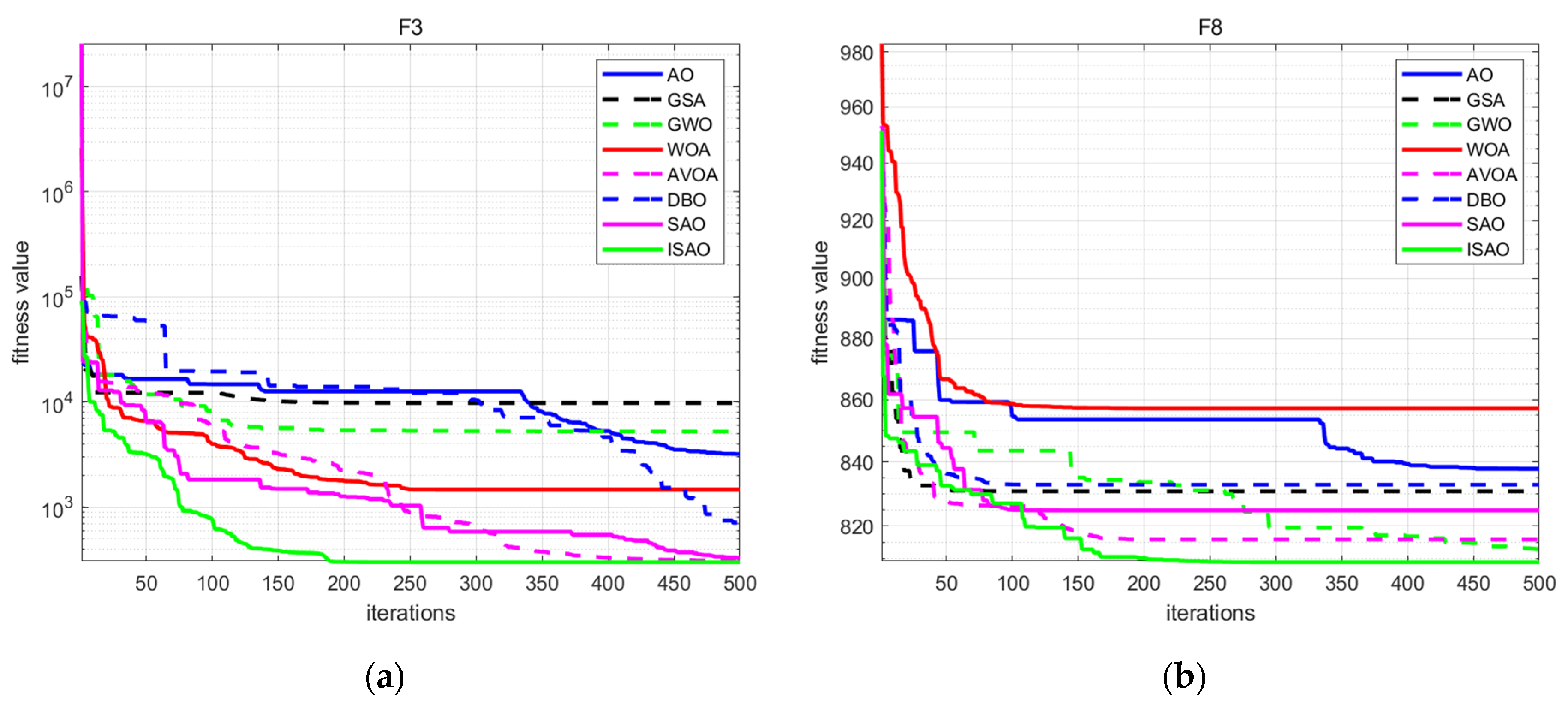
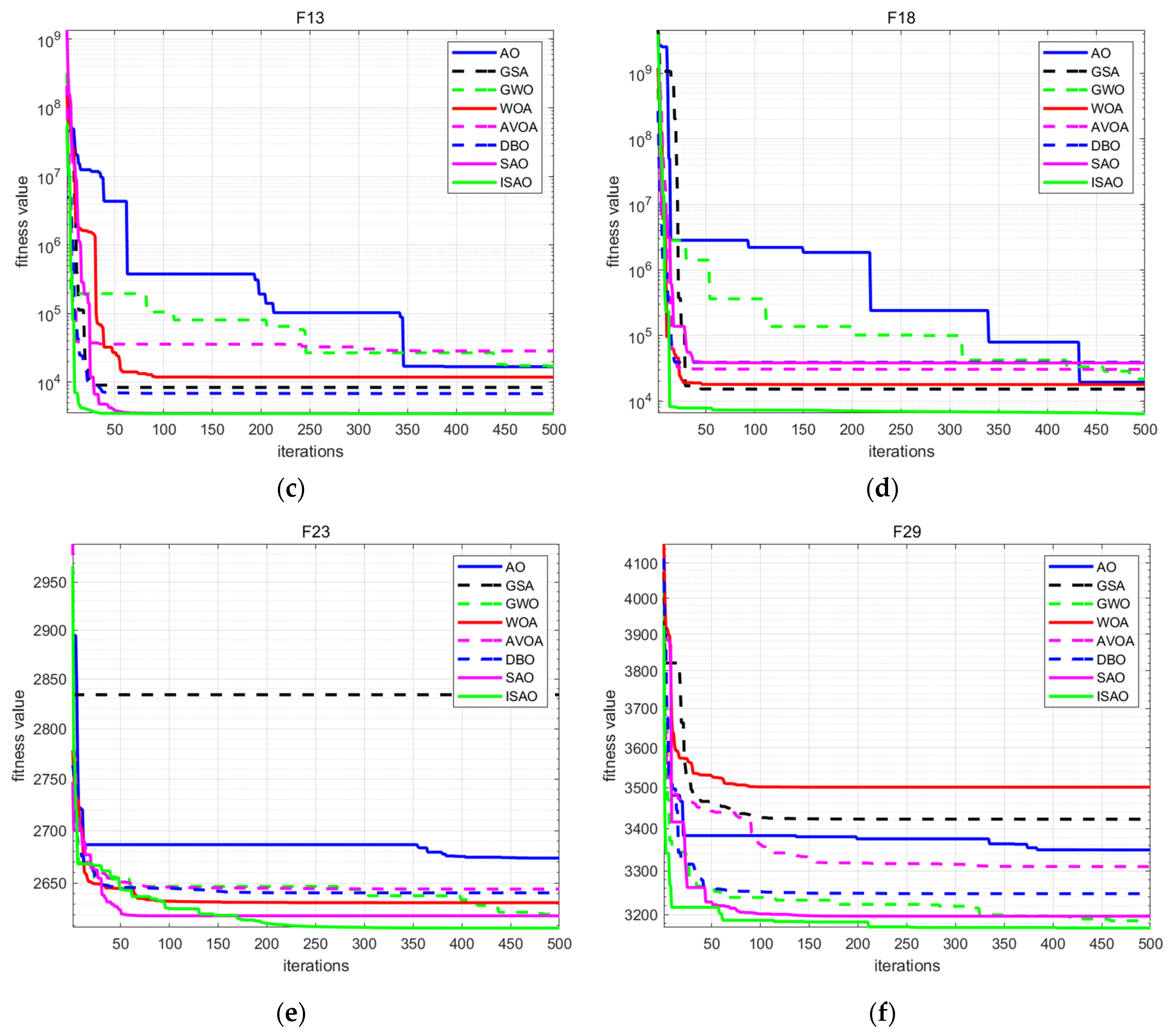
2.3. ISAO Optimization Ability Test

To test the effectiveness of ISAO, this paper selected several test functions from the CEC2017 standard function test library for optimization ability testing.

Table 1. Test functions form CEC2017.

Test Function	Dimension	Search Range	Optimal Solution
Shifted and Rotated Zakharov Function	10	[−100, 100]	300
Shifted and Rotated Non-Continuous Rastrigin’s Function	10	[−100, 100]	800
Hybrid Function 3	3	[−100, 100]	1300
Hybrid Function 6	5	[−100, 100]	1800
Composition Function 3	4	[−100, 100]	2300
Composition Function 9	3	[−100, 100]	2900

displays the expressions of the test functions and their corresponding parameters. ISAO was compared with commonly used optimizers such as AO [21], GSA [22], GWO [23], WOA [24], AVOA [25], and DBO [26]. Each function was tested 30 times, and the results were averaged.

Table 2. Comparison of different optimizers.

Test Function	Optimizers	Optimal Fitness	Optimizers	Optimal Fitness
F3	ISAO	300.000	DBO	710.895
	SAO	326.937	GSA	9790.301
	AO	3199.818	GWO	5257.905
	AVOA	309.023	WOA	1465.277
F8	ISAO	807.057	DBO	832.833
	SAO	815.919	GSA	830.844
	AO	837.849	GWO	812.931
	AVOA	815.919	WOA	857.138
F13	ISAO	3452.194	DBO	6783.287
	SAO	3492.485	GSA	8377.862
	AO	16,804.696	GWO	17,089.842
	AVOA	28,475.712	WOA	11,839.759
F18	ISAO	6365.220	DBO	38,942.046
	SAO	38,069.597	GSA	15,188.760
	AO	19,341.321	GWO	21,467.438
	AVOA	30,375.804	WOA	17,808.072
F23	ISAO	2607.639	DBO	2640.688
	SAO	2619.127	GSA	2833.831
	AO	2673.621	GWO	2620.237
	AVOA	2644.219	WOA	2631.444
F29	ISAO	3169.441	DBO	3247.289
	SAO	3196.178	GSA	3422.736
	AO	3349.266	GWO	3183.158
	AVOA	3310.118	WOA	3501.046

shows that ISAO outperforms SAO and other algorithms in multiple test functions, achieving a significantly lower optimal value and demonstrating better ability to escape local optima. Figure 1 displays the iterative graph of fitness values for different algorithms. Although the graph shows that ISAO is not the fastest of all optimizers in terms of optimization speed, it requires fewer iterations to achieve convergence compared to SAO, as seen in graphs (a), (c), and (d). In general, the ISAO algorithm has advantages in terms of convergence speed and optimization ability.

3. Boiler Energy Consumption Prediction Model

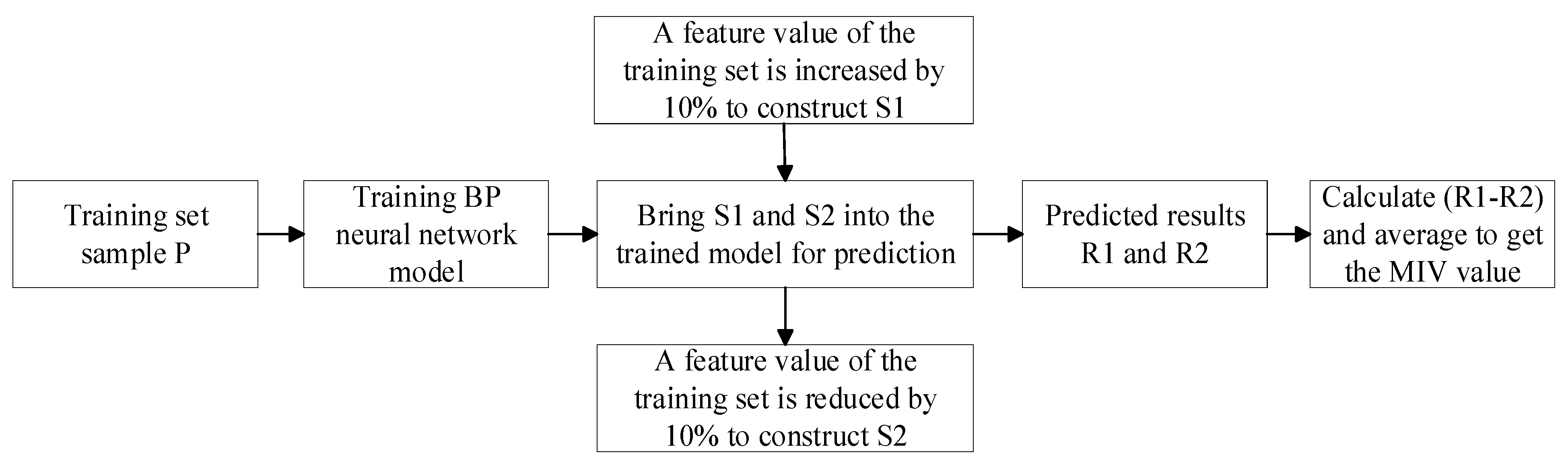
3.1. Mean Impact Value

The selection of input features has a direct impact on the accuracy and computational efficiency of the model. Currently, the Mean Impact Value (MIV) algorithm is considered one of the best methods for achieving data dimensionality reduction when combined with neural networks [27,28,29]. The MIV algorithm measures the importance of independent variables to the dependent variable by comparing the absolute value of the MIV of each feature. The positive and negative values of the variable indicate a positive or negative correlation between the independent and dependent variables, respectively.

Since the MIV algorithm needs to be combined with a neural network to realize feature screening, a back propagation neural network (BP) was selected in this paper. Firstly, a BP model was constructed using the training samples. Secondly, each feature in the training sample was increased or decreased by 10% on the original basis to form two new training samples. Finally, the BP model was used to predict and calculate the new sample data. The MIV value of the feature on the output was obtained by arithmetically averaging the difference between the two results, which reflects the influence of the feature on the output after proportional increase or decrease. Figure 2 displays the specific flow chart.

3.2. Least-Squares Support Vector Machine

Suykens et al. [30,31] developed the Least-Squares Support Vector Machine (LSSVM) by transforming the solution of the original quadratic programming problem into the solution of linear equations. The mathematical theory is presented below.

For nonlinear regression samples {x_i, y_i} (i = 1, 2, 3, …, n; x_i ∈ Rⁿ), a mapping function is introduced to map them to a high-dimensional space for linear regression. In this space, LSSVM is expressed as:

$$y={\omega }^T\phi \left(x\right)+b$$

(9)

where: ${\omega }^T$ is the weight vector; b is the offset quantity.

The function and constraints are objective and clearly stated:

$$\left\{\begin{array}{l}\min J\left(\omega ,\zeta \right)=\frac{1}{2}{\omega }^T\omega +\frac{1}{2}\gamma {\displaystyle \sum _{i=1}^n{\zeta }_i^2}\\ s.t.y_i={\omega }^T\phi \left(x_i\right)+b+{\zeta }_i\end{array}\right.$$

(10)

where: ${\zeta }_i$ is the relaxation variable; $\gamma$ is a regularization parameter.

Introducing the Lagrange multiplier α = [α₁, …, α_n], we obtain:

$$L\left(\omega ,\zeta ,b,\alpha \right)=J-{\displaystyle \sum _{i=1}^n{\alpha }_i\left[{\omega }^T\phi \left(x_i\right)+b+{\zeta }_i-y_i\right]}$$

(11)

The partial derivative of Formula (11) is obtained and solved, and the kernel function $K\left(x_i,x_j\right)=\phi {\left(x_i\right)}^T\phi \left(x_j\right)$ is introduced. The expression for the regression function of the LSSVM model can be obtained as follows:

$$y_i={\displaystyle \sum _{j=1}^n{\alpha }_{i}K\left(x_i,x_j\right)+b}$$

(12)

3.3. MIV-ISAO-LSSVM

Literature [32] investigated the effectiveness of different kernel functions when used in conjunction with the LSSVM model for wind power prediction. The results indicated that the radial basis function (RBF) produced the lowest prediction errors. This paper selected RBF as the kernel function for the prediction model. The mathematical expression is as follows:

$$K\left(x_i,x_j\right)=e^{-\frac{{‖x_i-x_j‖}^2}{2{\sigma }^2}}$$

(13)

The prediction model based on the RBF kernel function requires optimization of two hyperparameters: the kernel function parameter σ and the regularization parameter γ. The search area for σ and γ are set as [0.1, 1000] and [0.01, 100], respectively.

To evaluate the model’s performance comprehensively, this paper adopted the average Relative Root Mean Squared Error (aRRMSE) [33,34] as the fitness function of the optimizers. aRRMSE measures the mean square error of the model’s prediction results on all target outputs relative to the sample mean of the test set. The smaller it is, the better the performance of the model on the test set. The formula for calculating aRRMSE is as follows:

$$aRRMSE=\frac{1}{q}{\displaystyle \sum _{j=1}^q\sqrt{\frac{{\displaystyle {\sum }_{i=1}^N{\left(y_i^{\left(j\right)}-{\widehat{y}}_i^{\left(j\right)}\right)}^2}}{{\displaystyle {\sum }_{i=1}^N{\left(y_i^{\left(j\right)}-{\overline{y}}^{\left(j\right)}\right)}^2}}}}$$

(14)

where $q$ represents the number of output targets of the model, and N represents the number of samples. The variable $y_i^{\left(j\right)}$ represents the actual value of target j corresponding to test set sample i, while ${\widehat{y}}_i^{\left(j\right)}$ represents the predicted value of target j corresponding to sample i of the test set. Finally, ${\overline{y}}^{\left(j\right)}$ represents the average value of the actual value of target j in all sample points of the test set.

After determining the optimization parameters and fitness function, the ISAO algorithm was used to establish the LSSVM prediction model, as shown in Figure 3.

The model operates as follows:

(1)

Clean the dataset and select features;

(2)

Specify the number of algorithm populations, set the maximum number of iterations, and generate initial populations using the tent map;

(3)

Compare the fitness values of all individuals in the population, determine the three individuals with the smallest fitness values, and calculate the average of all individuals in the population $\overline{X}$;

(4)

Perform population iteration. The exploitation stage follows Formulas (2) and (6), while the exploration stage follows Formulas (3) and (8). The fitness values of both old and new individuals are compared, and only those with lower fitness values are kept;

(5)

During the later stage of the algorithm, Formula (7) is used to generate opposing individuals, and their fitness values are also compared.

(6)

Upon completion of the final iteration, the optimal individual’s ‘$\sigma$’ and ‘$\gamma$’ values are extracted and used to train the LSSVM, resulting in an LSSVM prediction model that has been optimized by the ISAO algorithm.

4. Example Analysis

4.1. Data Preprocessing

4.1.1. Data Source

The study is based on the operating data of a 660 MW ultra-supercritical coal-fired unit in Xinjiang, China, for the whole month of July 2022. The data collection interval is 5 min and the load range is 25–97% (the highest load is 640.77 MW and the lowest load is 164 MW). The dataset contains 166 characteristics and a total of 8929 sample points, some of which are shown in

Table 3. The original dataset.

Time	Load (MW)	Main Steam Pressure (MPa)	Main Steam Temperature (°C)	Main Steam Flow Rate (t·h−1)	…	Steam Temperature before Reheater Desuperheater (°C)	Steam Temperature at the Inlet of Final Reheater (°C)
01/07/2022 00:00:00	606.41	27.81	584.20	1757.49	…	481.47	469.63
01/07/2022 00:05:00	607.06	27.84	584.28	1759.91	…	481.43	470.82
01/07/2022 00:10:00	604.98	27.76	583.70	1749.93	…	480.62	473.70
01/07/2022 00:15:00	605.52	27.77	583.87	1752.29	…	480.87	473.65
01/07/2022 00:20:00	604.50	27.74	583.38	1748.92	…	480.40	472.55
…	…	…	…	…	…	…	…
01/08/2022 0:00:00	605.87	26.57	580.73	2001.80	…	479.83	476.47

. It should be noted that the data presented in the table are a simplified version of the actual data collected. For instance, the table only shows one measuring point for the steam temperature before the reheater desuperheater, whereas there are actually six measuring points; the data presented in the table are the arithmetic average of these six points.

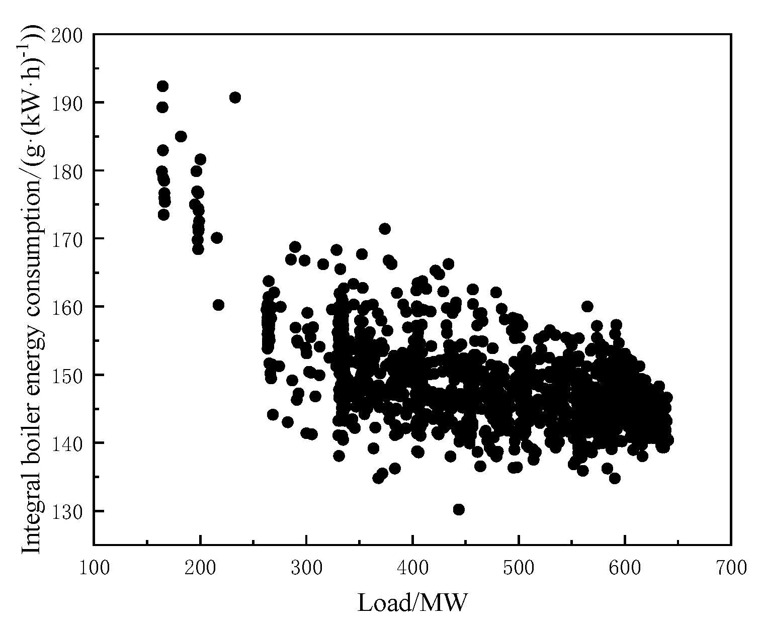
4.1.2. Calculating the Energy Consumption of the Boiler System

According to the theory of fuel specific consumption [35,36], assuming that the output power of the unit is P and the amount of fuel consumed is B, exergy is embodied in $e_p$ and $e_f$, respectively, and the sum of irreversible loss of chemical energy to electrical energy is ${\displaystyle \sum I_i}$, we can obtain:

$$B{e}_f=P{e}_p+{\displaystyle \sum I_i}$$

(15)

Divide the left and right by $P\cdot e_f$ to obtain the unit consumption analysis model of power generation:

$$b=b_{\min }+{\displaystyle \sum b_i}$$

(16)

where $b=B/P$ is the actual power consumption of the unit; $e_p$ is the exergy of electrical energy of 1 kW·h/(kW·h); $e_f$ is the exergy of standard coal of 7000 Kcal, and $b_{\min }=e_p/e_f$ is the theoretical power generation unit consumption of 123 g/(kW·h). This means that without any energy loss, 123 g of standard coal can produce 1 kW·h of electricity; $b_i=I_i/\left(P·e_f\right)$ is the additional energy consumption of the unit corresponding to the irreversible loss of the i-th link or equipment.

Using the above theory, we calculated the irreversible loss of each piece of boiler equipment, such as the economizer, water wall, low temperature superheater, platen superheater, final superheater, low temperature reheater, final reheater, and air preheater. Then, we calculated the energy consumption of each piece of equipment and summed them up to obtain the integral boiler energy consumption. Some of the calculation results are shown in

Table 4. Energy consumption of boiler system equipment.

Time	Economizer /(g·(kW·h)−1)	Water Wall /(g·(kW·h)−1)	Low Temperature Superheater /(g·(kW·h)−1)	Platen Superheater /(g·(kW·h)−1)	…	Integral Boiler System /(g·(kW·h)−1)
01/07/2022 00:00:00	7.367	60.757	19.311	8.059	…	152.218
01/07/2022 00:05:00	7.420	60.980	19.211	7.949	…	152.463
01/07/2022 00:10:00	7.500	61.840	19.136	7.791	…	152.946
01/07/2022 00:15:00	7.487	61.817	19.274	7.615	…	152.883
01/07/2022 00:20:00	7.499	61.782	19.293	7.478	…	152.732
…	…	…	…	…	…	…
01/08/2022 00:00:00	7.164	60.084	19.708	9.086		149.170

Using the water wall as an example, the calculation results include both the irreversible loss of heat transfer and the irreversible loss of chemical energy from coal converted into heat energy.

.

Figure 4 presents a schematic diagram of the energy consumption of the boiler system at different loads. The average energy consumption of the unit, based on 872 sample points with over 95% load, was approximately 142.72 g/(kW·h). When the load was below 40%, the energy consumption began to rise significantly. The load dropped below 30% for 44 sample points, and the average energy consumption was about 178.28 g/(kW·h), which was an increase of 29.56 g/(kW·h) compared to 95% load or above, representing an increase of about 20.7%.

Additionally, 141 sample points within the load range of 626–628 were selected, that is, the unit was operating close to 95% load. The boiler system’s minimum energy consumption within the range was then statistically obtained to be 140.21 g/(kW·h), while the maximum was 149.86 g/(kW·h), resulting in a difference of 9.65 g/(kW·h). These results indicate a significant variation in energy consumption for the target unit’s boiler system, highlighting a considerable potential for energy savings.

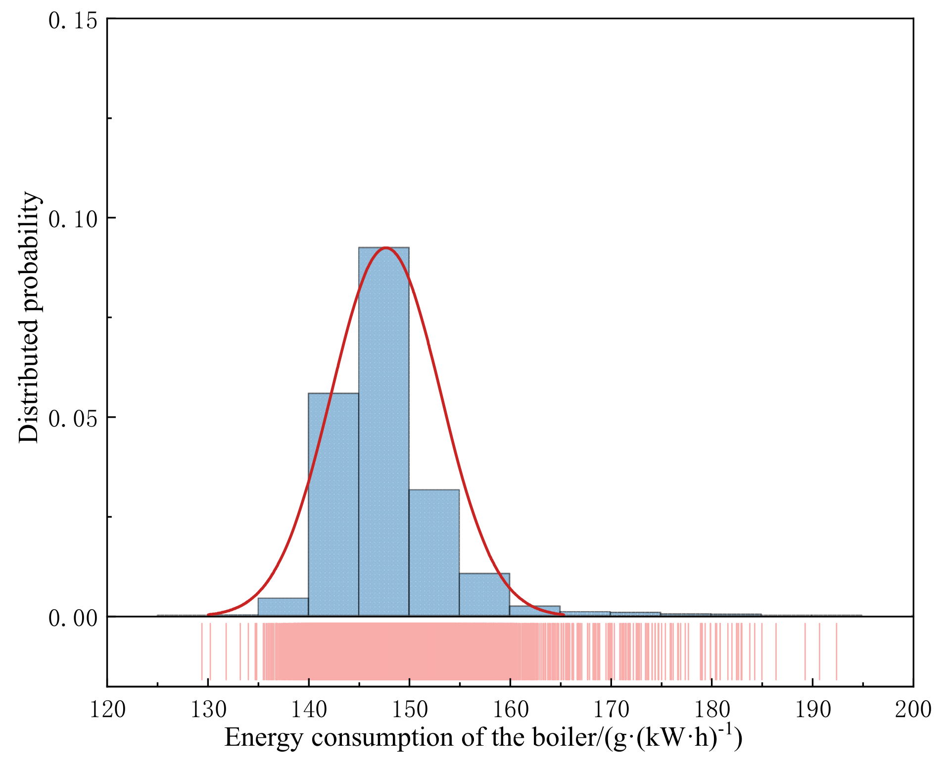
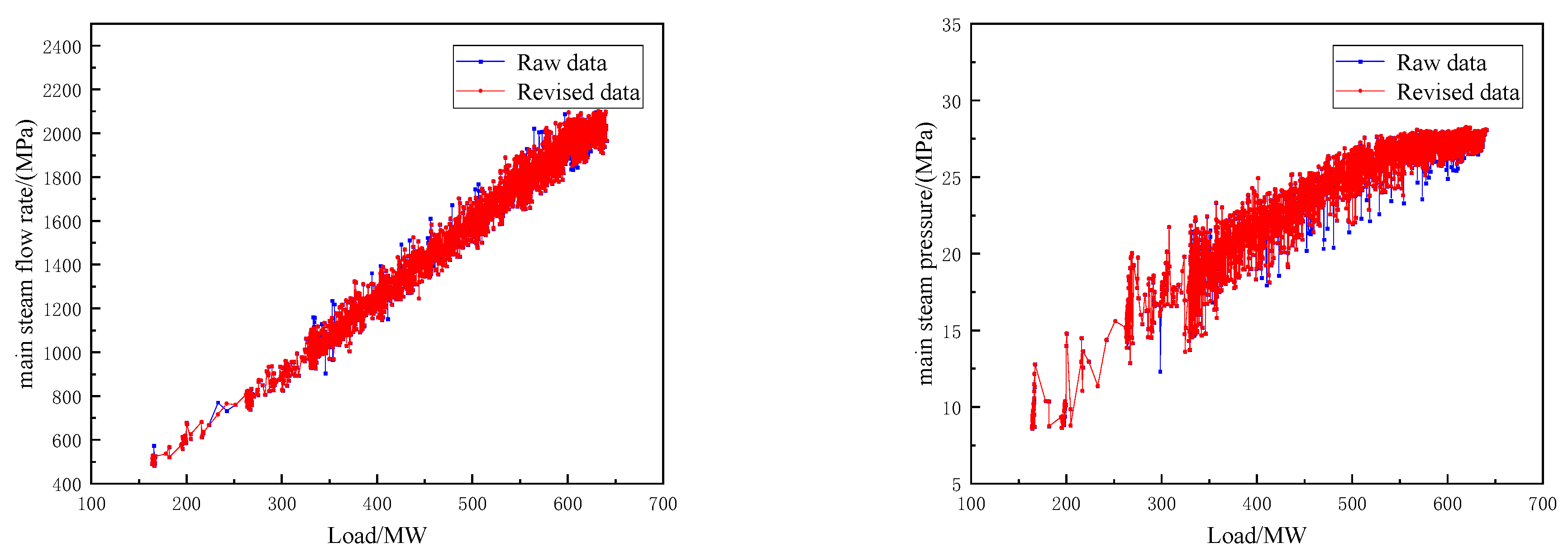
4.1.3. Removing Outliers

The accuracy of the measuring instrument and means affects the unit’s data, leading to potential errors. These errors can increase model inaccuracies and weaken the effectiveness of data mining. Therefore, it is crucial to clean abnormal data before establishing an energy consumption prediction model. For instance, it was discovered that the coal feed measurement point of a coal mill was not 0 when the mill was shut down, but instead of being a small value. To rectify such clearly erroneous data, it was artificially modified to 0. In addition, using the unit operating at 606–607 MW as an example, there are 730 samples in this range. Figure 5 shows the distribution of energy consumption of the boiler system under this condition. It was discovered that the energy consumption of the boiler system differed due to the difference in its operating state and regulation mode, despite having a similar unit operating load. However, it can be assumed that the energy consumption of the boiler system follows a normal distribution under the same working conditions, with particularly high or low energy consumption being rare cases.

Based on the analyses above, the 3-sigma criterion was selected for outlier detection in this paper. First, the dataset was arranged in descending order according to the load order, and the interval was divided into intervals of 50 samples; then, the mean e and standard deviation μ of each interval were calculated, and the samples that were not in the range (e − 3μ, e + 3μ) were recorded as outliers; finally, to ensure continuity and coherence of the dataset, the Lagrange interpolation method was used to calculate a new value based on the two samples preceding and following the outlier. The outlier was then replaced with this new value. Taking the main steam flow rate and main steam pressure as an example, their distribution with unit load before and after data processing is shown in Figure 6. It can be seen that after clearing outliers, the distribution of data was more stable and concentrated, which is more in line with the actual trend.

4.2. Feature Selection

4.2.1. Data Standardization

There are various types of measurement data for thermal power units, such as pressure, temperature, flow rate, and other parameters. To eliminate the influence of different data dimensions and numerical sizes before establishing the prediction model, this paper used extreme value standardization to process the dataset. The formula for this process is given below:

$${x_{ij}}^{\prime }=\frac{x_{ij}-x_j^{\min }}{x_j^{\max }-x_j^{\min }}$$

(17)

where: ${x_{ij}}^{\prime }$ is the standardized data; $x_{ij}$ is the j-th characteristic variable value of the i-th sample data; $x_{ij}^{\min }$ is the minimum value of the j-th characteristic variable; $x_{ij}^{\max }$ is the maximum value of the j-th characteristic variable.

4.2.2. Feature Selection Result

The MIV algorithm can be used to obtain the MIV value of each input feature for each output. However, since this paper studies a multi-input and multi-output prediction model, the MIV value of each feature for all outputs can be summed to obtain the MIV value of the feature for the entire output. To ensure the objectivity of the research results, 10-fold cross-validation was used for calculation, and the results were averaged.

As shown in

Table 5. MIV values for each feature.

Features	Absolute Value of MIV	Sum of Current Feature’s MIV	Percentage
main steam flow rate	1.4531	1.4531	0.1209
steam pressure at the outlet of final reheater	0.8112	2.2643	0.1884
feed water flow rate	0.7240	2.9883	0.2487
main steam pressure	0.5148	3.5031	0.2916
feed water temperature	0.4650	3.9681	0.3303
…	…	…	…
flame intensity of furnace D	0.0002	12.0154	1.0000

, after taking the absolute value of MIV for each feature, they were arranged in order of size. We were able to obtain the percentage of “sum of current feature’s MIV” in “sum of all features’ MIV”, that is, the correlation degree of all variables from the first feature to the current feature with the model output. In order to ensure the model was more accurate, a threshold of 90% was selected, and the number of features in the filtered dataset was reduced by 50% from 166 to 74.

There is a strong correlation between the features of a coal-fired unit. To simplify the dataset, we used Spearman correlation to screen 74 features obtained for the second time. The threshold was set at 0.95, and redundant features were removed, resulting in a final dataset of 26 features, and the features of the processed dataset are shown in

Table 6. Model input features after filtering.

Number	Feature	Number	Feature	Number	Feature
1	main steam flow rate	10	steam temperature at the outlet of platen superheater	19	flue gas temperature at the outlet of air preheater
2	main steam pressure	11	oil supply master pipe flow rate	20	integrated temperature of cold end of air preheater
3	steam temperature at the outlet of low temperature superheater	12	water pressure at the inlet of low temperature economizer	21	coal–water ratio
4	steam temperature at the outlet of separator	13	the outlet air temperature at the outlet of secondary air heater	22	separator wall temperature
5	steam temperature at the inlet of final superheater	14	steam temperature at the outlet of final reheater	23	SO2 concentration at the inlet of chimney
6	total boiler air volume	15	steam temperature at the inlet of final reheater	24	wind pressure at the outlet of mill
7	steam temperature at the outlet of final superheater	16	temperature of primary air at the outlet of air preheater	25	flue gas temperature at the outlet of low temperature superheater
8	intermediate superheating	17	the temperature of the steam before the reheater desuperheater	26	flue gas temperature at the inlet of low temperature superheater
9	water temperature at the outlet of condenser	18	steam temperature at the inlet of low temperature reheater

.

4.3. Model Prediction Results

The multi-objective prediction model MIV-ISAO-LSSVM was established by randomly dividing the training and test sets in an 8:2 ratio. In addition to the aRRMSE mentioned earlier, Mean Absolute Error (MAE) was also used to evaluate the model’s performance for each output [33], which represents the average absolute error between the predicted and true values of the test set. The formula for calculating MAE is as follows:

$$MAE=\frac{1}{N}{\displaystyle \sum _{i=1}^N\left|y_i^{\left(j\right)}-{\widehat{y}}_i^{\left(j\right)}\right|}$$

(18)

where N represents the number of samples. The variable $y_i^{\left(j\right)}$ represents the actual value of target j corresponding to test set sample i, while ${\widehat{y}}_i^{\left(j\right)}$ represents the predicted value of target j corresponding to sample i of the test set.

To verify the effect of the LSSVM prediction model optimized by the ISAO algorithm, we established LSSVM, BP, and ELM prediction models based on the same training and test sets. For LSSVM, we set the hyperparameters σ and γ to 30 and 50, respectively, while BP and ELM had a hidden layer containing seven nodes. We also used optimization algorithms such as PSO, SSA, and WOA to optimize the LSSVM model. The three algorithms and the ISAO algorithm were set to T = 50 and N = 20.

Table 7. Evaluation results of different algorithms.

Evaluation Index		ISAO-LSSVM	LSSVM	BP	ELM	PSO-LSSVM	SSA-LSSVM	WOA-LSSVM
aRRMSE		0.2747	0.2807	0.3355	0.4605	0.2747	0.2747	0.2747
MAE	integral boiler	1.0690	1.0811	1.3469	1.6693	1.0689	1.0689	1.0689
	economizer	0.1435	0.1516	0.2177	0.2231	0.1435	0.1435	0.1435
	water wall	0.6044	0.6105	0.8596	1.1897	0.6044	0.6044	0.6044
	low temperature superheater	0.2072	0.2029	0.2578	0.5851	0.2072	0.2072	0.2072
	platen superheater	0.1319	0.1335	0.1413	0.2895	0.1319	0.1319	0.1319
	final superheater	0.0778	0.0821	0.0988	0.1604	0.0778	0.0778	0.0778
	low temperature reheater	0.1169	0.1203	0.1433	0.2060	0.1169	0.1169	0.1169
	final reheater	0.0747	0.0752	0.1418	0.1475	0.0747	0.0747	0.0747
	air preheater	0.1772	0.1737	0.2108	0.2892	0.1772	0.1772	0.1772
The number of iterations where the optimal value is found		6	/	/	/	20	14	19

shows the evaluation results of the prediction models. The aRRMSE of the ISAO-LSSVM model have reduced by 2.13%, 18.12%, and 40.3% compared to the LSSVM, BP, and ELM prediction models, respectively. This suggests that an optimization algorithm can be more effective in determining hyperparameters that align with the actual conditions of the research unit, resulting in better prediction model results than artificially set hyperparameters. Upon comparing the LSSVM prediction model before and after optimization, it was discovered that the optimized model had a higher MAE value in the index of air preheater energy consumption. This indicates a larger deviation in its prediction of air preheater energy consumption. This is due to the optimization algorithm’s aim of improving the model’s overall performance, rather than focusing on a single output index.

The LSSVM prediction model optimized by the four algorithms had the same performance in the evaluation index. The model hyperparameters determined by different optimization algorithms are basically the same; the values of σ and γ determined by ISAO, PSO, SSA, and WOA are 37.7441 and 13.1996, 37.8332 and 13.2014, 37.7441 and 13.1996, and 37.7347 and 13.1998, respectively. Based on the research problem presented in this paper, it has been found that the choice of optimization algorithm has minimal impact on the effectiveness of the prediction model. However, the ISAO algorithm requires the least number of iterations to find the optimal value, which can effectively reduce computing costs.

5. Conclusions

This paper proposes a boiler system energy consumption prediction model based on the LSSVM algorithm to help analyze the change in energy consumption of ultra-supercritical coal-fired units in the Xinjiang region under flexible peaking demand. The SAO algorithm has been improved to enhance the prediction ability of the original LSSVM algorithm. Additionally, the MIV algorithm has been introduced to optimize the model input and ensure comprehensive input information. This results in accurate prediction of the boiler system’s energy consumption. The improved algorithm and model have been verified using historical operation data from the target unit.

(1)

Using the single consumption analysis method, we calculated and analyzed the energy consumption distribution of the boiler system in the target unit based on field measurement data under variable load conditions. The results indicate that when the load of the target unit is reduced to less than 30%, the energy consumption of the boiler system increases by approximately 20.7% compared to its consumption under 95% load operation.

(2)

Compared to other optimization algorithms, the strategy proposed in this study improves the convergence speed of the ISAO algorithm. Although the performances of LSSVM prediction models obtained by different optimization algorithms are similar, the ISAO algorithm can efficiently and accurately obtain the hyperparameters of LSSVM for boiler system energy consumption.

(3)

A MIV-ISAO-LSSVM model was developed to predict the energy consumption of ultra-supercritical coal-fired boilers under various load conditions. The MIV algorithm reduces the number of dataset features from 166 to 26. This greatly simplifies the model and identifies the main factors that affect the energy consumption of the boiler system. The hyperparameters of the LSSVM model are obtained through the ISAO optimization algorithm. The model demonstrated superior accuracy, reliability, and applicability compared to other models.

The approach to modelling in this paper can be applied to other boilers, but it should be noted that different boilers have different structures or equipment, so the inputs and outputs of the model will be different from those in this paper. The historical data used to train the model for predicting boiler system energy consumption should cover the entire range of working conditions as much as possible. The number of samples should also be maximized to improve the accuracy and applicability of the model across all working conditions. In the future, we aim to integrate the prediction model presented in this paper with boiler control to offer parameter guidance for optimizing boiler operation and achieving low-energy operation without compromising the boiler’s normal output.

References

1. Siksnelyte-Butkiene, I.; Zavadskas, E.K.; Streimikiene, D. Multi-criteria decision-making (MCDM) for the assessment of renewable energy technologies in a household: A review. Energies 2020, 13, 1164. [Google Scholar] [CrossRef]
2. Ordu, M.; Der, O. Polymeric materials selection for flexible pulsating heat pipe manufacturing using a comparative hybrid MCDM approach. Polymers 2023, 15, 2933. [Google Scholar] [CrossRef] [PubMed]
3. Yang, H.; Zhuo, D.Y.; Cao, J.; Dong, Y.S.; Si, F.Q. Dynamic soft sensing modeling of NOx concentration at outlet of SCR flue gas denitration system based on DJMI-GRU. Therm. Power Gener. 2021, 50, 51–58. [Google Scholar] [CrossRef]
4. Yang, K.X.; Feng, Y.L.; Liu, M.; Yang, J. Multi-parameter Optimization and Operation Strategy of Fluegas Waste Heat and Water Co-recovery System for Coal-fired Power Plants. Proc. CSEE 2021, 41, 4566–4576. [Google Scholar] [CrossRef]
5. Sun, H.B.; Yang, J.G.; Jin, H.W.; Tu, H.; Zhou, X.; Zhao, H. NOx Prediction Model for Coal-fired Boiler Based on Bayesian Optimization-Random Forest Regression. J. Chin. Soc. Power Eng. 2023, 43, 910–916. [Google Scholar] [CrossRef]
6. Dai, B.; Wang, F.; Chang, Y. Multi-objective economic load dispatch method based on data mining technology for large coal-fired power plants. Control Eng. Pract. 2022, 121, 105018. [Google Scholar] [CrossRef]
7. Blackburn, L.D.; Tuttle, J.F.; Andersson, K.; Fry, A.; Powell, K.M. Development of novel dynamic machine learning-based optimization of a coal-fired power plant. Comput. Chem. Eng. 2022, 163, 107848. [Google Scholar] [CrossRef]
8. Wang, Z.; Yao, G.; Xue, W.; Cao, S.; Xu, S.; Peng, X. A Data-Driven Approach for the Ultra-Supercritical Boiler Combustion Optimization Considering Ambient Temperature Variation: A Case Study in China. Processes 2023, 11, 2889. [Google Scholar] [CrossRef]
9. Fu, Z.G.; Liu, B.H.; Wang, P.K.; Gao, X.W. Big Data Mining Technology Application in Energy Consumption Analysis of Coal-fired Power Plant Units. Proc. CSEE 2018, 38, 3578–3587. [Google Scholar] [CrossRef]
10. Cai, Y. Theoretical Research on Data Mining Based on Energy Saving and Consumption Diagnosis for Thermal Power Units. Master’s Thesis, Zhejiang University, Hangzhou, China, 2018. [Google Scholar]
11. Xiao, H.; Xue, Y.L.; Liu, P.; Li, Z. Optimum Exergy Efficiency Analysis of Coal-fired Power Plants Based on Operation Data. Proc. CSEE 2019, 39, 164–170. [Google Scholar] [CrossRef]
12. Sun, Y.P.; Wang, L.F.; Zhang, Z.W.; Yang, Q. Genetic optimization model of power supply coal consumption for thermal power unit based on random forest. Inf. Commun. Technol. Policy 2021, 47, 76–82. [Google Scholar] [CrossRef]
13. Wan, A.P.; Yang, J.; Miao, X. Boiler Load Forecasting of CHP Plant Based on Attention Mechanism and Deep Neural Network. J. Shanghai Jiao Tong Univ. 2023, 57, 316–325. [Google Scholar] [CrossRef]
14. Wang, Y.O.; Chen, Y.F.; Mou, K.Y.; Ren, S.J. Study on index system construction of energy consumption and economic diagnosis of thermal power unit. J. Eng. Therm. Energy Power 2022, 37, 175–185. [Google Scholar] [CrossRef]
15. Wang, W.; Wei, Y.; Teng, X. Short-Term Wind Power Forecasting Based On VMD-SSA-LSSVM. Acta Energiae Solaris Sin. 2023, 44, 204–211. [Google Scholar] [CrossRef]
16. Lan, M.W.; Li, Y.; Zhao, G.Q. Study on boiler combustion modeling based on MAPSO optimizing LSSVM model parameters. J. Cent. South Univ. Sci. Technol. 2022, 53, 1506–1515. [Google Scholar] [CrossRef]
17. Deng, L.; Liu, S. Snow ablation optimizer: A novel metaheuristic technique for numerical optimization and engineering design. Expert Syst. Appl. 2023, 225, 120069. [Google Scholar] [CrossRef]
18. Li, C.; Luo, G.; Qin, K.; Li, C. An image encryption scheme based on chaotic tent map. Nonlinear Dyn. 2017, 87, 127–133. [Google Scholar] [CrossRef]
19. Zhuo, X.H.; Feng, Y.C.; Chen, L.; Luo, W.G.; Liu, S.Y. Transformer fault diagnosis based on SVM optimized by the improved bald eagle search algorithm. Power Syst. Prot. Control 2023, 51, 118–126. [Google Scholar] [CrossRef]
20. Bai, X.; Bai, Y.G. Support vector machine and feature selection simultaneous optimization based on improved Harris hawk algorithm. Comput. Eng. Des. 2023, 44, 1537–1546. [Google Scholar] [CrossRef]
21. Abualigah, L.; Yousri, D.; Abd Elaziz, M.; Ewees, A.A.; Al-Qaness, M.A.; Gandomi, A.H. Aquila optimizer: A novel meta-heuristic optimization algorithm. Comput. Ind. Eng. 2021, 157, 107250. [Google Scholar] [CrossRef]
22. Rashedi, E.; Nezamabadi-pour, H.; Saryazdi, S. GSA: A Gravitational Search Algorithm. Inf. Sci. 2009, 179, 2232–2248. [Google Scholar] [CrossRef]
23. Hatta, N.M.; Zain, A.M.; Sallehuddin, R.; Shayfull, Z.; Yusoff, Y. Recent studies on optimisation method of Grey Wolf Optimiser (GWO): A review (2014–2017). Artif. Intell. Rev. 2019, 52, 2651–2683. [Google Scholar] [CrossRef]
24. Chen, X.; Cheng, L.; Liu, C.; Liu, Q.; Liu, J.; Mao, Y.; Murphy, J. A WOA-based optimization approach for task scheduling in cloud computing systems. IEEE Syst. J. 2020, 14, 3117–3128. [Google Scholar] [CrossRef]
25. Abdollahzadeh, B.; Gharehchopogh, F.S.; Mirjalili, S. African vultures optimization algorithm: A new nature-inspired metaheuristic algorithm for global optimization problems. Comput. Ind. Eng. 2021, 158, 107408. [Google Scholar] [CrossRef]
26. Wu, C.; Fu, J.; Huang, X.; Xu, X.; Meng, J. Lithium-Ion Battery Health State Prediction Based on VMD and DBO-SVR. Energies 2023, 16, 3993. [Google Scholar] [CrossRef]
27. Liu, D.; Liu, F.; Xu, Y.P. Short-term PV output forecast based on MIV-PSO-BPNN. Acta Energiae Solaris Sin. 2022, 43, 94. [Google Scholar] [CrossRef]
28. Sun, J.J. Prediction of Pier Scour Depth Based on GA-MIV-BP Neural Network. Master’s Thesis, Nanchang University, Nanchang, China, 2022. [Google Scholar]
29. Chen, Y.; Li, M. Evaluation of influencing factors on tea production based on random forest regression and mean impact value. Agric. Econ. Zemědělská Ekon. 2019, 65, 340–347. [Google Scholar] [CrossRef]
30. Suykens, J.A.; Vandewalle, J. Least squares support vector machine classifiers. Neural Process. Lett. 1999, 9, 293–300. [Google Scholar] [CrossRef]
31. Shi, M.; Tan, P.; Qin, L.; Huang, Z. Research on Valve Life Prediction Based on PCA-PSO-LSSVM. Processes 2023, 11, 1396. [Google Scholar] [CrossRef]
32. Xie, L.R.; Wang, B.; Bao, H.Y.; Liang, W.; Maimaitireyimu, A. Super-Short-Term Wind Power Forecasting Based On EEMD-WOA-LSSVM. Acta Energiae Solaris Sin. 2021, 43, 94. [Google Scholar] [CrossRef]
33. Borchani, H.; Varando, G.; Bielza, C.; Larranaga, P. A survey on multi-output regression. Wiley Interdiscip. Rev. Data Min. Knowl. Discov. 2015, 5, 216–233. [Google Scholar] [CrossRef]
34. He, D.B.; Sun, S.X.; Liang, X.; Xie, L.; Zhang, K. Multi-target feature selection algorithm based on adaptive graph learning. Control. Decis. 2023, 1–9. [Google Scholar] [CrossRef]
35. Song, Z.P. Consumption Rate Analysis: Theory and Practice. Proc. CSEE 1992, 1992, 17–23. [Google Scholar] [CrossRef]
36. Wang, J.; Duan, L.; Yang, J.; Yang, M.; Jing, Y.; Tian, L. Energy-Saving Optimization Study on 700 °C Double Reheat Advanced Ultra-Supercritical Coal-Fired Power Generation System. J. Therm. Sci. 2023, 32, 30–43. [Google Scholar] [CrossRef]
Figure 1. Fitness values of different algorithms. labels (af) display the fitness value iteration curves of different optimization algorithms applied to the test functions F3, F8, F13, F18, F23, and F29, respectively.
Processes 12 00422 g001aProcesses 12 00422 g001b
Figure 2. MIV schematic diagram.
Processes 12 00422 g002
Figure 3. Diagram of the ISAO-LSSVM prediction model.
Processes 12 00422 g003
Figure 4. Coal consumption change chart of the unit boiler system.
Processes 12 00422 g004
Figure 5. Probability distribution of boiler energy consumption.
Processes 12 00422 g005
Figure 6. Before and after data processing.
Processes 12 00422 g006